The Self-Regulated Winds of Long Period Variable Stars

Abstract

Numerical models of the dynamically extended atmospheres of long period variable or Mira stars have shown that their winds have a very simple, power law structure when averaged over the pulsation cycle. This structure is stable and robust despite the pulsational wave disturbances, and appears to be strongly self-regulated. Observational studies support these conclusions. The numerical models also show that dust-free winds are nearly adiabatic, with little heating or cooling. However, the classical, steady, adiabatic wind solution to the hydrodynamic equations fails to account for an extensive region of nearly constant outflow velocity. An important process or group of processes is missing from this solution. Since gas parcels moving out in the wind are periodically overrun by pulsational waves, we investigate analytic solutions which include the effects of wave pressure, heating, and the resulting entropy changes.

In the case of dust-free winds we find that only a modest amount of wave pressure is needed to derive an analytic model for a steady, constant velocity, locally adiabatic outflow. Wave pressure is represented with a term like that in the Reynolds turbulence equation for the mean velocity. The waves damp relatively quickly with radius, as a result of the work they do in driving the mean flow. Although the pressure from individual waves is modest, the waves are likely the primary agent of the self-regulation of the dust-free winds.

In dusty Miras, the numerical models show the radiation pressure on grains and the subsequent momentum transfer to the gas, play the dominant roles in driving the wind, and wave pressure is not very important. In the models of the dusty wind, the gas variables also adopt a power law dependence on radius. Heating is required at all radii to maintain this flow, and grain heating and heat transfer to the gas are significant. Both hydrodynamic and gas/grain thermal feedbacks can transform the flow towards particular self-regulated forms.

1 Introduction

The astrophysical theory of hydrodynamic winds began with the solar wind equations proposed by Parker (1958), also see (Parker, 1963). Parker’s model predicted that the pressure gradient between the sun’s outer atmosphere and the interstellar medium would drive the wind. In subsequent years Parker’s solutions to the hydrodynamic equations have proven to be a powerful tool for studying stellar winds in general. (The analogous Bondi (1952) solutions for spherical accretion problems have proven to be equally important.)

Bird (1964a, b, c) constructed shock heated models of the solar corona and wind, which can be regarded as Parker winds with an additional heating term. However, Bird’s models were not designed to capture the highly nonlinear shock dynamics of long period variable star atmospheres (henceforth LPVs). The large-amplitude, quasi-ballistic motions behind LPV shocks were not considered (see Willson & Hill 1979 and Hill & Willson 1979). Nonetheless, a number of important results relevant to Miras were anticipated, including: acoustic heating of the circumstellar gas, a dynamic balance between shock heating and expansion cooling in the wind, and self-regulation in the wind flow. Bird proposed these as driving forces for the solar wind and corona, which are now believed to be the result of magnetohydrodynamic dissipation (e.g., the review of Parker 1997). At the present time, these processes appear more relevant to the warm extended atmospheres and winds of dust-free LPVs (see the reviews of Willson et al. 1997, Willson 2000 for discussions of these structures). As will be described below, self-regulating processes are very important, but Bird’s conjecture that the self-regulation works to maintain a constant Mach number throughout the flow is not strictly correct.

Hartmann and MacGregor (Hartmann & MacGregor 1980, Hartmann & MacGregor 1982, also see MacGregor & Charbonneau 1997) proposed an application of solar corona and wind models with Alfvén wave heating and pressure to LPV winds. These processes are similar to the shock pressure and heating processes described below. The Hartmann and MacGregor models assumed an approximately hydrostatic corona, with waves viewed as a modest perturbation, in contrast to the strong shocks observed in LPVs. Specifically, these are polytropic wind models, without shock entropy generation. Both shock and Alfvén waves may play a role in LPV winds, but we believe that the strong pulsational shocks are dominant, so we will not consider magnetic effects in this paper.

Because LPVs have very large amplitude pulsations, they might be expected to provide difficulties for smooth wind solutions of the hydrodynamic equations. Indeed, the numerical models of Bowen (1988, 1990), and Bowen & Willson (1991) show that the atmospheres of pulsating Miras are highly dynamic. This is also true of all published numerical models of these and related stars, e.g., Fleischer et al. (1992), Feuchtinger et al. (1993), Höfner & Dorfi (1997), Steffen, Szczerba, & Schoenberner (1998), Winters et al. (2000), and Höfner et al. (2003). Most of these models do not include non-LTE radiative cooling, so in the remainder of this paper we will primarily refer to Bowen’s models, and the particular runs described below. See Willson et al. (1997) for a comparison of various models.)

In the numerical models, the density near the photosphere retains a roughly exponential decline, but departs from this to a power law dependence at density value that depends on the mass outflow rate. In the transition from exponential to power law decline, the dynamical lifting by shocks followed by (in some cases) radiation pressure on grains lifts and accelerates the material. In this flatter density profile, more gas has been lifted to large radii, and this along with radiation pressure on dust grains in some cases, provide the means for driving much enhanced winds. Bowen’s models show that the inner atmosphere is a complex region where shock acceleration and heating and cooling all play important roles (see Willson et al. 1997). On the other hand, the wind region at large radii has a simpler structure, and the gas variables averaged over pulsation period can be well approximated as simple power law functions of radius (see Figures 1-3 and discussion below). Such simple profile forms suggest that it should be possible to construct simple analytic models in the tradition of Parker and Bird, at least for the smooth wind region.

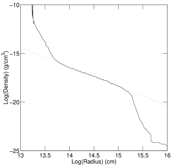
Figure 1: Density profile from a dust-free, hydrodynamical model like those of Bowen (1988). The model was run for a very long time to allow a large steady wind region to develop and relax out to $r\simeq 10^{15}cm$. (See text for details). The dotted line shows an a $\rho\propto r^{-2}$ function (normalized to the numerical model at log(r) = 14.5) for comparison.

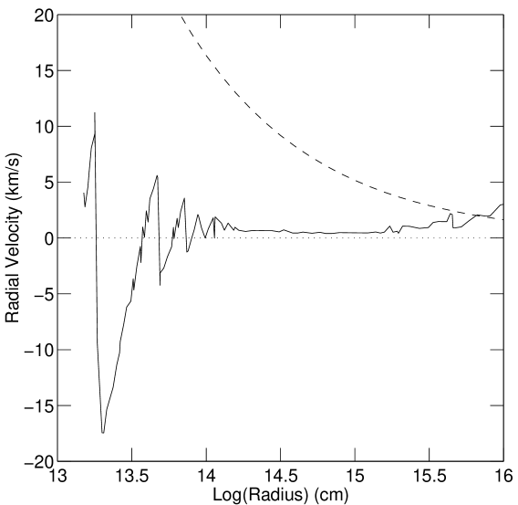
Figure 2: Radial velocity profile from the end of the same dust-free Bowen model shown in the previous figure. Comparison to the dotted line at zero velocity shows the low, constant value of the outflow in the steady wind region. The upper dashed line shows the local escape velocity. The lower dashed curve shows a fit derived from an analytic model, see Sec. 2.6 for details.

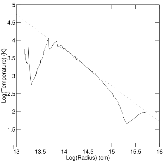
Figure 3: Temperature profile from the end of the same long, dust-free Bowen model shown in the previous figures. The dotted line shows an a $T\propto r^{-1}$ function (normalized to the numerical model at log(r) = 14.5) for comparison.

We will not consider LPV observations in detail in this paper, since our main goal is to understand the regularities revealed by numerical models. In addition, the constraints on theory provided by observation (e.g., spectra) are indirect, and generally the comparison between theory and observation is best done with the aid of detailed numerical models (see e.g., Willson 2000, Tej et al. 2003 and references therein). Nonetheless, some recent observations provide quite direct information about the gas variables in the winds and extended atmospheres of LPVs, and a brief mention of these provides a context for the subsequent work.

First of all, a major assumption of both analytic and numerical models is that the LPV winds are approximately spherically symmetric. In spite of evidence for modest deviations from symmetry, or asymmetries in binary systems, there is much evidence from a variety of wavebands for approximate symmetry in most cases (e.g., Bujarrabal & Alcolea 1991).

Recent infrared interferometric observations of “dust shells” around Miras are also generally consistent with spherically symmetric models, though not with uniform dust density distributions. The data are better fit by models including a few distinct shells where the dust emission is high (see e.g., Hale et al. 1997, Lopez et al. 1997, Monnier et al. 1997, Fong, Meixner, & Shah 2003, and references therein). However, these observations probe a region located at a distance of only a few stellar radii, where conditions are described as dynamic and complex. In fact, the numerical models show that this is the region where shocks have grown to very nonlinear amplitudes, where dust forms if it is able to, and where the wind is just beginning to be accelerated (the “shock acceleration” and “dissipation” zones of Willson et al. 1997). Thus, these observations generally support the picture provided by the models, and do not contradict the notion of a generally smooth wind structure.

Observations and models are in general agreement about basic wind parameters like the mass loss rate or flow velocity. From CO observations (e.g., Bujarrabal & Alcolea 1991, Kahane & Jura 1994, Young 1995, Kerschbaum & Olofsson 1998, Groenewegen et al. 1999, and Winters et al. 2002, also see Alard et al. 2001 for mid-infrared results) we know that mass loss rates range from $10^{-7}M_{\odot}/yr$ up to $10^{-5}M_{\odot}/yr$ for Miras in agreement with Bowen’s models (Bowen 1988, Bowen & Willson 1991, & Willson 2000). Above about $10^{-5}M_{\odot}/yr$ the stars are generally classified as OH-IR sources. In this paper we are most interested in low mass loss rates, in relatively dust-free cases.

The dust free models develop an approximately constant outflow velocity with a speed well below the escape speed, and this pattern persists over many stellar radii. In this region the flow is also subsonic. Thus, this constant velocity is not the same as the coasting flow in standard wind models well beyond the sonic point. The observations also find low wind velocities (of order 5-10 km/s) and little evidence for changes in the flow velocity through the wind. For the Miras CO observations are able to probe the flow at large distances from the star, and so, provide important constraints on any model. Interestingly, Cepheid wind velocities also seem to be low relative to the escape speed (Sasselov & Lester 1994a, b).

In the following sections we will derive analytic wind models, described by hydrodynamic equations which including approximate, averaged terms, like those in the Reynolds turbulence equations, to represent the effects of nonlinear pulsational waves on the flow. We then discuss the self-regulatory feedbacks in these winds, and use several approaches to argue that these processes select constant velocity outflows over other possible wind solutions.

2 Wave Pressure in Dust Free Winds

2.1 Classical Steady Wind Solutions Compared to a Numerical Model

The usual Parker wind equations are derived from the steady, spherically symmetric hydrodynamic continuity and momentum equations, which can be written as,

$$\dot{M}=4\pi r^{2}\rho u$$ (1)

$$u\frac{du}{dr}=-\frac{1}{\rho}\frac{dP}{dr}-\frac{GM}{r^{2}}.$$ (2)

where the variables, $\dot{M}$, $M$, $\rho$, $P$, $u$, and $r$ denote the mass loss rate, total mass of the star, the density, pressure, wind speed, and the distance from the center of the star, respectively. Classical steady wind solutions also assume a polytropic equation of state, $P=K\rho^{\gamma}$, with constant K, $\gamma$. In this paper we will assume a constant rate of mass loss as well.

Two properties of the outer region of the atmosphere suggest that it can be described as approximately locally adiabatic: 1) the temperatures there are in a range where radiative cooling is inefficient, and 2) the shocks in this region are relatively weak. The latter feature is evident in Figures 1-3, which show density, velocity, and temperature profiles taken from the end of a very long run (about 1000 pulsation cycles) of Bowen’s modeling code, without dust.

Detailed descriptions of the atmospheric dynamics can be found in Bowen (1988). Here we merely note that the code numerically solves the one-dimensional, spherically symmetric, hydrodynamic equations with a Richtmyer & Morton (1967) type Lagrangian method, including a conventional artificial viscosity algorithm for stabilizing strong shocks. A number of different chemical rate, momentum and energy sources are calculated explicitly for each gas element. These include: the atomic radiative cooling rates, the free electron abundance, energy changes due to ionization and recombination. They also include simple approximations to the radiative transfer, grain formation, radiation pressure on grains, and grain heating and cooling. The effects of most of these processes will not be considered in this paper, which focusses instead on understanding the global hydrodynamics. However, the numerical models provide a standard for comparison, as well as assurance that the analytic models are not unrealistic. The parameters of the numerical model shown in Figures 1-3 are essentially the same as those of a dust-free, $1.0M_{\odot}$, “standard” model of Bowen (1988), though the model shown here was computed with increased spatial resolution. The numerical models will be compared to analytic models below, especially in Section 2.6.

The wind density profile shown in Figure 1 has an approximately $1/r^{2}$ form, while the form of the corresponding temperature profile is nearly $1/r$ (Fig. 3). Note that beyond a radius of $10^{15}cm$ in the figures the model wind flow is not fully relaxed. (Indeed, Fig. 3 suggests that the flow is not thermally relaxed beyond $log(r)=14.5$.) There is, in fact, a polytropic solution to equations (1) and (2), with a $1/r^{2}$ density profile, and a $1/r$ temperature profile. However, the value of the polytropic index in this model is $\gamma=3/2$. Not only does this not correspond to the adiabatic value of $\gamma=5/3$ expected in the absence of cooling and heating, it does not have any obvious physical meaning.

We should note, however, that Parker argued against values of $\gamma>3/2$ on the grounds that larger values did not yield “a solution beginning at low velocity close to the sun and extending outward to zero pressures at infinity” (Parker 1963, pg. 61). He also noted the need for a heating source when $\gamma<3/2$.

What about the adiabatic, $\gamma=5/3$ wind solution? To illustrate the problems with this classical solution we integrate equation (2) from an inner radius $r_{1}$ to an arbitrary outer radius r, use the ideal gas law and employ the definition of the adiabatic sound speed to derive the following Bernoulli equation,

$$\frac{1}{2}\biggl{(}u^{2}-{u_{1}}^{2}\biggr{)}=\frac{-1}{\gamma-1}\biggl{(}c^{2}-{c_{1}}^{2}\biggr{)}+\frac{1}{2}\biggl{(}{v_{e}}^{2}-{v_{e1}}^{2}\biggr{)}.$$ (3)

The numerical models show that the sound speed c decreases with radius approximately as $r^{-1/2}$, as does the escape velocity $v_{e}$. Thus, according to the equation (3), the flow velocity u must decrease with radius by comparable amounts. It does not; Bowen’s models show constant velocity in the wind at all times (see Fig. 2).

We note also that, if all the wind flow lies on a single adiabat in the thermodynamic phase space, and has a $1/r^{2}$ density profile, then the ideal gas law implies that the temperature goes as $T\propto r^{-4/3}$. With the long run we have performed, which yields a large wind region, the numerical profile does appear shallower than an adiabatic one.

Maintaining a shallower temperature profile requires extra heating and momentum sources in the wind. In fact, a likely reason for discrepancies between numerical models and the adiabatic solution is that, although the pulsational shocks are weak in the wind region, their momentum, heat, and entropy inputs are not negligible.

2.2 Not Quite Adiabatic Solutions with Wave Pressure and Heating

2.2.1 Wave Pressure

The question is how to capture the effects of waves in a relatively simple analytic description of the overall wind flow, averaged over many pulsation cycles? The problem is like that of describing turbulent flows in which large fluctuations on many scales coexist with a mean flow and long-lived coherent structures. The characteristics of the regular, pulsational shocks, which propagate outward through the wind, are very different from the stochastic, fluctuations described in the theory of well-developed, homogeneous turbulence (e.g., Tennekes & Lumley 1972, McComb 1990). Nonetheless, in both cases we are dealing with disturbances on small spatial scales and short timescales, which we don’t necessarily need to resolve in order to describe their average effect on the flow.

In fact, the fundamental idea of turbulence theory, that the flow can be divided into a mean and a fluctuating part, provides a very appropriate approach to generalizing the classical stellar wind equations. We cannot simply adopt the averaging procedures used to derive the Reynolds equations of turbulence theory, since these depend on the random nature of the fluctuations in homogeneous turbulence. We can, however, provide physical justifications for including similar ’averaged’ fluctuation terms in a set of phenomenological Reynolds equations for mean wind flows.

The numerical models show that each pulsational shock provides a compression and an outward boost to an individual gas element, and the gas element follows a quasi-ballistic free-fall trajectory behind the shock (Willson & Hill 1979, Hill & Willson 1979, Bowen 1988, and the review of Willson et al. 1997). More precisely, for a periodic pattern of motion in the atmosphere, the material at larger r must have smaller outward postshock speeds. This picture is good deep in the atmosphere. If the postshock speed is slightly too high, the mass element encounters the next shock at slightly larger than it did the last one. This gives a small net outward motion, as is seen in the atmosphere around 1.5-2.5 stellar radii. Where the flow dominates, the material still responds nearly ballistically, setting up a stable pattern relative to the mean flow speed and providing a small increment of momentum to the gas in each cycle. This allows us to separate the mean flow from the oscillations, which average approximately to zero (see Appendix A for details).

To incorporate the effects of the shocks on the mean flow, an additional term is included in the (inviscid) momentum equation. With the approximation of the previous paragraph, this term can be written as the divergence of a Reynolds stress, which in the spherically symmetric case is just the radial derivative of the mean square velocity fluctuation, or ${\partial}(\sigma^{2})/{\partial}r$. Physically, this is the (one-dimensional) wave pressure gradient. In the Bernoulli equation (3) it contributes a $\sigma^{2}$ term, like the sound speed term.

2.2.2 Shock Heating

The net effect of shock heating can be included as a term in the mean, steady state energy equation (see Appendix A), which can be written as,

$$\frac{1}{2}r^{-2}\frac{\partial}{\partial r}\biggl{(}r^{2}\rho u^{3}\biggr{)} = -r^{-2}\frac{\partial}{\partial r}\biggl{(}r^{2}\rho u\epsilon\biggr{)}+r^{-2}\frac{\partial}{\partial r}\biggl{(}r^{2}uP\biggr{)}$$ (4)

$$-\frac{GM\rho u}{r{2}}+\Gamma\rho.$$

The variables, $\epsilon$ and $\Gamma$ denote the internal energy per unit gas mass, and the shock heating function, respectively. Henceforth, we define u as the sum of the mean ($U=<u>$) and fluctuating ($\sigma=(u-U)$) velocity components. In turbulence theory, we assume that this is an ensemble average over many nearly identical systems, distinguished by the details of their random fluctuations. In the present case the average is also assumed to be over all pulsational phases. Similarly, $\rho,\epsilon,$ and P generally have both mean and fluctuating parts, but we will not need to adopt special symbols for the separate parts (except in Appendix A).

We re-emphasize that in this equation we neglect the effects of the interaction between wind material and the stellar radiation, the interaction with the radiation generated in different parts of the winds, and energy exchanges between gas and dust grains.

The Reynolds formalism provides an additional equation for the mean square fluctuating velocity (see McComb, sec. 1.3.2). In the case of a steady, inviscid, constant mean velocity radial flow, this equation can be written,

$$U\frac{\partial}{\partial r}\biggl{(}\sigma^{2}\biggr{)} = -\frac{\partial}{\partial r}\Biggl{[}<(u-U)^{3}>+\frac{2}{\rho}<(u-U)P>\Biggr{]}$$ (5)

$$-2{\sigma}^{2}\frac{\partial U}{\partial r}-2\Gamma.$$

The first two terms on the right-hand-side represent turbulent (or wave) energy diffusion by nonlinear couplings, which we expect to fall off quickly with radius in this case, and so will neglect them. (This neglect is part of a closure approximation for the Reynolds moment equation set.) What remains is a relation between the local wave pressure gradient and the shock heating,

$$\Gamma=-\frac{1}{2}U\frac{\partial}{\partial r}\Bigl{(}\sigma^{2}\Bigr{)}+{\sigma^{2}}\frac{\partial U}{\partial r},$$ (6)

(where the last term is small in winds with nearly constant mean velocity).

Although we now have the required energy and momentum source terms and a relation between them, the equation set is not quite complete.

2.2.3 Equation of State

We employ a locally, but not globally, adiabatic equation of state to describe the effects of shock heating in the outer atmosphere. Physically, in each pulsation cycle, any parcel of gas goes through an irreversible (non-closed) cycle in a p-V (pressure - specific volume) phase diagram. A pulsational shock wave pushes a gas parcel along a Hugoniot curve in the phase diagram, and off its initial adiabat (e.g.,Landau & Lifshitz 1959). Radiative cooling at constant pressure behind the shock then moves it to lower specific volume (i.e., compresses it). Downstream from the shock the parcel evolves along a new adiabat to higher specific volumes and lower pressures in the rarefaction region, until it is hit by the next shock. A possible laboratory analogue of this physics is provided by the reverberating shock cavities produced in the (gun-type) experiments (see Holmes et al. 1995).

For weak shocks the specific entropy changes are not great, but they accumulate. Gas parcels farther out in the wind have experienced more of these cycles, and so, lie on adiabats that are farther from the initial one than those in the inner wind. We assume that the specific entropy of the mean flow is time-independent and a smooth function of radius, like the other gas variables. We believe this gradual entropy change is an important factor in making the wind region of Bowen’s dust-free Mira models appear quite adiabatic, but with a constant outflow velocity, which is not characteristic of a classical adiabatic wind.

We can write the locally adiabatic equation of state as,

$$P=K(r)\rho^{\gamma},$$ (7)

where $\gamma=5/3$. Because gas parcels at different radii are on different adiabats, K is a function of the radius, rather than a constant. (Klahr & Bodenheimer (2003) have also recently considered model Keplerian disks with entropy gradients due to local heating.)

Since the gas is locally adiabatic, the perfect gas relationship for $\epsilon$ is valid (locally) at any radius,

$$\epsilon=\frac{P}{\rho}\frac{1}{\gamma-1}.$$ (8)

This relation completes the equation set. We have introduced three new terms into the Parker wind equations, which describe wave pressure, shock heating, and shock entropy production. None of these extra phenomenological terms are found in the gas equations that are the basis of published numerical models (e.g., Bowen 1988). Those models follow the time-dependent pulsation and shock phenomena explicitly. We believe all of the phenomenological terms are necessary to describe the locally adiabatic mean flow in pulsationally driven winds.

We note that the classical, linear treatment of waves propagating into a stellar atmosphere indicates that long period waves should be reflected at the surface. Pijpers and collaborators, described the effects of stochastic acoustic waves in detail in a series of papers (Pijpers & Hearn 1989a, Pijpers & Hearn 1989b, Koninx & Pijpers 1993, Pijpers 1993, and Pijpers 1995). They found that such waves can propagate in the context of a general outflow (see Pijpers 1993). Bowen (1990) found that the power needed to maintain large amplitude photospheric oscillations is actually lower for long periods, and these induce nonlinear wave propagation (shocks) traveling out through the atmosphere. Here we take the existence of transmitted waves as a given, and focus on the large-scale, nonadiabatic effects of mildly nonlinear waves in the wind region only.

2.3 Constant Velocity Winds and Entropy Production

Motivated by the observations, we begin by considering the simple case in which the mean wind velocity is constant, $U=U_{0}$. In this case, equation (1) immediately gives $\rho$, and the mean flow momentum (eq. (2)) can be written,

$$-\frac{1}{\rho}\frac{dP}{dr}-\frac{GM}{r^{2}}-\frac{d}{dr}(\sigma^{2})=0,$$ (9)

where $\rho$ and P are now the Reynolds average quantities.

With the additional assumption that all three terms on the left-hand-side of this equation scale the same way with radius throughout the wind flow, we can readily obtain a solution to this and the energy equation. This assumption appears quite strong, but is physically reasonable for the following reason. The wind extends over a very large range of radii. The gas thermal energy and temperature do not fall off as rapidly with radius in dust-free models as expected in an adiabatic flow. This suggests a heat source operates throughout; shock heating is the only available source. (We note that photo-heating of grains will have a similar scaling with radius, but we assuming negligible grain populations for the present.) This fact ties the thermal pressure to the shocks and suggests that it scales like the wave pressure.

Beyond this physical argument, we can briefly note the mathematical possibilities. First is the possibility that thermal pressure dominates in part of the wind and wave pressure elsewhere. In the former region we will have a Parker thermal wind, with the observational difficulties mentioned above. In the wave dominated region, we will get the same scaling with radius, which derives from balancing the gravitational term. Since shock compression does provide thermal heating, this limit isn’t physically self-consistent. A second possibility is that the thermal and wave pressures have different functional forms whose sum contrives to balance the gravitational term. For example, they could both have the same power law form derived below, but modulated by oscillatory parts which have the same amplitude for both, but which are $180^{\circ}$ out of phase. Any other solution of this type would have to be similarly fine-tuned. Given that the wind extends over orders of magnitude in radial extent, this seems physically contrived. We will argue later that the solution below is also preferred by self-regulatory processes.

Specifically, we assume that $\sigma^{2}=A/r$ for some constant A, then equation (9) becomes,

$$dP=-\Bigl{(}GM-A\Bigr{)}\frac{\rho}{r^{2}}dr.$$

Now $\rho$ can be substituted from the continuity equation and the result can be integrated (from a radius r to $\infty$) to get

$$P=\frac{1}{3}\frac{(GM-A)}{r}\rho,$$ (10)

assuming $\rho$ and P go to zero at infinite radius. It is interesting that this equation has the form $P\propto\rho^{3/2}$ of a constant velocity Parker wind, since $\frac{1}{r}\propto\rho^{\frac{1}{2}}$, though we here view the solution as only locally adiabatic, rather than globally barotropic.

Next, we want to simplify the energy equation (4) in this constant velocity case. We need the following result in taking the mean of the term on the left-hand-side of equation (4),

$$\Bigl{<}\rho{u^{3}}\Bigr{>}=\Bigl{<}\rho\Bigr{>}\Bigl{<}{U^{3}}+3{\sigma^{2}}U\Bigr{>}$$ (11)

where $\rho$ is used here as the total density (mean plus fluctuating parts). This equation assumes that the mean of odd powers of the fluctuating velocity vanish, and that the correlation $<\rho(u-U)>$ is negligible (see Appendix A). Henceforth, we drop the brackets $<>$, and assume again that $\rho$ and P refer to the mean quantities.

When we use this result, pull $U_{0}$ factors out of partial derivatives, and substitute for $\epsilon$ from equation (8), the energy equation becomes,

$$\frac{3}{2}\Biggl{(}\frac{\rho U_{0}}{r^{2}}\Biggr{)}\frac{\partial}{\partial r}\Bigl{(}{r^{2}}{\sigma^{2}}\Bigr{)}+\frac{3}{2}\Bigl{(}{U_{0}}{\sigma^{2}}\Bigr{)}\frac{\partial{\rho}}{\partial r} =$$

$$\Biggl{(}\frac{\gamma-{2}}{\gamma-{1}}\Biggr{)}\frac{U_{0}}{r^{2}}\frac{\partial{\Bigl{(}{r^{2}}P}\Bigr{)}}{\partial r}-\frac{GM{\rho}{U_{0}}}{r^{2}}+\Gamma\rho,$$ (12)

To further simplify we can substitute for P with equation (10), for $\Lambda$ with equation (6), use the substitution ${\sigma}^{2}=A/r$. The result reduces to,

$$A={\frac{5}{11}}GM,$$

and yields in turn,

$$\Gamma=\frac{5}{22}U_{0}\frac{GM}{r^{2}}.$$ (13)

The physical interpretation of the last equation is that the shock heating rate is doing work against the gravitational potential $GM/r$ at each radius, on a flow timescale of about $r/U_{0}$. It is reducing the effective gravity (i.e., the factor GM-A in eq. (10)), that must be overcome by flow down the thermal pressure gradient.

Combining equation (10) with equation (7) and the continuity equation gives the following expression for the variable $K$ in equation (7).

$$K(r)=\frac{2}{11}GM\Biggl{(}\frac{\dot{M}}{4\pi U_{0}}\Biggr{)}^{-\frac{2}{3}}r^{\frac{1}{3}},$$ (14)

and that equation becomes,

$$P=\frac{2}{11}GM\Biggl{(}\frac{\dot{M}}{4\pi U_{0}}\Biggr{)}^{-\frac{2}{3}}r^{\frac{1}{3}}\rho^{\gamma},$$ (15)

a generalized (position-dependent) polytropic relation.

To better appreciate why K varies with radius, recall that the entropy (per unit mass) of a perfect gas is,

$$S=log\Bigl{(}{P/\rho^{\gamma}}\Bigr{)},$$ (16)

so equation (7) implies $S=\log(K)$. Thus, K is directly related to entropy, and its radial dependence implies a mean radial entropy gradient. As any gas element flows outward, it is overtaken by shocks moving through the wind, and each shock increases the entropy of the element. At any fixed radius the entropy production is balanced by the outward transport.

The value for the constant A above implies that the wave energy is about 45% of the gravitational potential energy at all radii. This implies that $\sigma$ should be about half the value of the escape velocity at any radius. The velocity ”jitter” due to shocks in Bowen’s dust-free numerical models is considerably less than this, generally less than a third of the escape velocity.

However, it is not clear that this velocity jitter should be directly identified with $\sigma$, see section 2.6 below. We expect difficulties in capturing the full range of velocity variation in the models. Most of this variation occurs across thin shocks, and these short wavelength variations are not well resolved numerically.

2.4 Accelerating Winds

The constant velocity wind described above is an especially simple solution to the equations. In this section we consider steady accelerating winds with radially dependent mean velocities. We restrict our consideration to power law similarity solutions. Mathematically, we are essentially exploring a specific kind of variation of the previous solution, but self-similar winds are the most relevant physically.

Specifically, we assume $U=U_{0}(r/r_{0})^{\delta}$, so $\rho=\frac{\dot{M}r_{0}^{\delta}}{4\pi u_{0}}r^{-(2+\delta)}$. In this case, the mean momentum equation is,

$$U\frac{dU}{dr}=-\frac{1}{\rho}\frac{dP}{dr}-\frac{GM}{r^{2}}-\frac{d}{dr}\Bigl{(}\sigma^{2}\Bigr{)}.$$ (17)

To solve this equation we will again assume a specific form for the wave pressure term, that is,

$$\sigma^{2}=\frac{A}{r}+B\Biggl{(}\frac{r}{r_{0}}\Biggr{)}^{2\delta},$$ (18)

where the first term is as in the constant velocity case, and the second term is designed to adjust the wave pressure in accordance with the flow acceleration. Like A, the coefficient B is independent of radius, but does depend on the exponent $\delta$. Note that in the case $\delta=0$, this expression does not coincide with the previous one for constant flow unless we add an additional term of -B. This term complicates the algebra of the model considerably, and since we usually have $|B|<<A/r_{0}$ (see below), we will neglect it for the moment.

We could also add other power law terms to the expression for the wave pressure, or pursue a series solution for the wind variables. We believe this would only complicate the equations without adding much physical insight.

An expression for the pressure can now be derived by integrating the momentum equation as before. We obtain,

$$P(r) = \Biggl{(}\frac{1}{3+\delta}\Biggr{)}\Bigl{(}GM-A\Bigr{)}\frac{\rho(r)}{r}+$$ (19)

$$\Biggl{(}\frac{\delta}{\delta-2}\Biggr{)}\Biggl{(}1+\frac{2B}{U_{0}^{2}}\Biggr{)}{U_{0}^{2}}\rho(r)\Biggl{(}\frac{r}{r_{0}}\Biggr{)}^{2\delta}.$$

The function K(r) can be derived by substituting equation (7) for P.

Next we substitute equation (18) (with nonconstant U) into the ${\sigma}^{2}$ equation (5) (including the term for the flow of energy from the mean field to the fluctuating velocity field, $-2{\sigma}^{2}\frac{\partial U}{\partial r}$). This produces a rather complex expression for the heating,

$$\Gamma=\frac{U_{0}}{2r_{0}}\Biggl{[}\Bigl{(}1-2\delta\Bigr{)}\frac{A}{r_{0}}\Biggl{(}\frac{r}{r_{0}}\Biggr{)}^{\delta-2}-4\delta B\Biggl{(}\frac{r}{r_{0}}\Biggr{)}^{3\delta-1}\Biggr{]}.$$ (20)

Finally, the above expressions can be substituted into the energy equation to derive the following expressions for the coefficients A and B as functions of the exponents $\gamma$ and $\delta$ by equating the coefficients of the equal powers of $\delta$,

$$A=\frac{\Bigl{[}(2-\gamma)-(3+\delta)(\gamma-1)\Bigr{]}}{\Bigl{[}(2-\gamma)-(2-\delta)(3+\delta)(\gamma-1)\Bigr{]}}GM,$$ (21)

$$B=\frac{\Bigl{[}-(\gamma-1)(2-\delta)+(2-\gamma)2\delta\Bigr{]}}{\Bigr{[}5(\gamma-1)(2-\delta)-4\delta(2-\gamma)\Bigr{]}}{U_{0}^{2}}.$$ (22)

The equations (20)-(22) specify the net heating required to maintain the power law velocity profile. They do not directly take into account the dependence of specific heating processes, like shock heating, on the gas quantities, but rather assume that such processes can be regulated to the form above. However, the expression for the heating profile (eq. (20)) is so complex that it seems unlikely that realistic shock heating and radiative cooling processes would generate it. This is in contrast to the simple heating profile of equation (13) for the constant velocity outflow, and suggests that the simpler form would be preferred (as it is in Bowen’s numerical models). This question will be examined more carefully in the next section.

Before continuing, however, we note a couple of peculiarities of the equations above. First of all, in the limit of $|\delta|<<1$ and $\gamma=5/3$ (locally), the expressions for A and B become,

$$A=\frac{5}{11}GM\biggl{(}1+\frac{32}{55}\delta\biggr{)},$$ (23)

$$B=-\frac{1}{5}{U_{0}^{2}}\biggl{(}1-\frac{3}{10}\delta\biggr{)}.$$ (24)

B is negative, and not directly proportional to $\delta$. This means that in the accelerating wind, the wave pressure could be reduced at $r<r_{0}$ relative to the constant velocity flow. Physically, it is more reasonable to simply identify $r_{0}$ as the inner radius of the wind (see eq. (18)).

Another peculiarity is that if, as we expect, the heating is dominated by the first term in equation (20), it becomes negative when $\delta$ is increased above a value of 1/2, which implies a cooling process. This also seems unphysical.

2.5 Self-Regulation

2.5.1 General Considerations

The simple appearance of the profiles of gas variables in Bowen’s dust-free numerical models suggests that the system relaxes to a self-similar solution, independent of the details of the shock heating, and subsequent expansion cooling. We have suggested above that one key to deriving this solution is the assumption that the gas in the wind is only locally adiabatic. This assumption allows for entropy production in weak shocks, which gradually evolves a gas element through a sequence of adiabats as it moves outward in the wind.

The thermal state of the gas determines the environment traversed by the shocks, which in turn are responsible for producing this state. This feedback in the shock heating mechanism eventually works to regulate the wind to the $1/r^{2}$ density profile.

The process of self-regulation is well illustrated by the early relaxation that occurs in Bowen’s numerical models, which are started with small (but increasing) pulsation amplitudes, and with an exponential atmospheric density profile. As described in Bowen 1988 the traveling wave parts of the pulsations steepen into strong shocks as they propagate down the initial exponential atmospheric profile. These shocks launch gas parcels out on quasi-ballistic trajectories (Willson & Hill 1979 and Hill & Willson 1979) to such large radii that they are not able to fall back to their starting points before being hit by the next shock. As a result, the initial profile is stretched out into power law form. This causes a feedback, the shock acceleration is decreased in the flatter pressure profile, and the ballistic launch velocities are moderated. Thus, if the pressure profile is steeper than $1/r^{3}$, then the shock amplitude grows, pushing material out, until it matches that form (see Appendix B). If the density gradient is shallower, however, the loss of energy in pushing the gas will lead to declining shock amplitudes, and it will not be possible to hold the shallow profile up against gravity. A pressure gradient that is neither too steep, nor too flat, also maintains the flat outflow velocity.

The steady gas variable profiles that are eventually established with finite amplitude pulsations include another region between the exponential atmosphere where shocks grow nonlinearly, and the power law wind region. This is the shock dissipation region where the power law density profile flattens, but the temperature and pressure increase with radius to a maximum, forming a warm “Calorisphere” and the inner boundary of the wind. See the review of Willson et al. (1997) and references therein for more details. The development of this region in the numerical models provides a clear example of the effects of shock dissipation when density and pressure profiles flatten.

This qualitative discussion on relaxation processes, which was partially anticipated by Bird 1964c, helps us understand why there is a preferred wind profile. However, it is not yet sufficiently precise to predict the form of that profile. Next we will consider some more quantitative approaches to the problem.

2.5.2 Nonequilibrium Thermodynamics and Least Dissipation

The relaxation to the simple, constant velocity flow is driven, in part, by the tendency of such a system towards a state of least dissipation, or minimum entropy production. Such states often correspond to those of maximum entropy content. The Theorem of Minimum Entropy Production for steady, nonequilibrium states derives from work of Helmholtz, though it has been generalized and used in a variety of applications in the last few decades (see e.g., Glansdorff & Prigogine 1971, Prigogine 1980, Woods 1996). Proofs of the different versions of this theorem involve substantial restrictions, e.g., that the system is not too far from thermodynamic equilibrium, or that there are linear relations between the flow variables and their driving force or source terms (like the familiar linear stress-strain relation), see Woods (1996).

These theorems have not been used much in astrophysics, where there are many non-equilibrium systems, but where these systems are often highly time-dependent. On the other hand, the winds of long-period variables appear to provide an astrophysical situation where the theorem can be usefully applied. If pulsations begin with small amplitudes and build up steadily, then the wind can adjust to this changing driving, and never find itself too far from a set of local equilibria. Moreover, equation (9) (neglecting the last term) appears to give the linear relation required of the dissipative quantities in some proofs (see Woods 1996). The minimization of shock dissipation also seems to be in accord with the qualitative considerations of the previous subsection.

We can apply the theorem by comparing the net production of the entropy in the accelerating wind models. The theorem implies that the wind with minimal entropy production is the preferred state. In principle, we need to consider the details of the dissipational processes, which is very complex in the present case. Fortunately, it seems clear physically that the entropy production in the steady winds must be directly related to the shock heating function $\rho\Gamma$ (see eq. (20)). Thus, for the purposes of making a simple estimate, we define a function, H, as follows,

$$H=\Biggl{(}\frac{2}{\dot{M}}\Biggr{)}\int_{r_{0}}^{r_{1}}4\pi{r^{2}}\rho\Gamma dr$$ (25)

where $r_{0}$ and $r_{1}$ are adopted inner and outer bounds of the wind region. The coefficient $(2/{\dot{M}})$ is included merely to absorb that common factor from the continuity equation into the definition of H, which then has units of velocity squared. Substitution for $\rho\Gamma$ and integration yields,

$$H=\Bigl{(}1-2\delta\Bigr{)}\frac{A(\delta)}{r_{0}}\Biggl{(}1-\frac{1}{x_{1}}\Biggr{)}+2B(\delta)\Bigl{(}1-{x_{1}^{2\delta}}\Bigr{)},$$ (26)

where the functions A and B are given by equations (21) and (22) with $\gamma=5/3$, and $x_{1}={r_{1}}/{r_{0}}$. Note that the outer boundary of the wind, ${r_{1}}$, will generally be a function of $\delta$, which governs the density falloff. For example, we can make a simple estimate by assuming that the outer boundary is where the mean flow velocity U equals the escape velocity. In that case, we have,

$$x_{1}=\frac{r_{1}}{r_{0}}=\Biggl{(}\frac{2GM}{{r_{0}}{U_{0}^{2}}}\Biggr{)}^{\frac{1}{1+2\delta}}.$$ (27)

The dimensionless factor $({U_{0}^{2}}{r_{0}})/GM$, which appears both in the ratio of coefficients in equation (26) $B{r_{0}}/A$ and in equation (27), is the primary similarity parameter of the problem. For convenience, we name it,

$$Z_{0}=\frac{{U_{0}^{2}}{r_{0}}}{GM}.$$ (28)

Now, using equations (21), (22), and (27) we can approximate H as,

$$H = \frac{GM}{r_{0}}\frac{(1-2\delta)(5+2\delta)}{\bigl{(}11+2\delta(\delta-1)\bigr{)}}\Biggl{(}1-\biggl{(}\frac{Z_{0}}{2}\biggr{)}^{\frac{1}{1+2\delta}}\Biggr{)}+$$ (29)

$$2{U_{0}^{2}}\frac{(-2+2\delta)}{(10-7\delta)}\Biggl{(}1-\biggl{(}2Z_{0}\biggr{)}^{\frac{2\delta}{1+2\delta}}\Biggr{)}.$$

Then we take the derivative with respect to $\delta$, and set it equal to zero to find the dissipation extrema. The resulting expression is very complicated, and not worth recording here without some simplifying manipulations and approximations.

As yet, the only extra approximation we have used in deriving the expression for H (or its derivative) is the outer boundary estimate of equation (27). However, at this point, it is helpful to adopt the approximation that ${U_{0}^{2}}<<\frac{GM}{r_{0}}$, i.e., that the inner-edge wind velocity is much less than the inner-edge escape velocity. This assumption is clearly satisfied in the numerical models. Since $B\propto{U_{0}^{2}}$, and $\frac{A}{r_{0}}\propto\frac{GM}{r_{0}}$, this is equivalent to the assumption that $|B|<<A/{r_{0}}$ already noted above. However, it is not wise to neglect the B-term in equation (26) above if $\delta$ is small and negative, because the term ${x_{1}^{2\delta}}$ can be relatively large.

Next, consider limits on the magnitude of $\delta$. When $\delta$ is positive, the first term in equation (29) is larger than the second, and for $\delta>1/2$ it is negative. Then the dissipation H would be negative, which is unphysical. Thus, we do not need to consider large, positive values of $\delta$. Similarly, when $\frac{-5}{2}<\delta<\frac{-1}{2}$ the first term makes H negative, and unphysical. For large negative values of $\delta$ the second term of equation (29) is negative and dominant. In sum, it seems that the physically relevant region is where the exponent $|\delta|<1/2$.

These approximations justify dropping terms of order $Z_{0}$ or ${Z_{0}}^{\frac{1}{1+2\delta}}$, and then the derivative of H is given by,

$$\frac{\partial H}{\partial\delta} =0= \Bigl{(}49\delta^{2}-140\delta+100\Bigr{)}\Bigl{(}8\delta^{3}+12\delta^{2}+6\delta+1\Bigr{)}\times$$ (30)

$$\biggl{[}-8\delta^{4}-4\delta^{3}+12\delta^{2}-194\delta+32\biggr{]}+$$

$$2\Bigl{(}2\delta^{2}-2\delta+11\Bigr{)}\Bigl{(}49\delta^{2}-140\delta+100\Bigr{)}\times$$

$$\Bigl{(}-4\delta^{2}-8\delta+5\Bigr{)}\Biggl{(}\frac{Z_{0}}{2}\Biggr{)}^{\frac{-2\delta}{1+2\delta}}+$$

$$32\delta\Bigl{(}1-\delta\Bigr{)}\Bigl{(}2\delta^{2}-2\delta+11\Bigr{)}^{2}\times$$

$$\Bigl{(}-7\delta+10\Bigr{)}\Biggl{(}\frac{Z_{0}}{2}\Biggr{)}^{\frac{2\delta}{1+2\delta}}.$$

This equation can be solved as a quadratic in the variable $({Z_{0}}/2)^{\frac{2\delta}{1+2\delta}}$ as a function of $\delta$. The value of $Z_{0}$ itself is then obtained for each value of $\delta$. We find that equation (30) yields no positive, real values of $Z_{0}$ for positive values of $\delta$ less than about 1/3. With the constraints cited above this means that there is no significant range of positive values of $\delta$ that give physical solutions. That is, solutions with wind velocity increasing with radius do not satisfy the least dissipation constraint. On the other hand, there are solutions to equation (30) for negative values of $\delta$. The value of $Z_{o}$ increases monotonically (and $r_{1}/r_{0}$ decreases monotonically) as $\delta$ goes from 0 to increasing negative values. If we make the reasonable requirement that the radial extent of the outflow with $u<v_{e}$, that is ${r_{1}}/{r_{0}}$, be greater than a few, then $|{\delta}|$ must be less than about 0.1. As the magnitude of $|{\delta}|$ is decreased below 0.1, $r_{1}/r_{0}$ rises very rapidly, so the wind is very large for such small values of $\delta$.

In sum, the Least Dissipation Theorem, as applied to the shock heating function, has constrained the family of wind solutions. Specifically, the parameter $\delta$ is limited to a small range for optimal winds. Because the physically relevant values of $\delta$ have a very small magnitude all the members of this one-parameter family are nearly constant velocity winds. This result is not completely rigorous, though physically reasonable. It is worth emphasizing that because self-regulation is a global process, global constraints determine the wind structure.

2.5.3 Constraints from the Bernoulli Equation

As an integral of the momentum equation, the Bernoulli equation provides another global constraint on wind structure. For the accelerating winds with wave pressure described equation (17), the corresponding Bernoulli equation is,

$$\frac{{U^{2}}(r)}{2}+\frac{{c^{2}}(r)}{{\gamma^{\prime}}-1}+{\sigma^{2}}(r)-\frac{{v_{e}^{2}}}{2}=C_{\delta},$$ (31)

where, as in equation (3), $v_{e}$ is the escape velocity, $\gamma^{\prime}$ is the global effective ratio of specific heats, and the integration constant $C_{\delta}$ is a function of the wind acceleration exponent $\delta$ only.

In the case of an accelerating wind we have expressions for all of the terms on the left-hand-side of this equation, except the sound speed term. Using equation (9) or (19) above, we find,

$$\frac{c^{2}}{\gamma^{\prime}}=\Biggl{(}\frac{GM-A}{(2+\delta)r}\Biggr{)}\Biggl{[}{1}-{\delta}\frac{\Bigl{(}1+{\frac{2B}{U_{0}^{2}}}\Bigr{)}{U_{0}^{2}}{r_{0}}}{GM-A}\biggl{(}\frac{r}{r_{0}}\biggr{)}^{1+2\delta}\Biggl{]}.$$ (32)

Since for $|{\delta}|$ small, we have $P\propto\rho^{\frac{3+\delta}{2+\delta}}$, and then,

$$\gamma^{\prime}=\frac{3+\delta}{2+\delta}.$$ (33)

The value of the constant $C_{\delta}$ can be determined by evaluating the left-hand-side of the Bernoulli equation at the inner edge. In Bowen’s numerical models of dust-free winds we find that,

$$\frac{c_{0}^{2}}{\gamma^{\prime}-1}\simeq 2{c_{0}^{2}}<<\frac{v_{e0}^{2}}{2}.$$ (34)

The models also indicate that $\sigma_{0}\leq c_{0}$, and that $U_{0}$ is much less than either of these. Thus, the terms on the left-hand-side of equation (31) nearly cancel, and $|C_{\delta}|$ has a relatively small value.

Next, we compare an accelerating wind, with $|{\delta}|$ small, but nonzero, to the constant velocity wind having the same outflow velocity at the inner wind radius. We also assume that the inner radius and stellar mass are the same for both winds. Taking the difference between the Bernoulli equations for the two winds we obtain,

$$\frac{1}{2}\bigl{(}U^{2}-{U_{0}^{2}}\bigr{)}-\delta\Biggl{(}\frac{GM-A}{r_{0}}\Biggr{)}\frac{r_{0}}{r}-$$

$$\biggl{(}\frac{\delta}{2+\delta}\biggr{)}\Biggl{(}1+\frac{2B}{U_{0}^{2}}\Biggr{)}{U_{0}^{2}}\Biggl{(}\frac{r}{r_{0}}\Biggr{)}^{2\delta}+$$

$$B\Biggl{(}\frac{r}{r_{0}}\Biggr{)}^{2\delta}-B = C_{\delta}-C_{\delta=0}.$$ (35)

To determine the difference between constants on the right-hand-side of this equation we evaluate it at $r=r_{0}$. We substitute the result back into equation (35), and solve this equation for the fractional difference in the mean flow velocity, as a function of r,

$$\Biggl{(}\frac{U^{2}-{U_{0}^{2}}}{{U_{0}^{2}}}\Biggr{)} = 2\delta\Biggl{(}\frac{GM-A}{{r_{0}}{U_{0}^{2}}}\Biggr{)}\Biggl{(}\frac{r}{r_{0}}-1\Biggr{)}+$$ (36)

$$\biggl{(}\frac{2\delta}{2+\delta}\biggr{)}\Biggl{(}1+\frac{2B}{U_{0}^{2}}\Biggr{)}\Biggl{[}\biggl{(}\frac{r}{r_{0}}\biggr{)}^{2\delta}-1\Biggr{]}$$

$$-\frac{2B}{U_{0}^{2}}\Biggl{[}\biggl{(}\frac{r}{r_{0}}\biggr{)}^{2\delta}-1\Biggr{]}.$$

Because $U_{0}^{2}$ is generally much less than the escape velocity throughout the wind, except possibly the outermost parts, and because the magnitude of $|B|$ is comparable to $U_{0}^{2}$, the first term on the right-hand-side of this equation will generally dominate the others. (Note that in the limit of small $|\delta|$, the last term is also proportional to $\delta$, so it does not exceed the first term.) However, the sign of the first term is such that it would imply a falling U for a positive $\delta$, and a rising U for negative $\delta$, which contradicts the definition $U\propto r^{\delta}$. The only alternative is $\delta=0$.

As before, this conclusion is not mathematically rigorous, because it is not always true that the first term on the right-hand-side of the above equation must dominate. For example, the parameter B goes to positive infinity as $\delta$ approaches a value of 10/7. However, such cases are exceptional, and unphysical. In sum, we generally expect that thermal winds driven by nonlinear acoustic waves have constant outflow velocities.

2.6 Wave Pressure and the Outer Wind

One remaining aspect of the dust-free winds to consider is what happens in the outermost regions? For brevity, we will confine our discussion to the constant velocity wind. The escape velocity $v_{e}$, the sound speed c (eq.(32)), and the velocity dispersion associated with the waves, $\sigma$ (eq. (18)) all decrease with as $r^{\frac{-1}{2}}$ in this case. In the outer wind the constant flow velocity will eventually equal and exceed each of these velocities in turn.

The effective $\sigma$ is generally somewhat less than the sound speed c, so we might expect a transition from the constant velocity wind to a nearly adiabatic outflow before the material escapes. Specifically, for the constant velocity wind with $\gamma^{\prime}=3/2$, the parameter A = 2GM/5 (eq. (21)), and equations (18) and (32) yield,

$$\sigma_{0}\simeq 0.45v_{e0}$$

$$c_{0}\simeq 0.47v_{e0}.$$ (37)

Thus, we see that when $U_{0}$ equals $\sigma(r)$, it very nearly equals c. However, these velocities are less than half the escape velocity, and there is no reason to expect an abrupt increase of c(r). That is, we do not expect a transition to supersonic flow through a Parker critical point (where $U_{0}=c=v_{e}$). Physically, as $U_{0}$ becomes comparable to $\sigma$ and c, and all about equal to ${v_{e}}/2$, we might expect successive pulsational waves to propel material above the local escape velocity, and thus free of the star. It appears that the outermost wind must be nonsteady.

The result that the sound speed is about half the local escape velocity is consistent with the numerical models. However, the velocity amplitude of the pulsations is much less than that. As discussed above, this likely due in part to the limited spatial resolution of the models. Moreover, the wave pressure used here could well represent the aggregate effect of several pulsational waves. (In fact, it is possible for one shock to overtake and merge with another, though this process is not well-resolved in the numerical models.)

We can illustrate this last point with a more detailed comparison to the numerical model. We consider what wave pressure boosts are sufficient to push a gas element through a radius change of order unity, ${\delta}r/r=1$. The wave pressure drives the constant mean flow, and the time for the gas element to flow this distance is ${\delta}t={\delta}r/U$. The number of pulsational shocks passing through the gas element in this time is about, $N={\delta}t/T$, where T is the pulsation period. We identify the net wave pressure with the sum of the pressures in each shock to get, ${\sigma}^{2}=N{\Delta}v^{2}$. According to equation (37) the model predicts, $\sigma\simeq 0.45v_{e}$, and so it also predicts,

$${\Delta}v\simeq\frac{0.45}{\sqrt{N}}v_{e0}.$$ (38)

As a specific example we take $r={\delta}r=10^{14}cm$, and $U=0.6\ km/s$. This is a radius where the numerical model shows that strong shocks present at smaller radii have settled into the steady wind. There are still significant velocity fluctuations well beyond this radius, but the adopted mean outflow velocity is a fair average for the whole wind region. With these values and a pulsation period of about one year, we compute the following values for the quantities defined in the previous paragraph,

$${\delta}t=1.67\times 10^{9}s,\ N\simeq 54,\ v_{e}=18.\ km/s,\$$

$$and\ {\Delta}v\simeq 1.1\ km/s.$$ (39)

We set $\Delta v$ equal to this latter value at the adopted radius, use the scaling of the constant velocity outflow model ($\sigma\propto r^{-1/2}$), and add the mean outflow U to derive the lower dashed curve in Figure 2. This curve is generally comparable to the velocity jumps of the shocks in the inner wind, where these jumps are fairly well resolved. In fact, the velocity jumps appear to be somewhat larger than the curve in the inner wind, but this is reasonable since some of the shock energy will go into thermal heating as well as doing work against the star’s gravity.

In the present example the work per mass of gas moved is $-GM/(2r)$. The corresponding shock heating per gas mass, integrated along the path, is ${\Gamma}{\delta}t=0.11\ (GM/r)$. The integrated work done by the wave pressure is about half what is needed. This confirms the impression given by the figure that there is not too much wave energy available for heating. In sum, in terms of the wind driving energetics, wave pressure and thermal pressure play comparable roles. A fraction of the thermal energy is replaced by shock dissipation, as required for an effective adiabatic index of 3/2.

3 Self-Regulation in Radiative and Dust Driven Winds

If dust grains, atoms or molecules are able to absorb a fraction of the substantial Mira radiative output, then radiation pressure can play a substantial role in driving or accelerating the wind. In the case of typical Mira variables, the models of Bowen (1988), and Bowen & Willson (1991), show that models with significant radiation pressure on grains have higher mass loss rates and higher wind velocities. The wind regions are also much smaller in these models because the wind velocity surpasses the escape velocity at a smaller radii.

The pulsational hydrodynamics is essentially frozen out in a dusty wind. There is, however, another regulatory process that limits the wind velocity and keeps the flow from over-refrigerating. In fact, the numerical models show that the gas temperature tracks the radiative equilibrium temperature quite closely, which implies a coupling of photons, grains and gas atoms. Atom-grain collisions are the mechanism of both momentum and energy transfers (Bowen 1988). The gas flow is driven by the momentum transfer from each grain to individual atoms, and these are inevitably accompanied by energy transfers. The interaction will also decelerate the grain, and will also result in grain ablation if the relative velocity is too great. Ablation will reduce the grain cross section, and the radiative driving. Slow wind speeds allow more time for grain growth in dense regions, leading to more radiative driving.

In particular, once the grains relax to a fixed size distribution, the fraction of the photons they absorb, and the momentum input from them, decrease as $1/r^{2}$. In this case, two terms dominate the right-hand-side of a momentum equation, like equation (2), the gravitational term and the radiative driving source term. These terms scale the same way with radius, allowing a constant velocity outflow solution. Other solutions to the momentum equation are possible. However, because of the regulatory feedbacks, we expect that the process of grain growth towards an equilibrium size distribution should naturally be accompanied by wind acceleration to a constant terminal velocity.

4 Conclusions

In summary, the numerical models indicate that the winds that develop in the extended atmosphere of long-period variables have a simple power law structure. The isentropic Parker wind solution that matches this structure has a barotropic index of $\gamma=3/2$. In a real gas heating is required to maintain this index, but the Parker solution does not provide information about the heating source. In the case of non-dusty Miras, where radiation pressure is unimportant, we believe that the power law structure is generated and supported by shock waves which travel through the wind. Since shocks dissipate energy and generate entropy, these winds have significant heat inputs and entropy gradients. In section 2 we presented phenomenological equations including the three relevant terms: wave pressure, wave heating and large-scale entropy gradients. We then studied a family of analytic thermal wind solutions to these equations with power law velocity profiles. These wind solutions generalize the classical isentropic Parker solutions to cases in which the gas is only locally adiabatic. The simplest member of this family has a constant outflow velocity, and matches numerical models of non-dusty Mira winds quite well.

Section 2 concluded with a discussion of why the constant outflow velocity solution may be preferred in nondusty Miras. Both the Least Dissipation Theorem of linearized, nonequilibrium thermodynamics, and the Bernoulli equation with reasonable physical constraints indicate that this is a preferred solution among the family of power law winds. This result provides reassurance of the basic correctness of Bowen’s numerical models, and the validity of mass loss estimates predicted by them.

In Section 3 we considered dusty winds in long-period variables. In this case the winds are driven by radiation pressure on dust grains, and the flow “freezes out” in the sense that thermal, wave-driven or turbulent pressures are not dynamically important. This allows the wind velocity to attain supersonic speeds without passing throught the critical point of classical thermal wind theory. Nonetheless, Bowen’s numerical models show that there are significant couplings between the radiation field, an equilibrium distribution of dust grains, and the atomic gas. These couplings allow a regulated, constant velocity outflow to form and be maintained.

We believe that the model of dust-free Mira winds may provide a paradigm, and that gas dynamic solutions with acoustic wave pressure may have much more general application in astrophysics. Specifically, such solutions will be relevant whenever there is substantial supersonic or magnetosonic (velocity) noise on small scales as compared to large scale velocities and thermal pressure gradients. Laboratory examples are provided by the reverberating shock cavities described in Holmes et al. (1995) and Weir et al. (1996)). Other possible astrophysical examples include: 1) accretion disks with strong acoustic-convective turbulence, 2) galactic winds or outflows driven by continuing supernova shocks, and 3) the hot gas halos of galaxy clusters, containing galaxies moving at transonic or supersonic velocities, and into which there is continuing infall. The defining property is that the entropy or the function K have a nonzero gradient.

Appendix A Appendix A: Density and Velocity Averages

In this appendix we give a brief, qualitative discussion of how the density and velocity fluctuations driven by pulsational shocks propagating through an LPV wind can be divided into a mean and a fluctuating part that averages to nearly zero over a pulsational period. We also discuss the derivation of the Reynolds equations for this flow. To begin, consider the trajectories of a couple of adjacent gas elements relative to the local mean flow. We choose the gas elements that are sufficiently close together that the local mean outflow can be approximated as constant velocity, even if it is not globally constant.

Next, we divide the pulsational cycle into two parts. The first part begins when the gas element is hit by a shock. This impact boosts the fiducial element outward, and after a brief delay does the same to the neighboring element at slightly larger radius. They are pushed closer together in the shock compression, so both $\delta\rho$ and $\delta$u $>0$, i.e., greater than the values of the mean flow (see e.g., Fig. 2 of Bowen 1988.

The fiducial gas element is closer to the star than its neighbor, and so, has a shorter free-fall time. As a result of this and the fact that it received its outward velocity burst first, it will decelerate ahead of its neighbor. This ballistic description is equivalent to the statement that the shock is followed by a rarefaction wave. We define the beginning of the second part of the cycle as beginning at the moment when the velocity is reduced to the mean flow value, and continuing until the next shock impact. The density is reduced to the mean value at about the same time. Thus, during this second interval we have, $\delta\rho$, and $\delta$u $<0$.

Because the pulsational shocks are not very strong in the wind region, the magnitudes of $\delta\rho$, and $\delta$u are not large, and the cycle is nearly symmetric in the sense that the two intervals are about equal to half a cycle. Thus, the net density and velocity fluctuations over one cycle are small, i.e., of higher order than $\delta$r/r, the fractional radius change in that time. This justifies the Reynolds procedure of writing each gas quantity as a sum of a mean and a fluctuating part. E.g., for the velocity $u=U+\sigma$, and for the other fluid variables, $\rho=<\rho>+\ {\rho}^{\prime}$, $P=<P>+\ P^{\prime}$, $\epsilon=<\epsilon>+\ {\epsilon}^{\prime}$, etc., where the primes denote the fluctuating parts.

The Reynolds equations are then derived by substituting these variables into the hydrodynamical equations and averaging over a time greater than the pulsational period. It is assumed that the mean flow still satisfies the hydrodynamical equations. Then, subtracting the mean flow equation from the corresponding equation for mean plus fluctuating parts yields an equation for the fluctuating part. (See Section 1.3 of McComb 1990, which the following discussion parallels.)

For example, the spherically symmetric steady state continuity equation is,

$$\frac{\partial}{\partial r}\biggl{(}r^{2}<{\rho}u>\biggr{)}=0.$$ (40)

The mean flow continuity equation is,

$$\frac{\partial}{\partial r}\biggl{(}r^{2}<{\rho}>U\biggr{)}=0$$ (41)

(see eq. (1)), and the fluctuation continuity equation is,

$$\frac{\partial}{\partial r}\biggl{(}r^{2}<{\rho}^{\prime}>U+r^{2}<<{\rho}>{\sigma}>+r^{2}<{\rho}^{\prime}{\sigma}>\biggr{)}=0.$$ (42)

On averaging this last equation we find,

$$<{\rho}^{\prime}>U=0,\ \ <<{\rho}>{\sigma}>=<{\rho}><{\sigma}>=0,$$ (43)

so we have,

$$<{\rho}^{\prime}{\sigma}>=0.$$ (44)

The steady velocity equation is,

$$u\frac{\partial u}{\partial r}=\frac{-1}{\rho}\frac{\partial P}{\partial r}-\frac{\partial<{\sigma}^{\prime}_{r}>}{\partial r}-\frac{GM}{r^{2}},$$ (45)

where in contrast to equation (2) we have included a mean stress gradient, or wave pressure, term (e.g., Landau & Lifshitz 1959). After we subtract the mean flow version of this equation, we get the following equation for the fluctuating velocity (before averaging),

$$u^{\prime}\frac{\partial U}{\partial r}+ U\frac{\partial u^{\prime}}{\partial r}+\frac{\partial}{\partial r}\biggl{(}{\sigma}_{r}^{2}-<{\sigma}_{r}^{2}>\biggr{)}=\frac{-1}{<\rho>}\frac{\partial P^{\prime}}{\partial r}+$$ (46)

$$\frac{1}{<\rho>}\frac{{\rho}^{\prime}}{<\rho>}\frac{\partial<P>}{\partial r}+higher\ order\ terms.$$ (47)

As before, all of the first order terms will vanish on averaging, leaving only thermal pressure and density terms at second order, which we assume are negligible.

Equation (4) of Section 2.2.2 is the total energy equation. Writing each variable in terms of its mean and fluctuating parts, and averaging with the assumption that odd order moments average to zero, yields equation (5). With the additional approximations described in that section, this equation reduces to equation (6).

The various approximations provide a simple closure of the Reynolds moment equations in this application, but they do so via the assumption that dissipation in the wind formation region has taken the system to a relaxed state characterized by small fluctuations. Therefore, the equations do not provide a valid description of the unrelaxed dynamics at the onset of pulsations, nor of the strong shock zone shown by numerical models to exist at smaller radii (see Fig. 1-3).

Appendix B Appendix B: Spherical Shocks Propagating Down a Power Law Density Gradient

As described in the text, the numerical models show that the extended atmospheres and winds of LPVs relax to power law density and pressure profiles, and in fact, the main result of this paper is on how these profiles can be accounted for with the aid of shock pumping and mean entropy gradients. These conclusions are founded on the assumption that shocks propagate down the relaxed power law pressure gradient without significantly accelerating (or decelerating). In this appendix we briefly review some classical results that demonstrate the existence of profiles for constant shock propagation. These results do not seem to be well-known in the astrophysical literature, though they are summarized in the text of Whitham (1974).

The first result concerns the outward propagation of a spherically symmetric shock wave in a constant density medium. The wave is not necessarily a strong blast as assumed in the well-known Sedov-Taylor solution. An approximate similarity solution to this more general case was presented by Guderley (1942), also see Section 6.16 of Whitham (1974). Specifically, in the spherical adiabatic case the post-shock velocity is found to vary as,

$$p\propto r^{-0.905},\qquad u\propto r^{-0.453}.$$ (48)

Density gradients affect shocks in a manner similar to geometric convergence or divergence, and a related result of Sakurai (1960), described in Section 8.2 of Whitham (1974) is useful. That is, the velocity of a planar adiabatic shock on a density gradient, $\rho_{o}\propto x^{\alpha}$, varies as,

$$u\propto x^{-\lambda},\qquad with\quad\lambda={\alpha}{\beta},\quad\beta\simeq 0.236,$$ (49)

and thus, $\lambda\simeq-0.472$ for $\alpha=-2$. Therefore, combining these two effects, we expect the variation of the spherical shock velocity on the density gradient $\rho_{o}\propto r^{-2}$, to be roughly,

$$u\propto r^{0.472}r^{-0.453}\simeq r^{0.02}.$$ (50)

That is, the shock velocity is not exactly constant, but it is essentially so within the accuracy of the approximations.

References

- Alard et al. (2001) Alard, C. et al. (The MACHO Collaboration) 2001, ApJ, 552, 289
- Bird (1964a) Bird, G. A. 1964a, ApJ, 139, 675
- Bird (1964b) Bird, G. A. 1964b, ApJ, 139, 684
- Bird (1964c) Bird, G. A. 1964c, ApJ, 141, 1455
- Bondi (1952) Bondi, H. 1952, MNRAS, 112, 195
- Bowen (1988) Bowen, G. H. 1988, ApJ, 329, 299
- Bowen (1990) Bowen, G. H. 1990, in J. R. Buchler, ed., Numerical Modeling of Nonlinear Stellar Pulsations, Kluwer, Dordrecht, p. 155
- Bowen & Willson (1991) Bowen, G. H., & Willson, L. A. 1991, ApJ, 375, L53
- Bujarrabal & Alcolea (1991) Bujarrabal, V., & Alcolea, J. 1991, A&A, 251, 536
- Feuchtinger et al. (1993) Feuchtinger, M. U., Dorfi, E. A., & Höfner, S. 1993, A&A, 273, 513
- Fleischer et al. (1992) Fleischer, A. J., Gauger, A., & Sedlmayr, E. 1992, A&A 266, 321
- Fong, Meixner, & Shah (2003) Fong, D., Meixner, M., & Shah, R. Y. 2003, ApJ, 582, L39
- Glansdorff & Prigogine (1971) Glansdorff, P., & Prigogine, I. 1971, Thermodynamic Theory of Structure, Stability, and Fluctuations, Wiley, New York
- Groenewegen et al. (1999) Groenewegen, M. A. T., Bass, F., Blommaert, J. A. D. L., Stehle, R., Josselin, E., & Tilanus, R. P. J. 1999, A&AS 140, 197
- Guderley (1942) Guderley, G. 1942, Luftfahrtforschung, 19, 302
- Hale et al. (1997) Hale, D. D. S., et al., 1997 ApJ, 490, 407
- Hartmann & MacGregor (1980) Hartmann, L., & MacGregor, K. B. 1980, ApJ, 242, 260
- Hartmann & MacGregor (1982) Hartmann, L., & MacGregor, K. B. 1982, ApJ, 257, 264
- Hill & Willson (1979) Hill, S. J., & Willson, L. A. 1979 ApJ, 229, 1029
- Höfner & Dorfi (1997) Höfner, S., & Dorfi, E. A. 1997, A&A, 319, 648
- Höfner et al. (2003) Höfner, S., Gautschy-Loidl, R., Aringer, B., & Jorgensen, U. G. 2003, A&A, 399, 589
- Holmes et al. (1995) Holmes, N. C., M. Ross, and W. J. Nellis 1995, Phys. Rev. B, 52, 15835
- Kahane & Jura (1994) Kahane, C., & Jura, M. 1994, A&A, 290, 183
- Kerschbaum & Olofsson (1998) Kerschbaum, F., & Olofsson, H. 1998, A&A, 336, 654
- Klahr & Bodenheimer (2003) Klahr, H. H., & Bodenheimer, P. 2003, ApJ, 582, 869
- Koninx & Pijpers (1993) Koninx, J.-P. M., & Pijpers, F. P. 1993, A&A, 265, 183
- Landau & Lifshitz (1959) Landau, L. D., & E. M. Lifshitz 1959, Fluid Mechanics, Pergamon, New York
- Lopez et al. (1997) Lopez, B., et al., 1997, ApJ, 488, 807
- MacGregor & Charbonneau (1997) MacGregor, K. B. & Charbonneau, P. 1997, in J. R. Jokipii, C. P. Sonnett, & M. S. Giampapa, eds., Cosmic Winds and the Heliosphere, University of Arizona Press, Tucson, p. 339
- McComb (1990) McComb, W. D. 1990, The Physics of Fluid Turbulence, Clarendon, Oxford
- Monnier et al. (1997) Monnier, J. D., et al. 1997, ApJ, 481, 420
- Parker (1958) Parker, E. N. 1958, ApJ, 128, 664
- Parker (1963) Parker, E. N. 1963, Interplanetary Dynamical Processes, Wiley Interscience, New York
- Parker (1997) Parker, E. N. 1997, in J. R. Jokipii, C. P. Sonnett, & M. S. Giampapa, eds., Cosmic Winds and the Heliosphere, University of Arizona Press, Tucson, p. 3
- Pijpers (1993) Pijpers, F. P. 1993, A&A, 267, 471
- Pijpers (1995) Pijpers, F. P. 1995, A&A, 295, 435
- Pijpers & Hearn (1989a) Pijpers, F. P. & Hearn, A. G. 1989a, A&A, 209, 198
- Pijpers & Hearn (1989b) Pijpers, F. P. & Hearn, A. G. 1989b, A&A, 215, 334
- Prigogine (1980) Prigogine, I. 1980 From Being to Becoming: Time and Complexity in the Physical Sciences, W. H. Freeman, San Francisco
- Richtmyer & Morton (1967) Richtmyer, R. D. & Morton, K. W. 1967, Difference Methods for Initial-Value Problems, 2nd ed., Wiley New York
- Sasselov & Lester (1994a) Sasselov, D. D., & Lester, J. B. 1994a, ApJ, 423, 777
- Sasselov & Lester (1994b) Sasselov, D. D., & Lester, J. B. 1994b, ApJ, 423, 785
- Sakurai (1960) Sakurai, A. 1960, Comm. Pure Appl. Math, 13, 353
- Steffen, Szczerba, & Schoenberner (1998) Steffen, M., Szczerba, R., & Schoenberner, D. 1998, A&A, 337, 149
- Tej et al. (2003) Tej, A., Lançon, A., Scholz, M., & Wood, P. R. 2003, astro-ph/0309689, submitted to A&A
- Tennekes & Lumley (1972) Tennekes, H. & Lumley, J. L. 1972, A First Course in Turbulence, MIT Press, Cambridge
- Weir et al. (1996) Weir, S. T., A. C. Mitchell, and W. J. Nellis 1996, Phys. Rev. Lett., 76, 1860
- Whitham (1974) Whitham, G. B. 1974, Linear and Nonlinear Waves, Wiley, New York
- Willson (2000) Willson, L. A. 2000, ARAA, 38, 573
- Willson & Hill (1979) Willson, L. A., & Hill, S. J. 1979, ApJ, 228, 854
- Willson et al. (1997) Willson, L. A., Struck, C., & Bowen, G. H. 1997, in J. R. Jokipii, C. P. Sonnett, & M. S. Giampapa, eds., Cosmic Winds and the Heliosphere, University of Arizona Press, Tucson, p. 155
- Winters et al. (2000) Winters, J. M., Le Bertre, T., Jeong, K. S.. Helling, Ch., & Sedlmayr, E. 2000, A&A, 361, 641
- Winters et al. (2002) Winters, J. M., Le Bertre, T., Nyman, L.-A., Omont, A., & Jeong, K. S. 2002, A&A, 388, 609
- Woods (1996) Woods, L. C. 1996, Thermodynamic Inequalities in Gases and Magnetoplasmas, Wiley, New York
- Young (1995) Young, K. 1995, ApJ, 445, 872