The Northern Sky Optical Cluster Survey IV: An Intermediate Redshift Galaxy Cluster Catalog and the Comparison of Two Detection Algorithms

Abstract

We present an optically selected galaxy cluster catalog from $\sim$ 2,700 $\square^{\circ}$ of the Digitized Second Palomar Observatory Sky Survey (DPOSS), spanning the redshift range $0.1\lesssim z\lesssim 0.5$, providing an intermediate redshift supplement to the previous DPOSS cluster survey. This new catalog contains 9,956 cluster candidates and is the largest resource of rich clusters in this redshift range to date. The candidates are detected using the best DPOSS plates based on seeing and limiting magnitude. The search is further restricted to high galactic latitude ($|b|>50^{\circ}$), where stellar contamination is modest and nearly uniform. We also present a performance comparison of two different detection methods applied to this data, the Adaptive Kernel and Voronoi Tessellation techniques. In the regime where both catalogs are expected to be complete, we find excellent agreement, as well as with the most recent surveys in the literature. Extensive simulations are performed and applied to the two different methods, indicating a contamination rate of $\sim 5\%$. These simulations are also used to optimize the algorithms and evaluate the selection function for the final cluster catalog. Redshift and richness estimates are also provided, making possible the selection of subsamples for future studies.

1 Introduction

Clusters of galaxies constitute the largest bound structures in the universe. Hence, clusters have been widely used to trace the mass distribution and its evolution (Bahcall & Soneira, 1983; Postman, Huchra & Geller, 1992; Guzzo et al., 1992), as well as to place constraints on cosmological models (Bahcall et al., 1997; Evrard, 1989; Viana & Liddle, 1996; Carlberg et al., 1997). Galaxy clusters are also likely composed of coeval stellar systems, and are therefore well suited for studying the formation and evolution of galaxies in dense environments (Aragón-Salamanca et al., 1993; Butcher & Oemler, 1984; Dressler et al., 1997; Margoniner et al., 2001). Studies of this nature require the use of a well defined and understood sample of galaxy clusters. Although whole sky cluster catalogs exist, they typically are subjective in nature or do not span a large redshift range. On the other hand, deep cluster catalogs are limited to small regions of the sky.

In the last fifteen years many authors have used different wavelengths and techniques to identify clusters of galaxies. Each method has its own biases, and an ideal sample would be drawn from a combination of data sets and techniques. Optical cluster catalogs use galaxy overdensities as a proxy for mass overdensities. Cluster-scale mass condensations lacking a significant galaxy population are not likely to be recovered by optical surveys, although the existence of many such clusters is questionable. Optical imaging catalogues are observationally inexpensive, but projection effects are a critical drawback. However, such effects can be minimized with the aid of colors. X-ray catalogues do not suffer from projection effects, but are biased against clusters with an unresolved gas distribution or lower gas content. Some other cluster detection methods include weak-lensing (Wittman et al., 2001) and the search for distortions in the cosmic microwave background, where clusters scatter the microwave background radiation via the Sunyaev-Zeldovich effect (Sunyaev & Zeldovich, 1980).

Most cluster studies to date have made use of the Abell catalog (Abell, 1958; Abell, Corwin & Olowin, 1989), which is the result of visual inspection of photographic plates. Other examples of subjective catalogs generated from plate data can be found in Zwicky, Herzog & Wild (1968) and Gunn, Hoessel & Oke (1986). The main drawbacks of human-based cluster searches are incompleteness, lack of reproducibility, and lengthy generation time, as well as difficulty in quantifying the selection effects associated with the resulting catalog.

Shectman (1985) was the first to use an automated method to search for clusters, with much progress since that time. Many automated cluster finding techniques have been developed, with some applied to wide field data. A few examples are the APM Cluster Survey (Dalton, Maddox, Sutherland & Efstathiou, 1997), the EDSGC (Lumsden, Nichol, Collins & Guzzo, 1992) and the EDCCII (Bramel, Nichol & Pope, 2000). Except for the work of Gunn, Hoessel & Oke (1986) all the catalogs mentioned above sample the nearby universe. Automated or not, all of these surveys are based on plate data, including that of Gal et al. (2003), which contains rich clusters to $z\sim 0.3$ in comparison to the $z\sim 0.15-0.20$ limit of previous surveys.

A large number of deep optical/near-IR surveys have recently become available, reaching as deep as $z\sim 1.4$, but their sky coverage is at most a few tens of square degrees The pioneering work is that of Postman et al. (1996), who developed and utilized a matched filter technique. Following this work, a large number of cluster catalogs have become available both in the northern and southern hemispheres (Olsen et al., 1999; Lobo et al., 2000; Gladders & Yee, 2000; Gonzalez, Zaritsky, Dalcanton, & Nelson, 2001; Postman, Lauer, Oegerle, & Donahue, 2002). At $0<z<0.6$ there are also preliminary results from the Sloan Digital Sky Survey (SDSS), such as those of Kim (2001), Annis et al. (1999) and Goto et al. (2002).

A necessary byproduct of these surveys was the development of various techniques for cluster detection, which utilize different properties of the clusters. These algorithms and techniques include the matched filter (MF) (Postman et al., 1996) and all its variants (Kawasaki et al., 1998; Kepner et al., 1999; Lobo et al., 2000; Schuecker & Böhringer, 1998; Kim et al., 2002), Voronoi Tessellation (Ramella et al., 2001; Kim et al., 2002); the adaptive kernel (Gal et al. 2000, 2003, 2004b - hereafter Papers I, II and III respectively), surface brightness fluctuations in shallow images (Gonzalez, Zaritsky, Dalcanton, & Nelson, 2001), and methods based on the color and magnitude of the cluster galaxy population (Gladders & Yee, 2000; Goto et al., 2002; Annis et al., 1999). Nonetheless, only a few authors have compared the performance of different cluster search techniques on the same data. Kim (2001) and Kim et al. (2002) applied a matched filter, an adaptive matched filter (AMF) and a Voronoi Tessellation technique (VT) with a color cut to $\sim 152$ $\square^{\circ}$ of SDSS commissioning data. The final comparison merged the MF and AMF in a hybrid matched filter (HMF) which uses the MF to create likelihood maps and detect cluster candidates, while the AMF determines richness and redshift more precisely, resulting in a final comparison with two cluster detection algorithms (HMF and VT). Goto et al. (2002) compared their results with Kim (2001) and Annis et al. (1999). Bahcall et al. (2003) compared the results from the HMF and the maxBCG technique of Annis et al. (1999).

This paper presents a galaxy cluster catalog which is an extension of those presented in papers II and III. It covers 2,700 $\square^{\circ}$ of DPOSS data and is expected to be complete for rich clusters out to $z\sim 0.3$, with clusters still detected to $z\sim 0.5$. In the regime of poor systems, this catalog is shallower than the SDSS preliminary cluster catalogs (Kim et al., 2002; Goto et al., 2002; Annis et al., 1999; Bahcall et al., 2003), but the sky coverage is larger. The main goal of this project is to provide a catalog of rich structures to $z\sim 0.5$ covering the northern hemisphere, with a low contamination rate at the level of $\sim 5\%$. As no other similar resource is available to date, this catalog represents a valuable reference for follow-up studies. Our catalog will also serve as a valuable cross reference for the final SDSS cluster catalog as well as X-ray based catalogs.

We also demonstrate the feasibility of using photometric survey data for cluster detection in the regime where star/galaxy separation is not reliable. At the faint end of DPOSS ($m_{r}>19.5$) misclassified stars contaminate the galaxy catalogs. As in Postman, Lauer, Oegerle, & Donahue (2002) (hereafter P02), we assess the probability that a faint object classified as a star is indeed a galaxy. We apply this statistical correction as a function of magnitude to obtain an object catalog in agreement with the galaxy counts to $m_{r}=21.1$. In this way, we minimize stellar contamination effects which would otherwise reach 25% of the galaxy counts. We also restrict the search to fields at high galactic latitude, where the star counts are approximately uniform. Finally, as a byproduct, this work presents a performance comparison of two different cluster search algorithms applied to DPOSS data.

Section 2 gives a brief overview of DPOSS, with emphasis on the limitations imposed by DPOSS data on this study, and the feasibility of exploiting it for cluster detections to $z\sim 0.5$. $\S$3 outlines the details of the two methods employed here: Voronoi Tessellation (VT) and the Adaptive Kernel (AK). $\S$4 describes the simulations used to optimize our algorithms and evaluate the contamination rate. In $\S$5 we present redshift and richness estimates for the cluster candidates, as well as the catalogs derived by each method. In $\S$6 we evaluate the selection function for each algorithm. In $\S$7 we perform a detailed comparison of the results obtained using the two methods, and in $\S$8 we compare our catalog to previous surveys. Our final results are summarized in $\S$9. We adopt a cosmology where H₀ = 67 km s^-1 Mpc^-1 and q₀ = 0.5 throughout. For reference, the difference in distance modulus between this and the currently favorable cosmology with $h=0.72$, $\Omega_{m}=0.27$ and $\Omega_{\Lambda}=0.73$ is 0.049 mag at $z=0.2$, and 0.265 mag at $z=0.5$, in the sense of fainter magnitudes for the concordance cosmology. These differences would affect our results only for the lowest contrast systems (generally poor or distant clusters).

2 DPOSS Data

The Second Palomar Observatory Sky Survey (POSS-II) (Reid et al., 1991) comprises 894 fields covering the entire northern sky ($\delta>-3^{\circ}$). Each field covers an area of $6.5^{\circ}$ x $6.5^{\circ}$ with overlapping regions of $\sim 1.5^{\circ}$. Plates were taken in 3 bands: blue-green (IIIa-J + GG395, $\lambda_{eff}\approx$ 4800Å), red (IIIa-F + RG610, $\lambda_{eff}\approx$ 6500Å) and very near-IR (IV-N + RG9, $\lambda_{eff}\approx$ 8500Å). Those are digitized at STScI, using modified PDS scanners. The digitized data have a 1^′′ pixel scale. After processing and calibrating all the scans at Caltech, each plate results in a catalog with $\sim$ 60 attributes measured per object.

A large amount of CCD data was taken for photometric calibration purposes (Gal et al., 2004a) bringing the final magnitudes to the Gunn system. Typical limiting magnitudes are $g_{J}\sim 21.5,$ $r_{F}\sim 21.0,$ and $i_{N}\sim 19.5$. The photometrically calibrated data has typical rms photometric errors of 0.25^m at $m_{r}$ = 19.5, reaching 0.4^m at $m_{r}$ = 21. The mean zero-point error is negligible, although it has a 0.07^m 1$\sigma$ scatter, with little magnitude dependence in the $r$-band. Star-galaxy separation is accurate to the 90% level at $m_{r}<19.5$ (Odewahn et al., 2004). More details of the survey can be found in Djorgovski et al. (2004).

2.1 How far can we see with DPOSS?

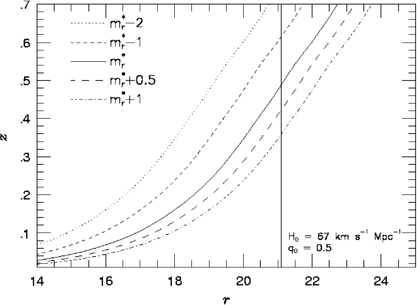
Figure 1: The magnitude-redshift relation for elliptical galaxies with $M^{*}_{r}=-21.52$. The survey limit is indicated by the vertical line at $m_{r}$ = 21.1.

To detect clusters at a given redshift, a photometric survey should be deep enough to sample sources significantly fainter than the characteristic luminosity at that redshift. Figure 1 shows the apparent magnitude-redshift relation for elliptical galaxies at different ranges around $m^{*}$. We use $M^{*}_{r}=-21.52$ (Paolillo et al., 2001) and assume clusters are dominated by early-type galaxies. The K-correction for elliptical galaxies is derived with the use of the spectral energy distributions from Coleman, Wu, & Weedman (1980), convolved with the DPOSS $r$-band filter. We adopt $m_{r}=21.1$ as the limiting magnitude of the survey, as indicated by the vertical line in Figure 1. If we assume that we need to go as deep as $m^{*}+1$ to detect a significant number of elliptical galaxies to identify a cluster over the background, then the survey limit lies below $z=0.4$. At $z\sim 0.5$ we are able to identify only the richest systems, which have a large number of galaxies brighter than $m^{*}$. We should keep in mind that these limits are valid for clusters composed entirely of early-type galaxies. The presence of late-type galaxies would render distant cluster members brighter as the K-correction effects are less strong.

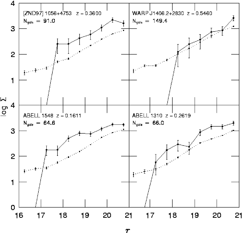
Figure 2: Differential magnitude distributions for four rich galaxy clusters with known spectroscopic redshifts. Cluster counts are shown as solid lines, while dotted lines show the local background counts. All counts are normalized to an area of one square degree.

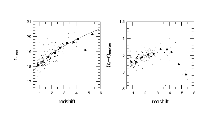
Figure 12: The mean galaxy magnitude $r_{mean}$ and median color $(g-r)_{median}$ for clusters as a function of spectroscopic redshift. The solid line shown in the left panel represents the empirical relation used to estimate redshifts for this work.

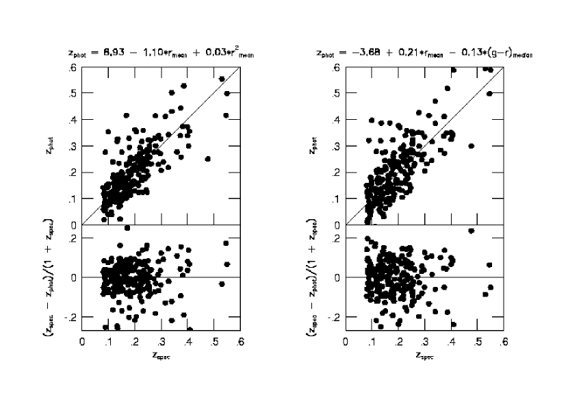
Figure 13: The photometric redshift estimate vs. spectroscopically measured redshift for 238 clusters. Residuals as a function of magnitude are shown in the bottom panel of each plot. We show photometric estimates based on only the mean magnitude (left panel), as well as both the mean magnitude and median color $(g-r)$ (right panel).

Figure 2 shows the differential magnitude distribution of galaxies within the projected area of four rich galaxy clusters (solid lines) with known spectroscopic redshifts and richnesses given by N_gals (§5.2). Field counts are also shown (dotted lines). All counts are normalized to one square degree. The shift of the luminosity function to fainter apparent magnitudes as we go to higher redshifts is obvious. However, it is clear from this figure that the cluster profile is easily differentiated from the background counts for these rich clusters to at least $z\sim 0.35$, being still over the background for $z\sim 0.5$ rich systems. Considering these two figures, along with the left panels of Figures 12 and 13 (where we show that the mean magnitude is generally well determined at $z\sim 0.5$) we, adopt $z\sim 0.5$ as a formal limit for the detection of rich clusters for the survey.

2.2 Field Selection

As mentioned above, the star-galaxy separation accuracy drops below the 90% level at $m_{r}>19.5$. Photometric errors and observing conditions also play a key role in the generation of an input catalog for our cluster search. To mitigate these effects, we apply a galactic latitude cut when selecting the DPOSS fields to be used. Additionally, we exclude fields based on their limiting magnitudes and seeing, as outlined below.

The plate catalogs used in this paper contain galaxies with $16\leq m_{r}\leq 21.1$. Initially, we ignored classification for faint objects ($m_{r}>19.5$), assuming that stars would add a constant background to the galaxy distribution at high galactic latitudes. However, this contribution is not expected to be mild. We therefore adopt a statistical approach to check the probability that a faint star is indeed a galaxy. This procedure is explained below.

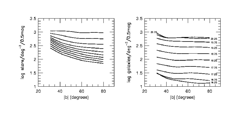
Figure 3: Star and galaxy counts as a function of galactic latitude for different magnitude bins. The left panel shows the star counts, while the right panel shows the galaxy counts. The magnitude bins are indicated in the right panel.

The first criterion to select DPOSS fields is the galactic latitude ($|b|$). We look for regions on the sky where density gradients as a function of $|b|$ are minimized. In these areas we assume that the stellar contamination (regardless of the actual level) represents a uniform background added to the galaxy distribution. Figure 3 shows the stellar (left panel) and galaxian (right panel) number counts for different magnitude bins as a function of galactic latitude ($|b|$). The magnitude bins are indicated in the right panel. All lines represent spline fits to the mean density from 375 DPOSS plates. There is a strong dependence on galactic latitude, mainly for low-$|b|$ fields ($|b|<45^{\circ}$), due to misclassified stars close to the galactic plane, with the increase in density due to stellar contamination in these low-$|b|$ fields.

Another issue is whether the Poissonian fluctuations in the number of stars misclassified as galaxies could affect the cluster detection. In order to estimate the magnitude of this effect, we computed the expected $\sqrt{N}$ fluctuations in the number of such misclassified stars within a typical cluster aperture, as functions of both magnitude and galactic latitude. We find that for $m_{r}<19$, the contamination is less than 0.1 star per cluster aperture, increasing to $\sim 2$ stars per cluster aperture at $m_{r}=20.5$. Thus, we conclude that the effect of such fluctuations is negligible for our purposes.

Based on Figure 3, we conservatively select only fields with $|b|>50^{\circ}$. This is motivated by the fact that in this latitude range we expect any contamination caused by stars to be approximately uniform. Nevertheless, we should still avoid high contamination levels. Initially, we decided to simply ignore classification for magnitudes fainter than $m_{r}=19.5$ (the star-galaxy classification limit). Unfortunately, in this magnitude range galaxy counts do not exceed star counts by a large margin. At $m_{r}=19.5$ the ratio of galaxy to star counts is expected to be only 1.3, increasing to 2.5 at $m_{r}=20.5$. If we ignore classification for objects with $m_{r}>19.5$, 30% of our catalog would consist of stars (misclassified as galaxies) at these magnitudes. Since $\sim$ 84% of all objects with $m_{r}<21.1$ have $m_{r}>19.5$, the overall expected stellar contamination would be $\sim 25\%$. To reduce this effect and generate object catalogs with statistically reliable galaxy counts, we opted for a statistical approach to assess the probability that faint stars are actually galaxies. This methodology was previously employed by P02 and Postman et al. (1998). The procedure consists of the extrapolation of the bright star counts ($m_{r}<18.5$) to fainter magnitudes. We can then compare the number of stars that should be in each magnitude bin to the actual value found in the DPOSS survey, computing the probability that a given star in a given magnitude bin is actually a misclassified galaxy. This function is applied to the DPOSS faint stars ($m_{r}>18.5$), having as a final product an object catalog with statistically reliable galaxy counts. The probability function (described below) is given by

$$P=5.16-3.2\times 10^{-3}r^{2}+4.97\times 10^{-5}r^{4}$$

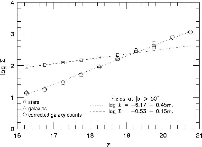
Figure 4: Star and galaxy counts at $|b|>50^{\circ}$. Stars are shown as squares and galaxies as triangles. The dotted line is the best fit to the bright galaxy counts extrapolated to $m_{r}=21$. The dashed line represents the bright star counts ($m_{r}\leq 18.5$) extrapolated to $m_{r}=21$. Circles represent the corrected galaxy counts out to $m_{r}=21$. Error bars (not shown here for clearness) are at the same level of the error estimates for field counts in Figure 2.

This effect is illustrated in Figure 4, where we plot the number counts for stars (squares) and galaxies (triangles) as a function of magnitude, to $m_{r}=20$, in bins of $0.5^{m}$. The dotted line is the best fit to the bright galaxy counts, extrapolated to $m_{r}=21$. The dashed line is the relation used to assess the probability given by equation (1); it is the best fit to the bright star counts ($m_{r}<18.5$) extrapolated to $m_{r}=21$. Equation (1) is derived from the comparison of the number of faint stars found in DPOSS to the expected value given by the dashed line relation. The corrected galaxy counts are shown as circles. These are only slightly higher than the observed counts (triangles) at $m_{r}=19.5$, in agreement with the 90% galaxy success rate at this magnitude. The circles are also well fit by the dotted line at faint magnitudes, demonstrating that the corrected counts are in agreement with the extrapolated galaxy counts from the brighter bins.

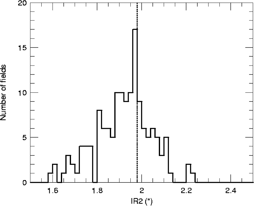
Figure 5: The intensity-weighted second moment of the light distribution for stellar objects (IR2) in the $r$-band is given as an indication of the quality of DPOSS fields. Its distribution is shown above for the well calibrated and high latitude DPOSS fields. We select fields with IR2 $<1.98^{\prime\prime}$.

We apply two additional criteria to select DPOSS fields for this survey. First, we restrict the cluster search to fields with good seeing. We use the intensity-weighted second moment of the light distribution on the red plate for stellar objects (IR2_r) as an indicator of the quality of the observations. Figure 5 shows the IR2_r distribution for $|b|>50^{\circ}$ fields. We use only fields with IR2_r $\leq 1.98^{\prime\prime}$ (close to the median value), as indicated by the vertical line in the plot. This is equivalent to seeing measures varying from 2.0^′′ to 2.5^′′. The poor seeing is a convolution of the atmospheric seeing, telescope optics, and the plate scanning process.

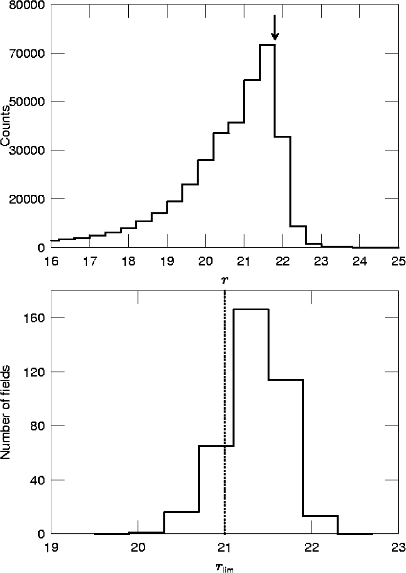
Figure 6: Typical magnitude distribution of a DPOSS field (top). The limiting magnitude is indicated by the arrow. In the bottom panel we show the distribution of limiting magnitudes for 375 DPOSS plates. We exclude fields with $m_{r,lim}<21$.

Finally, we exclude fields with limiting magnitudes brighter than $m_{r}=21$. The top panel of Figure 6 shows the $r$ band magnitude distribution for a typical DPOSS field. As in Picard (1991), we consider the magnitude limit to be the magnitude where the distribution starts to drop steeply (as indicated by the arrow). The bottom panel of the same figure shows the distribution of magnitude limits, with the chosen cut indicated by a vertical line at $m_{r}=21$.

To summarize, we select the best fields for this project based on three criteria. Initially we begin with 375 fields. Excluding fields with poor photometry and at $|b|<50^{\circ}$ leaves 146 fields, which is reduced to 109 after selecting those with IR2 $\leq 1.98^{\prime\prime}$. Finally we eliminated one field which has a bright magnitude limit, $m_{r}<21$. The final sample used for the cluster search thus comprises 108 fields distributed over the northern sky, providing an area coverage of $\sim 2,700$ square degrees.

3 Cluster Detection Algorithms

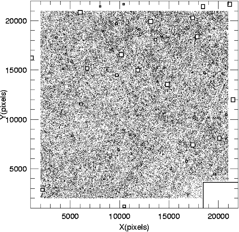
Figure 7: Galaxy distribution in DPOSS Field 444 ($\alpha=201.64^{\circ},~{}\delta=29.74^{\circ}$) for $16.0\leq m_{r}\leq 21.1$. Excised areas due to bright objects are indicated by rectangles. A cleaned path due to a satellite trail is visible in the lower right corner.

In Papers I, II and III we detected galaxy clusters using the DPOSS galaxy catalogs restricted to $m_{r}\leq 19.5$. At this limit, all real objects are detectable in both the $r$ and $g$ bands, so we require that all objects to $m_{r}=19.5$ must also have a counterpart in the $g$ band, to avoid spurious detections associated with satellite or airplane trails and plate defects. For the deeper survey presented here, this requirement is no longer practical. At the current limit of $m_{r}=21.1$ there are $J$ (blue) plates which are not as deep as the $F$ (red) plates, resulting in real objects detected only in the $r$-band which have no counterpart in the shallower $g$-band catalogs. We have therefore opted to use only the $r$-band when preparing the galaxy catalogs. As described in Djorgovski et al. (2004) this results in $\sim 10\%$ of $r$-band only detections being spurious; these are mainly associated with meteor and aircraft trails. We exclude such objects by fitting a linear relation to trails present in our galaxy catalogs and removing detections in the corresponding areas. Approximately 20% of plates require this special treatment. An example galaxy catalog for a plate with a cleaned trail (in the bottom right corner) is plotted in Figure 7. As in the previous papers, detections in the vicinity of bright objects (where our photometry fails) are also excised.

Another difference from the previous papers is the use of only the central part of each plate. We apply cuts in pixel coordinates, using only objects with 2000 $\leq X,Y\leq$ 21000 (out of the maximum 0 $\leq X,Y\leq$ 23040), resulting in catalogs of typically $\sim$ 116000 galaxies over an area of $\sim$ 25 square degrees (compared to 34 square degrees from Papers II and III). This is necessary to avoid the heavily vignetted areas near the plate edges. The mean galaxy density is $4.6\times 10^{3}$ galaxies per square degree (approximately six times higher than in Papers II and III). The survey covers $\sim 2,708\square^{\circ}$, containing $\sim 1.3\times 10^{7}$ galaxies.

In this paper two independent techniques are employed to detect galaxy clusters. One, the adaptive kernel technique (AK) (Silverman, 1986) was already used by our group (Papers I, II and III), while the second technique uses Voronoi Tessellation (VT). The main differences between the applications of these two methods to DPOSS data are:

(i)

The AK is applied only to the projected distribution of galaxies, while the VT method also incorporates magnitude information.

(ii)

As our goal in the present work is the detection of intermediate redshift rich clusters, the galaxy catalogs used by the AK contain only objects with 19 $\leq m_{r}\leq 21.1$. We expect to find clusters with luminosity functions spanning these fainter magnitudes and thus avoid low-$z$ clusters. Initially we planned to employ the VT technique using the same galaxy catalogs, but because we can use magnitudes to minimize background/foreground contamination, we opted for a brighter cut at $m_{r}=16$, instead of $m_{r}=19$, as detailed in section 3.1.

The next two sections present a brief description of both techniques applied to DPOSS data, with further detail in the references provided below.

3.1 The Voronoi Tessellation Technique

Considering a homogeneous distribution of particles it is possible to define a characteristic volume associated with each particle. This is known as the Voronoi volume, whose radius is of the order of the mean particle separation. Voronoi Tessellation has been applied to a variety of astronomical problems. A few examples are found in Ikeuchi & Turner (1991), Zaninetti (1995), El-Ad et al. (1996), Doroshkevich et al. (1997). Ebeling & Wiedenmann (1993) used Voronoi Tessellation to identify X-ray sources as overdensities in X-ray photon counts. Kim et al. (2002) and Ramella et al. (2001) looked for galaxy clusters using Voronoi Tessellation (VT). As pointed out by Ramella et al. (2001) one of the main advantages of employing VT to look for galaxy clusters is that this technique does not distribute the data in bins, nor does it assume a particular source geometry intrinsic to the detection process. The algorithm is thus sensitive to irregular and elongated structures.

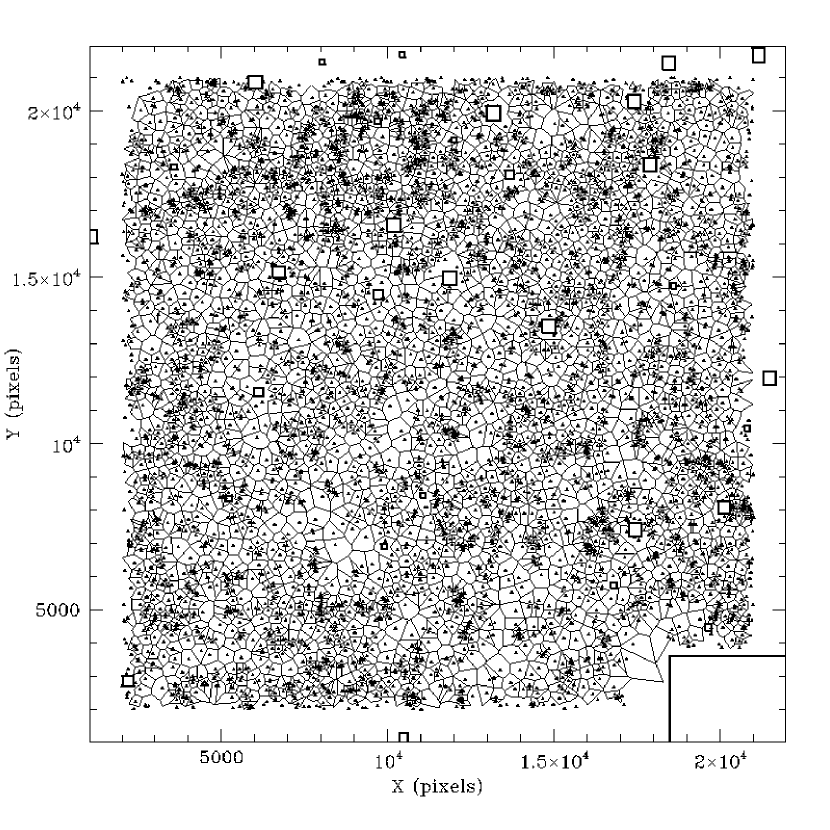
Figure 8: Voronoi Tessellation of galaxies with $17.0\leq m_{r}\leq 18.5$ in Field 444. Each triangle represents a galaxy surrounded by its associated Voronoi cell (indicated by the polyhedrals). Excised areas (due to bright objects) are shown as rectangles.

The parameter of interest in our case is the galaxy density. When applying VT to a galaxy catalog, each galaxy is considered as a seed and has a Voronoi cell associated to it. The area of this cell is interpreted as the effective area a galaxy occupies in the plane. The inverse of this area gives the local density at that point. Galaxy clusters are identified by high density regions, composed of small adjacent cells, i.e., cells small enough to give a density value higher than the chosen density threshold. An example of Voronoi Tessellation applied to the DPOSS field in Figure 7 is presented in Figure 8. For clarity, we show only galaxies with $17.0\leq m_{r}\leq 18.5$.

In order to detect galaxy clusters using Voronoi Tessellation we use the code employed by Ramella et al. (2001). It uses the triangle C code by Shewchuk (1996) to generate the tessellation. The code is designed to avoid the borders of the field, as well as the excised areas around saturated objects. The algorithm identifies cluster candidates based on two primary criteria. The first is the density threshold, which is used to identify fluctuations as significant overdensities over the background distribution, and is termed the search confidence level (scl). The second criterion rejects candidates from the preliminary list using statistics of Voronoi Tessellation for a poissonian distribution of particles (Kiang, 1996), by computing the probability that an overdensity is a random fluctuation. This is called the rejection confidence level (rcl). More details can be found in Ramella et al. (2001).

Kim et al. (2002) used a color-magnitude relation to divide the galaxy catalog into separate redshift bins, and ran the VT code on each bin. The candidates originating in different bins were cross-correlated to filter out significant overlaps and produce the final catalog. Ramella et al. (2001) follow a different approach, as they do not have color information. Instead, they use the object magnitudes to minimize background/foreground contamination and enhance the cluster contrast, as follows:

(i)

The galaxy catalog is divided into magnitude bins, starting at the bright limit of the sample and shifting to progressively fainter magnitudes. The step size adopted is derived from the photometric errors of the catalog.

(ii)

The VT code is run using the galaxy catalog for each bin, resulting in a catalog of cluster candidates associated with each magnitude slice.

(iii)

The centroid of a cluster candidate detected in different bins will change due to the statistical noise of the foreground/background galaxy distribution. Thus, the cluster catalogs from all bins are cross-matched, and overdensities are merged according to a set criterion (described below), producing a combined catalog.

(iv)

A minimum number (N_min) of detections in multiple bins is required in order to consider a given fluctuation as a cluster candidate. N_min acts as a final threshold for the whole procedure. After this step, the final cluster catalog is complete.

Ramella et al. (2001) applied their algorithm to one of the Palomar Distant Cluster Survey (PDCS) galaxy catalogs. They divided this deep data into bins of two magnitudes, starting with $18.0\leq V_{4}\leq 20.0$ and shifting to fainter bins in steps of 0.1 mag down to the detection limit ($V_{4}=23.8$). This procedure resulted in 39 bins. They adopted scl = 0.80 and rcl = 0.05 to select fluctuations in each bin. They then merged candidates whose centers had a projected distance equivalent to $d_{12}\leq 0.3min(R_{1},R_{2})$, where $R_{1}$ and $R_{2}$ are the radii of any two candidates being compared. Finally, they kept only candidates with N${}_{min}=5$. While not stated in their paper, they further merged clusters whose radii overlap.

When applying this algorithm to DPOSS data we tested different bins and step sizes. As with the PDCS galaxy catalog, we span five magnitudes, but in a brighter regime and with larger photometric errors. We adopt a bin size of 1.5 magnitude and a step size of 0.2 magnitudes. This step size is comparable to the photometric error at $m_{r}=19.5$. A wider magnitude bin could be used, but would significantly decrease the number of steps. A narrower bin would result in a low number of cluster galaxy counts per bin. We thus have 19 bins spanning the range $16\leq m_{r}\leq 21.1$. As seen in Figure 2, 1.5 magnitudes is a reasonable range to see clusters over the background.

The threshold given by scl selects overdensities above a given galaxy surface density. Due to the non-uniform nature of plate data and the effects of large scale structure, we do not use a single threshold for the 108 different plates used in this project. Instead, we maintain rcl fixed at 5%, but allow scl to vary. The VT code is run for each DPOSS field varying scl from 0.78 to 0.92 (in steps of 0.02), instead of adopting a fixed value of 0.80 as in Ramella et al. (2001).

The percolation analysis we apply to the cluster candidate catalogs from different bins is similar to that of Ramella et al. (2001). However, the optimal parameters found for DPOSS data are slightly different. We chose $d_{12}\leq 0.8min(R_{1},R_{2})$ and N${}_{min}\geq 3$, plus a final merging of structures whose separation is smaller than the radius of the largest neighboring candidate. These values are selected based on the redshift range over which we are detecting clusters, and the nature of our data. The PDCS data used by Ramella et al. (2001) has no nearby large clusters, as the data covers only 1 $\square^{\circ}$ and was designed to avoid bright objects and low-$z$ clusters. Tests done with a smaller matching radius show that many nearby clusters would be broken into subcomponents. The use of larger radii can incorrectly associate adjacent clusters into a single candidate. The choice of N${}_{min}\geq 3$ is explained in the next section, as it depends on the number of false clusters (the contamination rate) produced for each DPOSS field. The choice is sensible given that we have half the bins (19 compared to 39) of Ramella et al. (2001).

As with the AK, the VT is optimized based on simulations of the background galaxy distribution, where we apply the VT code to both these simulated fields and real DPOSS fields. These techniques are described in §4.

3.2 The Adaptive Kernel Technique

We use a two-stage version of the adaptive kernel technique, which generates an initial density estimate on a fixed grid. It then applies a smoothing kernel whose size changes as a function of the local density, with smaller kernels at higher densities. Finally, a density map is generated for each DPOSS field and SExtractor is used to locate overdensities on this map. More details can be found in Papers I and II and in Silverman (1986). The galaxy catalogs used as input to the AK have galaxies at 19 $\leq m_{r}\leq$ 21.1. In the previous NoSOCS papers the pixel scale adopted for the density maps was 1 pixel = 60^′′. For the current project, we aim to detect distant (generally compact, low contrast) structures. We therefore require higher resolution for the density maps, which are here generated with a scale of 1 pixel = 10^′′.

Gladders & Yee (2000) utilize a more powerful technique to detect clusters, with a color-magnitude relation as a filter to minimize contamination from foreground sources. However, the surface density of objects is evaluated in a similar way to ours. The main difference is that they use a simple fixed kernel, which is applied independently to each color slice. They argue that our estimator might not be optimal because the AK tends to resolve high density regions in the data. Based on cluster simulations, we show (see Figure 1 in Paper II) that with the proper choice of the initial kernel size we do not divide nearby rich clusters into subcomponents, while remaining sensitive to low contrast structures (poor and close, or rich and distant). A simple fixed kernel technique may be inappropriate in our situation, as it is not simultaneously sensitive to clusters of different richness classes at different distances.

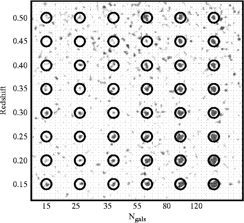
Figure 9: Density map of a simulated background galaxy distribution with 48 artificial clusters inserted. The initial kernel adopted has a 260^′′ radius. Artificial clusters are marked by circles. Each row represents a different redshift ($z=$0.15, 0.20, 0.25, 0.30, 0.35, 0.40, 0.45, 0.50), increasing from bottom to top. Richness increases from left to right (N${}_{gals}=15,25,35,55,80,120$).

In Papers II and III we adopted an initial kernel of $500^{\prime\prime}$ radius to look for lower redshift clusters ($z<0.3$) with our brighter galaxy catalogs. As before, we use simulated clusters to test the kernel size for the fainter catalogs at $19\leq m_{r}\leq 21.1$. The optimal value found is $260^{\prime\prime}$. Figure 9 shows a density map generated with a $260^{\prime\prime}$ radius initial kernel. 48 artificial clusters of six richness classes (N${}_{gals}=15,25,35,55,80,120$) at 8 different redshifts ($z=$0.15, 0.20, 0.25, 0.30, 0.35, 0.40, 0.45, 0.50) are inserted. Clusters are marked with circles and each column represents a different richness class (increasing from left to right), while each row is a different redshift (increasing from bottom to top). We can see that our choice for the initial kernel radius does not break up the nearby clusters, while it is still sensitive to distant rich structures.

After generating a density map for each DPOSS field we then run SExtractor to detect high density peaks, which we associate with cluster candidates. Simulated background distributions are used to optimize SExtractor parameters (see section 4). As in Papers II and III, each DPOSS field is optimized independently.

4 Contamination and Optimization of the Algorithms

As stated in Paper II, contamination by random fluctuations in the galaxy distribution and chance alignments of galaxy groups can seriously affect any cluster catalog. This problem is exacerbated in a survey like this one, which lacks color information to minimize background/foreground contamination (Gladders & Yee, 2000; Goto et al., 2002).

The most common methods to estimate how much a given catalog is affected by these factors use simulated background distributions. A simple random distribution with the same number density as the original field would underestimate contamination. A background constructed this way reproduces random fluctuations, but not the large scale structure present in a given field. Goto et al. (2002) tested three different backgrounds, where they: (i) shuffled the positions without touching colors; (ii) shuffled the colors, but did not touch the positions; (iii) shuffled the colors and smeared the positions. That was done specifically for their algorithm, which makes use of the extensive multicolor information from the SDSS. Algorithms which do not make use of color usually have their contamination estimate based on a shuffled background (Lobo et al., 2000), a Poissonian galaxy distribution (Ramella et al., 2001), or on a distribution generated with the same angular correlation properties as the real field (P02; Paper II; Gilbank 2001).

For this project we have tested four types of simulated backgrounds: (i) a Raleigh-Levi (RL) distribution (P02; Paper II); (ii) a shuffled background; (iii) a randomized galaxy distribution; and (iv) a smeared background. In the latter case galaxy magnitudes are maintained, while the positions are randomly redistributed within 7^′ of their original ones. Goto et al. (2002) adopted 5^′ for the smearing scale. They found the contamination rate evaluated with this background to be extremely high in comparison to the other ones tested. As described below, we test the optimization of our algorithms at the 5% and 10% contamination levels. Commensurate with the results of Goto et al. (2002), we find that it is not possible to optimize the AK or VT at these levels with the smeared background, and we have therefore abandoned it in the tests described below. The RL distribution is intended to simulate galaxy distributions with an angular two point correlation function similar to that of the real data.

A variety of methods have been used to minimize the number of false detections (N_false) in a simulated background distribution when optimizing cluster detection algorithms. The number of false clusters per square degree has been presented as an indicator of how low contamination effects could be for a given catalog. However, as the photometric depth of catalogs varies, so will the absolute number of false detections. Thus, the contamination rate ($C$ = N_false/N_real) has been more commonly used to optimize cluster detection algorithms. N_false gives the number of false detections in a simulated distribution, while N_real is the number of detections in the real galaxy distribution. Optimal detection thresholds are achieved for the highest recovery rate allowed at a given contamination level.

We performed tests using 20 DPOSS fields and compared the results obtained at the 5% and 10% contamination levels. For the VT algorithm the threshold is given by a combination of scl and N_min (see section 3.1). We chose not to fix the values of these parameters; rather, they are determined independently for each field. For a given DPOSS field the best option might consist of a high value of scl with a low number of minimum detections, while the reverse could be true in other cases.

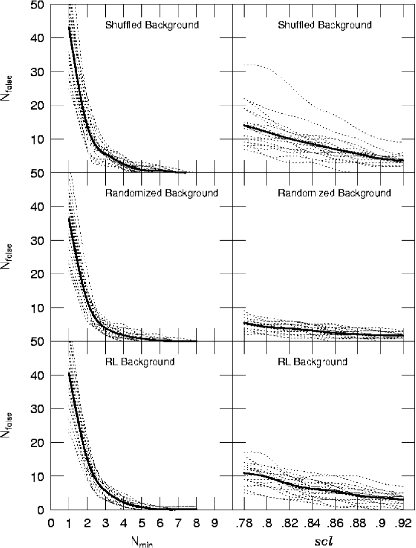
Figure 10: Comparison of the number of false detections using an RL background distribution, a randomized background, and a shuffled background. The dotted lines show the variation of N_false with N_min (left panels) and scl (right panels) for 20 different DPOSS fields, while the solid line shows the mean variation.

Figure 10 compares the variation of N_false with N_min (left panels) and scl (right panels) for the RL, randomized and shuffled distributions. Each dashed line represents the variation of N_false for one of the 20 DPOSS plates tested. The solid line shows the mean variation on each panel. In order to compare the performance of the three different backgrounds we use N_false, as it is the only parameter to vary when estimating $C$. The dispersion is basically the same for all distributions in the left panels, being slightly higher when the shuffled background is used. The right panels indicate the contamination estimate is lowest, and least sensitive, to the randomized background. The RL and shuffled distributions show similar results to each other (except for two outliers in the latter case). This suggests that the randomized background underestimates the contamination. The RL is a model representation of the angular distribution in a galaxy field. N_false smoothly decreases as we move to higher thresholds (given by N_min and scl). However, the RL distribution might not properly represent variations in high density fields. We expect the correlation properties to vary for different DPOSS fields as they have different galaxy densities (Maddox, Efstathiou & Sutherland, 1996). As a full analysis of the correlation properties of all DPOSS fields is beyond the scope of this project, we decided not to use the RL distribution for this paper. Instead, the shuffled background is adopted to optimize our algorithms. It shows no large differences relative to the RL distribution, and is a model-independent representation of the background.

We then generate a shuffled catalog (simply repositioning all galaxies within a DPOSS field and keeping the magnitudes) and run the VT on this list, which gives N_false. The VT is also run on the real catalog, yielding N_real. Each field is optimized for the values of scl and N_min which yield the maximum N_real, while keeping the contamination rate fixed at $C\sim 5\%$. Note that 5% is a lower limit for contamination effects. A full assessment requires a spectroscopic follow-up.

The strategy adopted to optimize the AK algorithm is basically the same as for the VT. We take the shuffled catalogs generated for the VT optimization and trim them to the appropriate magnitude limit ($19\leq m_{r}\leq 21.1$) adopted for the AK. We run the AK on these catalogs as well as the original data to generate density maps for each. SExtractor is used to detect overdensities on these maps.

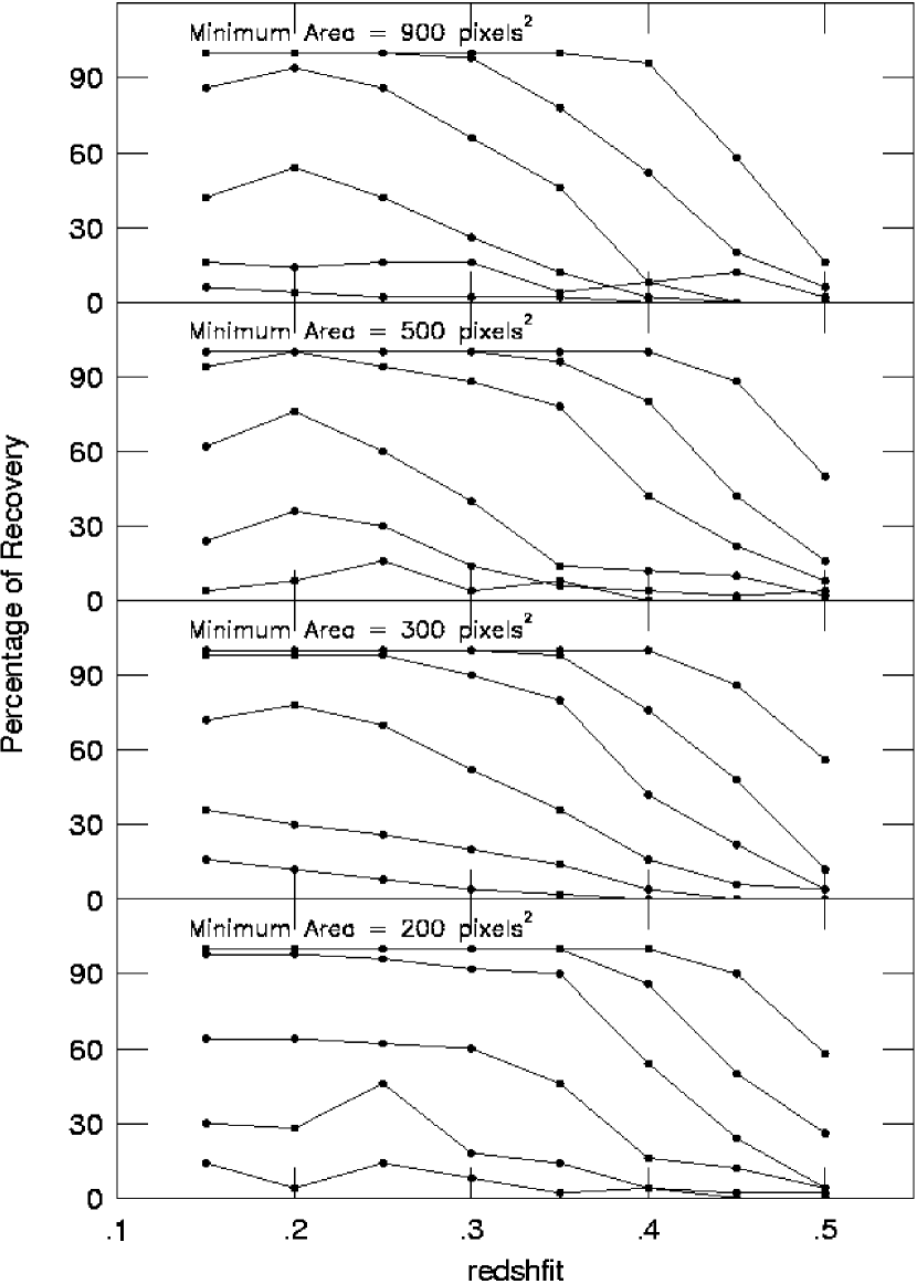
Figure 11: The selection function with the AK code for 4 different values of the minimum area: 200, 300, 500 and 900 pixels². Within each panel, the lines represent different richness (N${}_{gals}=15,25,35,55,80,120$), increasing from bottom to top.

The parameters that give the final optimization of the AK are the minimum area and the threshold required for a detection when running SExtractor. The minimum area gives the minimum number of pixels a candidate must have, while the threshold gives the minimum number of galaxies per square degree. We vary the threshold from 3000 to 9000 galaxies per $\square^{\circ}$. Tests in a broader range for 20 plates show that the optimal threshold is always found within these values. Four different values are tested for the minimum area: 200, 300, 500 and 900 pixels². In order to choose the optimal value for the minimum area we evaluate the selection function with these four different values (see Figure 11). We find that 200 and 300 pixels² produce similar results, with a slightly higher recovery rate in the former case. Going to 100 pixels² does not result in any improvement. Thus, we adopted 200 pixels² as the minimum area for all DPOSS fields when running SExtractor. As stated above the threshold is optimized for each plate.

5 The Cluster Catalogs

The main goal of this project is to provide a catalog with rich galaxy clusters to intermediate redshift for follow-up studies. In order to be able to select subsamples from the main catalog we provide some basic properties, such as redshift and richness, for the cluster candidates. When estimating these two quantities we use similar, but not identical, techniques to those employed in Papers II and III. However, we face a variety of challenges for the current project. For instance, the photometric errors are large in the magnitude range utilized here, which also affects color measures; the number of clusters with known spectroscopic redshift to be used as a training sample is small when we go out to $z\sim 0.5$; the $(g-r)$ color is not useful for $z\gtrsim 0.4$ clusters (as the 4000 Å break shifts from $g-r$ to $r-i$); and the blue plates do not necessarily go as deep as the red ones.

In §5.1 and §5.2 we describe our efforts to estimate redshift and richness for the cluster candidates. A visual inspection is employed in §5.3 to eliminate obvious false clusters associated with bright stars, nearby galaxies and groups. A combined version of the VT and AK cluster catalogs is presented in section 5.4.

5.1 Photometric Redshifts

An empirical relation based on the mean $r$ magnitude and median $(g-r)$ color was successfully used to estimate redshifts for the NoSOCS clusters (Papers I, II and III). Here, we assume these same properties are strong indicators of the redshift of a cluster. However, this paper employs significantly different methodologies, and it is not clear a priori if useful photometric redshift estimation is possible using the faintest DPOSS data.

The main differences with respect to the photometric redshift technique employed in Paper II are: (i) The galaxy catalogs used here have a statistical correction applied to them (section 2.2), which gives rise to a $\sim 15\%$ difference in number counts around $m_{r}=20$; (ii) counts were previously done at 15 $<m_{r}<$ 20, while now we count galaxies at 16 $<m_{r}<21.1$; (iii) we now adopt local estimates for the background counts, instead of taking these estimates from the whole area of each plate. Additionally, we tested different counting radii (0.50, 0.75, 1.0 and 1.5 h^-1 Mpc), and found that 1.0 h^-1 Mpc produces the fewest outliers and minimizes the overall dispersion.

The first step towards the determination of photometric redshifts is the compilation of a list of clusters with measured spectroscopic redshifts. Unfortunately, there are few clusters with spectra taken at $z>0.3$, which biases our sample to low-$z$ clusters. Our calibration sample consists of 238 clusters over the $\sim 2,700$ square degrees of this survey, taken from Struble & Rood (1999), Holden et al. (1999), Vikhlinin et al. (1998), Carlberg et al. (1996), and Mullis et al. (2003). In comparison, the training sample for Paper II had 369 clusters, over a narrower redshift range.

We proceed as follows: each of the 238 clusters with known spectroscopic redshift has the number of galaxies as a function of magnitude (N_r) and color (N_(g-r)) determined. These counts have the local background counts subtracted, resulting in a determination of the net cluster counts as a function of both color and magnitude. The mean $r$ magnitude ($r_{mean}$) and median color ($(g-r)_{median}$) is then computed for each cluster. Then we bin the colors and magnitudes in redshift bins of $\Delta z=0.05$, calculating the mean $z_{spec},r_{mean}$ and $(g-r)_{median}$ for each bin (see Figure 12). These values are used to derive two empirical relations for redshift estimation. The first uses only $r_{mean}$, while the second uses both $r_{mean}$ and $(g-r)_{median}$.

In Figure 12 we show the dependence of the estimated values of $r_{mean}$ and $(g-r)_{median}$ on spectroscopic redshift. As expected, colors are well behaved to $z\sim 0.4$. At higher redshifts we expect the $(g-r)$ color to remain approximately constant, as the 4000Å  break shifts from the $(g-r)$ color to $(r-i)$. However, we see that the $(g-r)$ estimate becomes meaningless for $z\gtrsim 0.4$. Two factors contribute to this color mismeasurement. First, there is incompleteness in the J (blue) catalogs. As seen in §2.2, the field selection is based only on the F (red) plates. We select only those F plates which go as deep as $m_{r}=21$, but the corresponding blue plates might not be equally deep. Fainter than $m_{r}\sim 19.5$ the number of two-band detections drops steeply, reaching $\sim 70\%$ at $m_{r}=21$. For Papers I, II and III the magnitude limit of the galaxy catalogs ($m_{r}=19.5$) allowed us to require a $g$-band detection when generating a galaxy catalog for the cluster search. This is not possible for the current survey. The second factor contributing to color mismeasurement is the possible contamination from stars at faint magnitudes.

In Figure 13 we compare the photometric and spectroscopic redshifts from the two relations discussed above, using only magnitude (left panel) and both color and magnitude (right panel). We find the dispersions to be similar, being slightly higher when we include colors to evaluate $z_{phot}$. As the color information does not significantly improve the photometric redshift estimate (using our data), we estimate redshifts using only $r_{mean}$. The fitted relation is

$$z_{phot}=8.93-1.10\times r_{mean}+0.03\times r^{2}_{mean}$$

with a dispersion in redshift of $\Delta z=0.052$. These errors are comparable to those of other techniques which rely solely on magnitudes for redshift estimation, such as the matched filter.

If we have no a priori knowledge of the cluster redshift, it must be determined iteratively. We choose an initial guess of the redshift ($z_{start}=0.15$), and compute $r_{mean}$ and $(g-r)_{median}$ based on the cluster corrected counts within 1.0 h^-1 Mpc, apply the empirical relation derived above and derive a photometric estimate of $z$. We then iterate this procedure until it converges, adjusting the radius in each iteration.

Using the 238 clusters with known $z_{spec}$, we tested four different starting redshifts ($z_{start}=0.05,0.10,0.15,0.20$). We find the estimates to have almost no dependence on the initial redshift. For instance, when comparing the results with $z_{start}=0.05$ and $z_{start}=0.15$, we find that $Q_{sigma}$ is $(z_{0.15}-z_{0.05})/(1+z_{0.15})=0.005$. We chose to use $z_{start}=0.15$, as it results in fewer outliers.

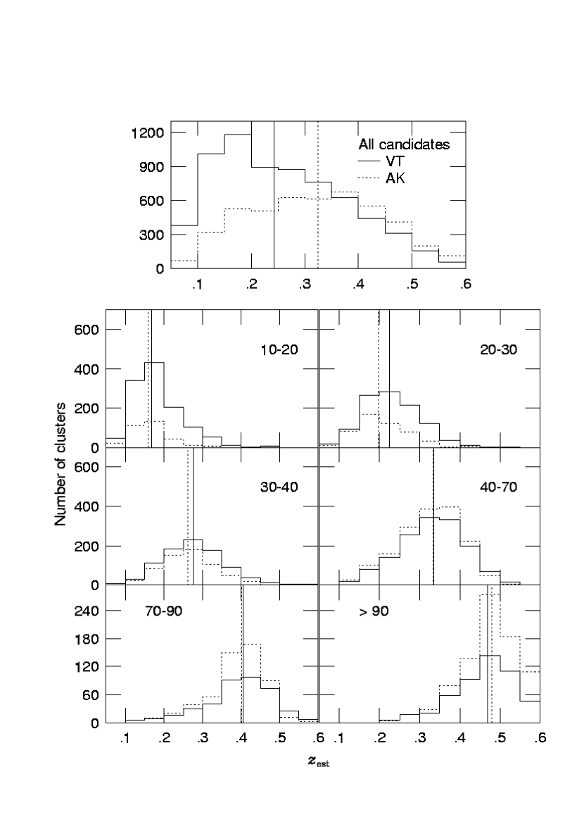
Figure 14: The estimated redshift distribution in different richness ranges and for the whole sample (top panel). The richness (N_gals) range is indicated in all panels. The median redshift is also indicated for the VT (solid line) and AK (dotted line) candidates.

Figure 14 shows the redshift distribution for different richness classes using both the AK and VT. The redshift cutoff in each case is generally in agreement with that seen in the selection functions (§6).

5.2 Richness Estimates

Richness is evaluated in a similar manner to Papers II and III. We describe below all the steps in the richness determination, pointing out the minor differences from the previously employed procedure. We proceed as follows:

1. We count the number of galaxies at $16.0\leq m_{r}\leq 21.0$ within 1.0 h^-1 Mpc of the cluster center. The background counts in the same range are evaluated locally, scaled to the cluster area, and subtracted, yielding the background-corrected cluster counts (hereafter N_corr). In the previous papers the magnitude range was $15.0\leq m_{r}\leq 20.0$ and the background was estimated from the whole plate.

2. We run a bootstrap procedure with 100 iterations. In each iteration, we randomly select N_corr galaxies at $16.0\leq m_{r}\leq 21.0$, within 1.0 h^-1 Mpc. Each galaxy has its apparent magnitude converted to an absolute magnitude. As with the artificial clusters (§6), we consider the clusters to be composed of 60% early-type and 40% late-type galaxies. When transforming to absolute magnitudes, we simply use elliptical K-corrections for 60% of the objects, and Sbc K-corrections for the remainder. We then count the number of galaxies between M${}^{*}_{r}$-1 and M${}^{*}_{r}$+2, where M${}^{*}_{r}$ = -21.52 (Paolillo et al., 2001). The mean value from the 100 iterations is computed, yielding the cluster richness N_gals, which can be decomposed into 40% Sbc galaxies (N_gals,Sbc) and 60% ellipticals (N_gals,E). If the cluster has a redshift such that M^∗-1 to M^∗+2 is fully sampled in the range $16.0\leq m_{r}\leq 21.0$, then the procedure is finished here. Otherwise we have to apply a correction factor to the richness estimate (N_gals), as described in step 3.

3. If the cluster is either too nearby or too distant, then M^∗-1 $<$ M₁₆ or M^∗+2 $>$ M₂₁, respectively, where M₁₆ and M₂₁ are the bright and faint absolute magnitude limits corresponding to $m_{r}=16.0$ and $m_{r}=21.0$. In practice these limits are different if a given galaxy is considered to be elliptical or spiral, due to the differing K-correction factors. Whenever M^∗-1 to M^∗+2 does not lie within M₁₆ and M₂₁ we apply correction factors for the richness estimate, defined as:

   $$\gamma_{1}={\int_{M_{r}^{*}-1}^{M_{r}^{*}+2}\Phi(M)dM\over\int_{M_{16}}^{M_{r}^{*}+2}\Phi(M)dM}$$

   $$\gamma_{2}={\int_{M_{r}^{*}-1}^{M_{r}^{*}+2}\Phi(M)dM\over\int_{M_{r}^{*}-1}^{M_{21}}\Phi(M)dM}$$

   We call $\gamma_{1}$ and $\gamma_{2}$ the low and high magnitude limit correction factors. Actually, each of these correction factors are evaluated twice, once for the magnitude limit for elliptical galaxies and the other for late-types. Whenever necessary, one of the above factors (as we span 5 magnitudes it is impossible to simultaneously miss both the bright and faint end) is multiplied by N_gals,E and/or N_gals,Sbc.

The main differences between steps 2 and 3 in this work relative to the procedure adopted for the previous NoSOCS papers lie in the assumption that the cluster is not totally composed of elliptical galaxies, and that we consider a correction factor to the lower magnitude limit.

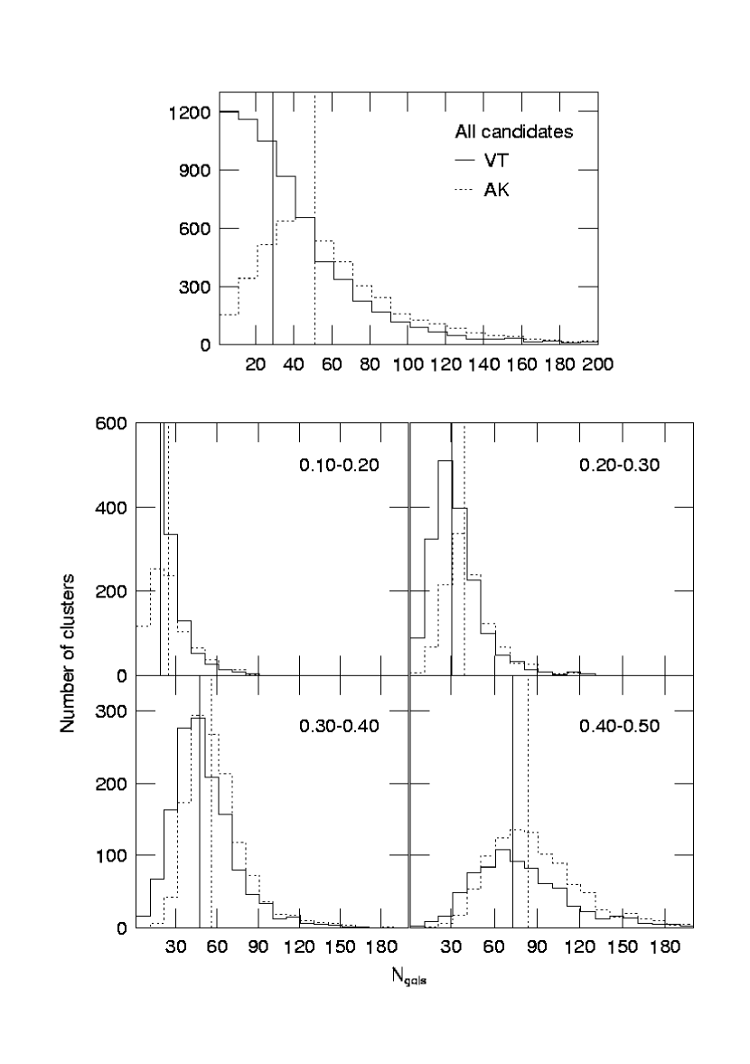
Figure 15: The richness distribution in bins of estimated redshift and for the whole sample (top panel). The redshift bins are indicated in each panel, as well as the median richness, which is indicated by the vertical lines (solid for the VT candidates and dotted for the AK).

In Figure 15 we show the richness distribution for the VT and AK cluster candidates for different redshift bins. The top panel shows the richness distribution for the entire sample. Further considerations related to redshift and richness estimates are discussed in section 8, where we compare the current catalog to the previous NoSOCS cluster catalog and to other surveys.

5.3 Elimination of Spurious Cluster Candidates

Before combining the VT and AK cluster catalogs we perform a visual inspection of the cluster candidates to eliminate obvious false clusters. Similar procedures were previously adopted by Kim (2001) and Goto et al. (2002). While inspecting the candidates we realized that many of them were associated with bright stars, and some with nearby bright galaxies and groups, globular or open clusters, plate defects, trails, etc. Thus, we decided to try to eliminate most of these false clusters in an automated fashion.

The major source of spurious detections is bright objects which were missed when generating the list of bad areas to be excised. In some cases, the object was removed, but the excised area was not large enough. We therefore decided to compare the cluster candidate positions to a bright star catalog. We used the Tycho-2 catalog (H$\phi$g et al., 2000), which is $\sim$ 90% complete to $V\sim 11.5$.

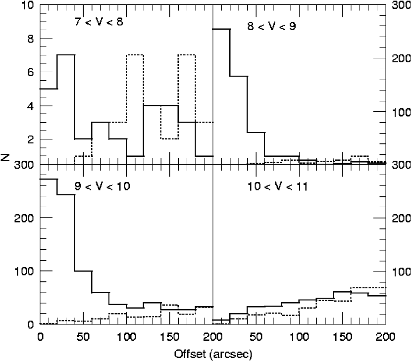
Figure 16: Offset distribution between Tycho-2 stars and cluster candidates (solid lines). The dotted lines represent the offset distribution using a mock star catalogue. The magnitude ranges are indicated on each panel.

Figure 16 shows, for 4 different magnitude bins, the distribution of offsets (in arcsec) between Tycho-2 stars and the nearest cluster candidate. The solid lines show the real offset distributions, while the dotted lines show the offset distribution between a mock star catalog and the cluster catalog. At 8 $<V<$ 10, almost all stars are associated with a cluster candidate within $120^{\prime\prime}$. Our photometry fails for these bright stars, which gives rise to a large number of faint, spurious detections in the halos of these objects. These spurious objects generate overdensities detected as cluster candidates. The catalogs presented in Papers I, II & III did not face this problem as most of these spurious detections are fainter than $m_{r}=19.5$, and do not have counterparts in the $g$-band. For the single band galaxy catalog utilized here, the elimination of bright objects turns out to be a serious issue.

We use the above information to clean our cluster catalog in a semi-automated fashion. From the inspection of offset distributions in different magnitude bins, we selected a minimum offset between a star and a cluster candidate (in each magnitude bin) to exclude the cluster as a false detection, and a function is interpolated to these minimum offsets as function of magnitude.

$$\Delta\theta_{min}=185+0.37\times(V^{2})-0.01\times(V^{4})$$

This function gives the minimum separation (in arcsec) a given cluster candidate must have from a star of a given V magnitude to be retained in the catalog. If the separation is smaller than this value, the candidate is excluded. Adopting this procedure, we eliminated 1031 VT and 1303 AK candidates. We further compared the cluster candidates to lists of bright galaxies, and globular and open clusters, which resulted in the elimination of a few more candidates. Finally, we visually inspect all the remaining candidates to exclude any associated with plate defects or trails. The total number of eliminated cluster candidates is 1602 ($\sim 17\%$) and 1748 ($\sim 27\%$) for the VT and AK catalogs, respectively. Note that as the detection codes were optimized to produce 5% contamination, reducing the number of real candidates by 20% results in an increase of the contamination rate to $C$ = N_false/N${}_{real}\sim 6\%$.

5.4 The Northern Sky Optical Cluster Survey (NoSOCS) High-Redshift Catalog

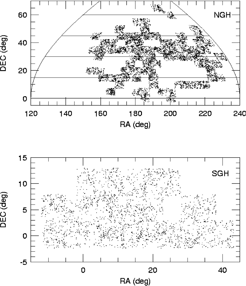
Figure 17: The sky distribution in equatorial coordinates for the combined AK-VT catalog (9,956 candidates). The region covering the northern galactic hemisphere is shown in the top panel, while the bottom panel shows the southern galactic hemisphere.

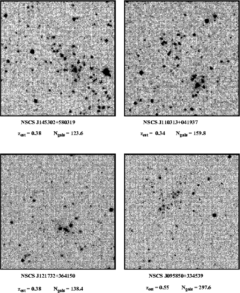
Figure 18: Examples of intermediate redshift rich clusters candidates detected in DPOSS. Images are 250^′′ on a side. NSCS J145302+580319 = Abell 1995 at $z_{spec}=0.32$; NSCS J110313+041937 was not previously catalogued; NSCS J121732+364150 = RX J1217.5+3641; NSCS J095850+334539 = ZwCl 0955.8+3401. Matches were found in NED using a search radius of 3 arcmin.

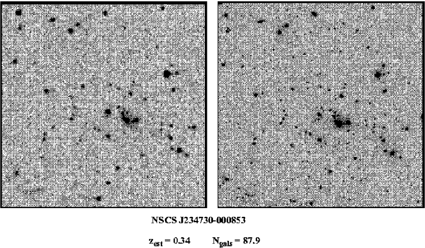
Figure 19: Candidate NSCS J234730-000853, also found by the CE method (Goto et al., 2002), with an estimated redshift from SDSS data of $z_{est}=0.24$. The left panel shows a DPOSS F-plate image, while the right panel shows a CCD image taken at the Palomar 60^′′ telescope. Images are 250^′′ on a side. This figure demonstrates the difficulty of visually confirming distant rich clusters from DPOSS plates.

The NoSOCS supplemental catalog presented here covers $\sim$ 2,708 $\square^{\circ}$ and originates from two cluster detection algorithms. The catalog contains 9,956 cluster candidates, which translates into a surface density of $\sim$ 3.7 clusters per square degree. The median estimated redshift of the AK clusters is 0.32, and is 0.24 for the VT clusters. The median richness is N_gals = 51.2 for the AK and N_gals = 29.3 for the VT. The sky distribution for the combined AK-VT cluster candidates is shown in Figure 17, for the regions in the northern galactic hemisphere (NGH) and southern galactic hemisphere (SGH). Examples of rich and distant clusters detected by the VT and AK codes are shown in Figure 18. The images are taken from the DPOSS F plate and span 250^′′ on a side. However, the low quality of the plates makes it difficult to visually identify most of these distant clusters. Figure 19 compares a cluster candidate imaged with a CCD at the Palomar 60^′′ telescope with its corresponding DPOSS F plate image.

The combined cluster catalog with 9,956 candidates is presented in Table 1, which is sorted by RA. In this printed version we present a sample of clusters with $0.4\leq z_{est}\leq 0.5$ and N${}_{gals}\geq 60.0$ (using the AK estimates). A complete version of this table can be found online at http://dposs.ncsa.uiuc.edu/ and the associated mirror sites. The table is organized as follows: column 1 gives the cluster name, where the convention is NSCS Jhhmmss+ddmmss (the second “S” in the name stands for supplemental); columns 2 and 3 give the RA and Dec in decimal degrees (J2000); the redshift estimates are shown in columns 4 (AK) and 5 (VT). Entries are set to zero whenever the corresponding estimator failed or if the candidate was not detected by that algorithm. Columns 6 and 7 present the richness estimates. The few candidates with redshift estimates greater than 0.6 (less than 40 clusters for each algorithm) are marked with the string “—” and have their richness set to zero. A few other candidates with the N_gals estimate greater than 400 (less than 10 clusters on each case) have their richness set to zero. We decided to keep redshift estimates at $0.5\leq z_{est}\leq 0.6$ instead of setting high-z estimates to a given value, such as $z=0.5$ (as done by Kim (2001)), and accumulate candidates in the last redshift bin. Column 8 has the plate number, while the codes that retrieved the cluster are listed in column 9. This column has “A” for the AK code, “V” for the VT and “AV” for both. We also provide (electronically) lists of bad areas used, as well as some other useful information for the reader. Cluster candidates found within 500^′′ of the plate edges (nearly two times the size of the initial kernel for the AK) are marked with an “*” in the last column. There are 333 candidates in these regions ($\sim$ 3% of the total sample); they are marked because their proximity to a plate edge may affect the local density estimate.

6 The Selection Function

In order to estimate the completeness of this catalog, we evaluated the selection function (SF) for a small number of DPOSS fields. Unlike Papers II and III, we do not perform a complete field-by-field analysis of the SF. However, it is important to note that for statistical studies such as the estimation of the space density and mass function of clusters, the SF should be evaluated individually for each field. The SF measurements presented here provide an approximate completeness estimate, and are used to check for possible improvement in the recovery rate for rich clusters when allowing a higher contamination level. In addition, the SF is useful for determining if the estimated redshift distributions shown in Figure 14 are realistic. Finally, in the richness and redshift regime where we predict our catalog to be nearly complete, we expect to find good agreement with other catalogs of rich clusters spanning the same volume. Comparisons to such catalogs are presented in §8.

The most common technique to evaluate the selection function makes use of artificial clusters. These are inserted in a background distribution and their recovery rate as a function of richness and redshift gives the SF. However, there are three major complicating factors:

1. The background used for completeness tests should not be the same as the one used for the optimization of the algorithm. As shown by Goto et al. (2002) and in Paper II, a simulated background overestimates the completeness rate. The real background distribution should be used instead.

2. When randomly placing artificial clusters in the background distribution we must avoid bad areas (due to saturated objects), as well as the positions of cluster candidates, as done by P02 and in Paper II. A simulated cluster located in the vicinity of a real cluster has its recovery probability changed from what it would be in a region devoid of clusters (which is more likely to be a background region). In this way we avoid the bias in the detection rates discussed by Goto et al. (2002).

3. The background plus artificial clusters galaxy catalog must have the same number density as the real field, as the optimal threshold was obtained with the original number density. Galaxies from rich artificial clusters can increase the number density of the field by a few percent.

We generate sets of 48 simulated clusters with 6 different richness classes (N${}_{gals}=15,25,35,55,80,120$) and placed at 8 different redshifts ($z=0.15,0.20,0.25,0.30,0.35,0.40,0.45,0.50$). These clusters are placed at random locations within a field; if it falls on a bad area or cluster candidate, a new position is chosen. We also preserve the same number of objects as in the original field by randomly removing the same number of galaxies from the original catalog as are inserted with the artificial clusters. This procedure is repeated 50 times.

For both the AK and VT methods we use a 0.75 h^-1 Mpc radius when comparing the input and output positions (this choice is explained below). An example of the selection function obtained for a DPOSS field with the VT code is shown in the middle panel of Figure 20. The SF for the AK code with the same field is shown in the bottom panel of Figure 11.

Artificial clusters were generated in the same way as in Paper II. They follow a Schecter luminosity function, with parameters given by Paolillo et al. (2001). The characteristic magnitude is $M^{*}=-21.52$, while $\alpha=-1.1$. Cluster galaxies lie at $-23.4\leq M_{r}\leq-16.4$ and are composed of 60% elliptical galaxies and 40% Sbc galaxies. K-corrections are obtained through the convolution of SEDs taken from Coleman, Wu & Weedman (1980), with the DPOSS $r$ filter. We adopt a power law in radius for the surface profile, $r^{\beta}$, where $\beta=-1.3$ lies in the middle of the observed range (Squires et al., 1996; Tyson & Fischer, 1995). Clusters also have a cut-off radius at $r_{max}=1.5$ h^-1 Mpc and a core radius $r_{core}=0.15$ h^-1 Mpc.

In Paper II all of these five basic parameters (luminosity profile slope, $r_{max}$, $r_{core}$, spatial profile slope ($\beta$) and the cluster composition) had their effects on the SF tested. The strongest variation is with the choice of $\beta$. Large fluctuations in the SF were not seen when varying the other parameters. We then decided to adopt the canonical values above. In this work, significant differences could arise from testing different cluster compositions. At higher redshifts, the K-correction effects could be more significant when testing clusters with different compositions. Figure 20 shows a comparison of the SF for the VT code evaluated with three different cluster compositions (20% E & 80% Sbc; 60% E & 40% Sbc; 100% E). There is a clear trend toward a higher recovery rate when using clusters mainly composed of late-type galaxies, although the effect is weak. If we fix the comparison at $z=0.35$ and N${}_{gals}=80$, the recovery rate decreases from 88% to 84% from the top to the middle panel, and finally to 80% for the bottom panel.

We also test for improvement in the SF when we change the required value of $C$ from 5% to 10%. As there is no significant improvement for the most distant and rich clusters when allowing higher contamination, we keep the contamination rate fixed at $C=5\%$.

When assessing the SF of a given cluster catalog, it is important to consider items (1), (2) and (3) listed above, as well as the matching radius used to compare input and output positions of artificial clusters. Goto et al. (2002) checked the dependence of the positional deviation according to redshift and richness. They used a small radius of 1.2 arcmin to match input and output catalogs, and found a negligible variation to $z\sim 0.4$. Instead of using an apparent radius for the match, we use a physical radius. We perform a test with 1.5 $h^{-1}$ Mpc (the size of the input clusters), checking the dependence of the offsets on redshift and richness.

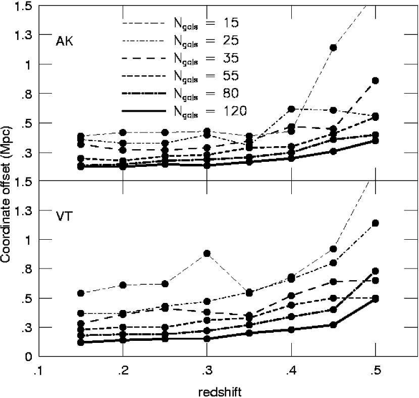
Figure 21: Positional offsets (in Mpc) for the VT and AK codes as a function of redshift. Each line represent a different richness class (N${}_{gals}=15,25,35,55,80,120$), with the thickest representing the richest clusters.

Figure 21 shows (for both the AK & VT) the positional offset (in Mpc) according to redshift for different richness classes. Each line represents a different richness class. Thicker lines represent richer clusters. For the poorer clusters the offset goes to infinity for higher redshifts ($z>0.40$). This simply means the recovery rate goes to zero for these clusters. We note that the offset is slightly larger and noisier for the VT code as compared to the AK. This is due to the percolation analysis needed for the VT, where we begin with candidates in different magnitude bins. An artificial cluster can have its recovered position slightly changed if it percolates with a nearby fluctuation.

We have also tried to evaluate the SF with four different matching radii for the VT code: 0.4, 0.75, 1.0 and 1.5 $h^{-1}$ Mpc. There is a great improvement when we go from 0.4 $h^{-1}$ Mpc to 0.75 $h^{-1}$ Mpc, while the SF does not change significantly for larger matching radii. Our final choice is 0.75 $h^{-1}$ Mpc for comparing the original positions of artificial clusters with the output of both our algorithms.

Finally, it is important to stress that the simulations used to assess the contamination rate (§4) only provide a lower limit. Similarly, the cluster simulations employed provide only an upper limit for the completeness rate of the catalog.

7 Performance comparison of the two algorithms

The AK cluster catalog contains 4,813 candidates, whereas the VT contains 7,962. The combined catalog shown in Figure 17 contains 9,956 cluster candidates. Based on Figures 11 and 20, we expect the AK catalog to have more rich clusters, and to go deeper, compared to the VT catalog. On the other hand, the VT catalog is more complete in the regime of poor/nearby systems. The redshift and richness distributions of the cluster candidates confirm the expectations from the simulations. The cutoffs in every panel of Figures 14 and 15 show that the cluster distributions are in good agreement with the SFs.

We stress that both methods applied here are simple density estimators, which detect fluctuations in the projected galaxy distribution above a given threshold. Both methods make no assumptions whatsoever on any physical properties of galaxy clusters (e.g., the luminosity function, colors of galaxy members, spatial profile, etc). The AK code is sensitive to an initial smoothing scale, while the VT does not distribute the data in bins. However, with the proper choice of the initial kernel size, we expect the AK to be as sensitive to irregular structures as the VT. We believe the differences shown here arise from the way we minimize the background in each case. The VT is applied to galaxies spanning a wide range of magnitudes (16.0 $\leq m_{r}\leq 21.1$), while the AK code is applied only to the faint data of DPOSS (the bright cut is at $m_{r}=19.0$). Thus, the AK naturally avoids nearby fluctuations and enhances the contrast of distant systems, while we employ a binning scheme to minimize contamination for the VT algorithm. Obviously, these same density estimators when applied to multi-wavelength data provide a much more powerful tool to minimize background/foreground contamination (Kim et al., 2002; Goto et al., 2002; Gladders & Yee, 2000).

The comparison of catalogs generated by these different techniques is not a straightforward task. As noted by Kim (2001), clusters are missed by one method and not by another due to the fact that they are seen with different eyes. Some cluster finding techniques will be biased to clusters with some specific properties, thus having a low efficiency for overdensities that do not match these properties. Furthermore, clusters which are recovered by various techniques might have large differences in the measurement of properties such as richness, redshift and projected density profile.

Kim (2001) used a 0.7 h^-1 Mpc radius when matching candidates from different algorithms. However, she finds that, in some cases, the cluster centers from different algorithms can differ by as much as the extent of the cluster. This could be especially true for poor and irregular clusters. Large differences in the redshift estimates for candidates from the two codes would make this comparison more difficult, or even impossible. However, we do not expect the photometric redshifts to have a large variation in our case. So, we decided to adopt a physical radius, instead of an apparent radius when comparing the AK and VT catalogs. We use a 0.75 h^-1 Mpc maximum radius, as done for the evaluation of the selection functions.

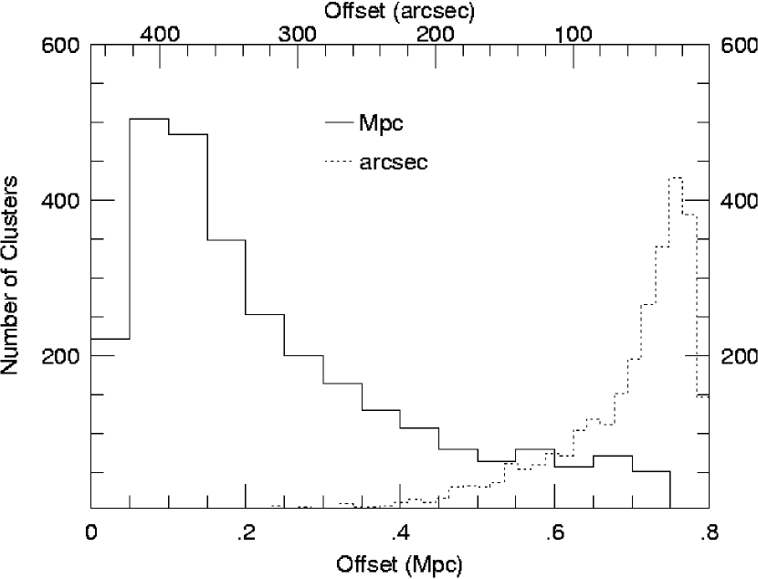
Figure 22: Centroid offset distribution for common clusters from the VT and AK codes. Offsets in Mpc are indicated by the solid line, while the offsets in arcsec are represented by the dotted line.

Out of the 4,813 (AK) and 7,962 (VT) cluster candidates, 2819 (59% of AK and 35% of the VT) are common sources. The VT catalog is denser than the AK catalog because it is more complete in the regime of poor systems, which are more abundant. Figure 22 shows the offset distribution for the matched clusters in Mpc (solid line) and arcseconds (dotted line). Most clusters show no large offsets (less than 100^′′ or 0.40 h^-1 Mpc). The combined catalog is presented in Table 1 and Figure 17.

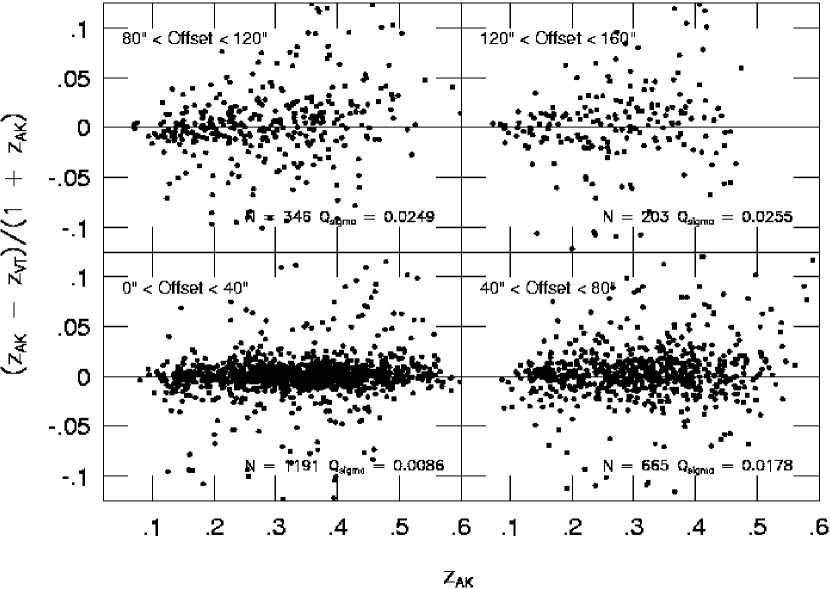
Figure 23: The dependence of the redshift estimate on the cluster centroid. Redshift residuals as a function of redshift are shown for different offset ranges, which are indicated on each panel. The number of clusters (N) is also indicated.

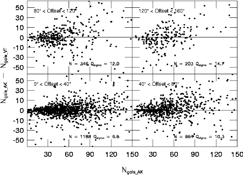
Figure 24: Richness residuals as a function of richness are shown for different offset ranges, which are indicated on each panel. The number of clusters (N) is also indicated.

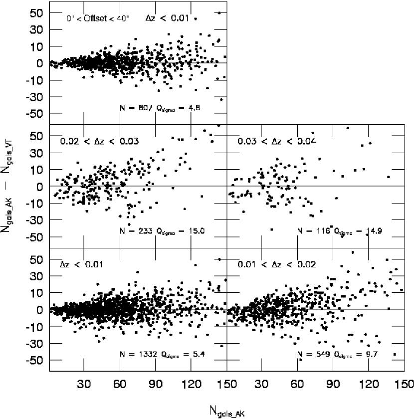
Figure 25: Richness residuals as a function of richness are shown for different bins of redshift residuals (indicated on each panel). The number of clusters (N) is also indicated. The upper left panel shows the results when selecting only clusters with offsets $<40^{\prime\prime}$ and $\Delta z<0.01$.

Redshift and richness estimates are obtained post-detection. They are, however, sensitive to the cluster center, as the corrected cluster galaxy counts will depend on this choice. We then divide the common clusters into bins of 40^′′ in centroid offsets, from 0^′′ to 160^′′. The residuals as a function of redshift for different offsets are shown in Figure 23, with a clear trend to large residuals for large offsets. Figure 24 shows the same effect, but for richness. Finally, we investigate the dependence of the richness measurement on the adopted redshift. Figure 25 is similar to the previous one, but the bins are in redshift residuals (from $\Delta z=0.01$ to 0.04, in steps of 0.01), instead of cluster center offsets. The top left panel shows the results when cutting the sample at offset $<40^{\prime\prime}$ and $\Delta z<0.01$. There is an evident improvement when comparing this panel to the bottom left panels of this Figure and Figure 24.

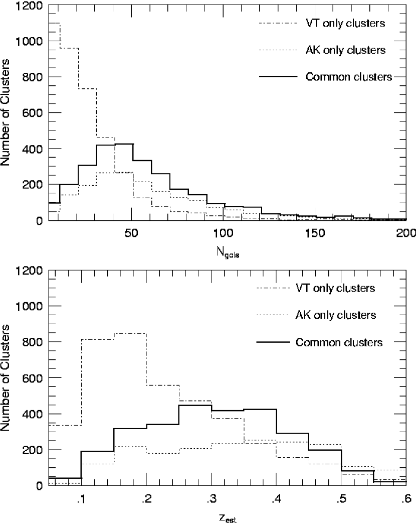
Figure 26: Richness (top) and estimated redshift (bottom) distributions for clusters detected only by the VT code (dashed-dotted line), only by the AK code (dotted line) and by both methods (heavy solid line).

We show in Figure 26 richness (top) and redshift (bottom) distributions for VT only detections (dashed-dotted line), AK only clusters (dotted line) and common candidates (heavy solid line). This plot fully confirms the expectations from the selection function estimates. We expect the VT code to perform better for poor, nearby clusters, while the AK should go deeper when detecting rich systems. This is clearly seen in Figure 26, where most of the VT-only detections are nearby poor systems, while the AK-only clusters are mainly distant and rich. The two catalogs overlap at intermediate richnesses and redshifts.

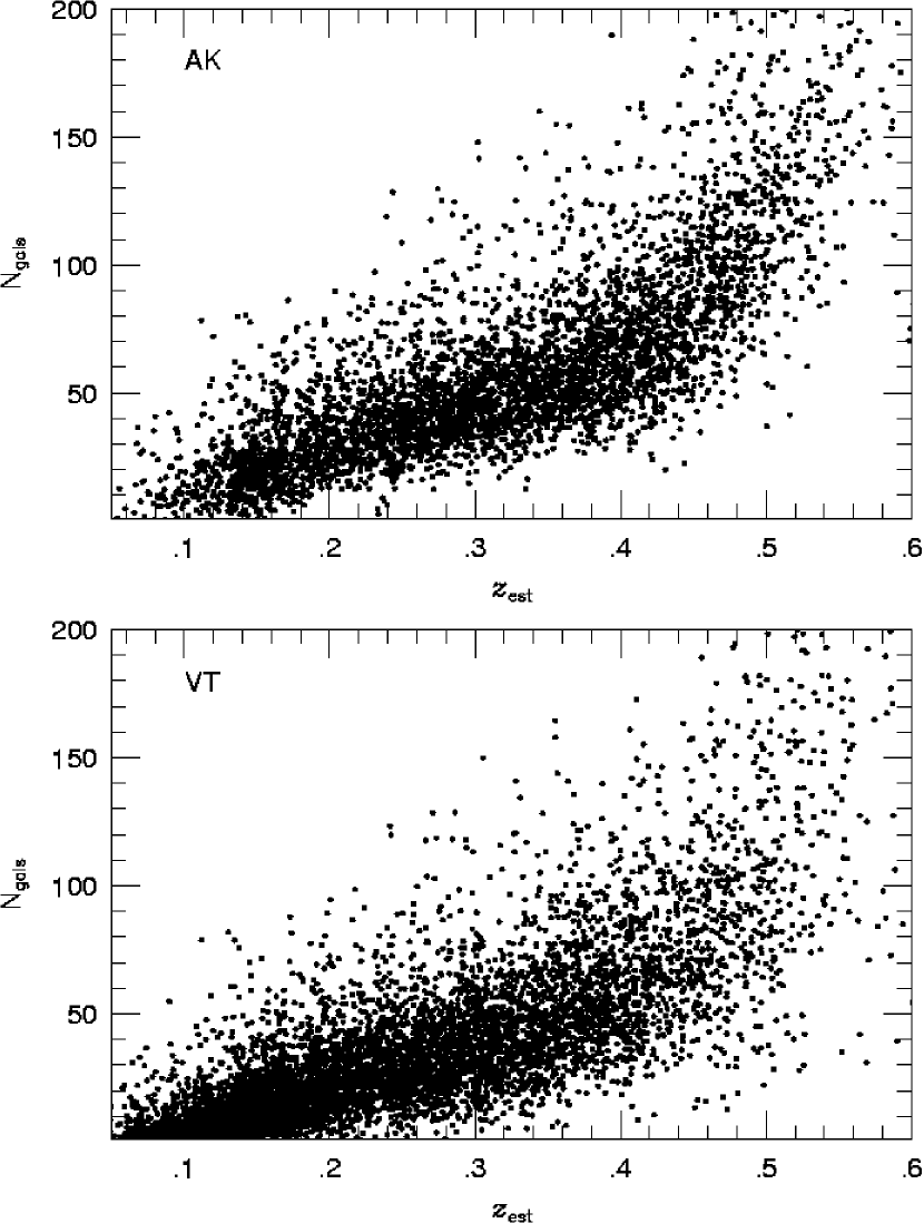
Figure 27: Richness vs. estimated redshift for the AK (top) and VT (bottom) candidates.

Figure 27 shows the distribution of N_gals with respect to the estimated redshift for both the AK and VT. A similar dependence was previously found by Kim (2001). The richer systems are rarely found at low redshifts where we probe less physical volume per unit redshift interval. On the other hand, the poor clusters are easier to detect at low redshift, where they are still seen as high-contrast systems. One surprising result is that only the VT code apparently finds relatively poor systems (N${}_{gals}\lesssim 60$) at $z>0.45$. For these faint systems the redshift and richness estimates are more difficult to measure as the number of galaxies used for these estimates is typically low. The VT code is also less accurate than the AK algorithm in determining the centroid of a cluster (Figure 21). For these low contrast systems, this can have a great impact to the redshift and richness estimates, and could result in underestimation of the richness. Note also that Kim (2001) found the same trend for the VT candidates when using SDSS data.

Finally, we test the overlap of both catalogs in the regime where they are expected to have high completeness. The SF predicts that both cluster catalogs are nearly complete for rich clusters (N${}_{gals}\gtrsim 65$) at $0.2<z<0.3$ (Figures 11 and 20). To be conservative we assume a completeness level $>90\%$, and select all cluster candidates from both catalogs for these richness classes in this redshift range. We find 87 VT and 108 AK candidates. Out of the 87 VT candidates, 84 have a match in the AK catalog, which represents an overlap of $\sim 78\%$, in agreement with the expectations from the SF.

8 Comparison with other cluster surveys

A comparison of the NoSOCS and the Abell cluster catalogs was previously done in Papers II and III. We would like to compare the supplemental NoSOCS catalog presented here to other intermediate redshift cluster catalogs. The best sources of comparison are given by the preliminary SDSS catalogs (Kim, 2001; Goto et al., 2002), which are used as a reference for the comparison shown in the end of this section. Additionally, as the DPOSS data used differs from that used in Papers II and III, we also perform comparisons with those catalogs. We also investigate differences in the redshift and richness measurements. As stated before, there are some fundamental differences in the estimates presented here and in the previous DPOSS papers.

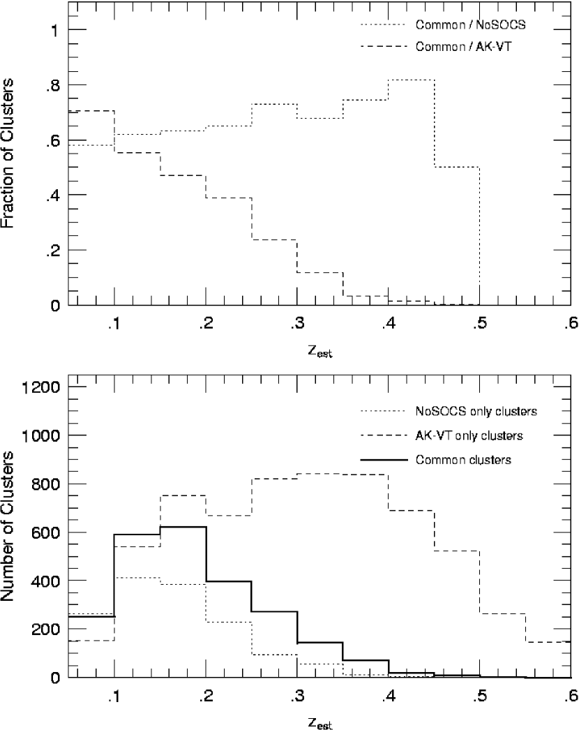
Figure 28: Estimated redshift distributions (bottom panel) for clusters detected only in Papers II & III (dotted line), only by this paper (dashed line) and by both surveys (heavy solid line). The top panel shows the ratio of common clusters to the NoSOCS catalog (dotted line) and to the supplemental catalog presented here (dashed line).

From the $>$ 12,000 NoSOCS (Papers II and III) cluster candidates over the entire high latitude ($|b|>30^{\circ}$) northern sky, we find 4,211 candidates within the 2,700 square degrees sampled here. As done before, we adopt a 0.75 h^-1 Mpc radius when comparing two catalogs. We find 2,638 clusters common to both catalogs. Figure 28 shows the estimated redshift distribution (bottom panel) of NoSOCS only clusters (Papers II and III) as dotted lines, while the dashed lines represents the distribution of clusters present only in the current survey. The distribution of common clusters is represented by the heavy solid line. It is clear that most new candidates found here have $z_{est}\gtrsim 0.2$. In the top panel of the same Figure we show the ratio of common clusters to each of the catalogs. The dotted line represents the ratio to the catalog from Papers II and III, while the dashed line is the ratio of common clusters to the supplemental catalog presented here. Out to $z_{est}\sim 0.2$, approximately 60% of NoSOCS clusters are common to the new catalog, with almost all of the common detections at low-$z$.

It is important to stress that poor clusters at $z<0.2$ detected in Papers II & III might not be easily recovered using the methods presented here. The AK catalog is obviously biased against these systems due to the bright magnitude cut ($m_{r}\sim 19$), while the VT code might have problems recovering these nearby, low contrast structures. The binning scheme adopted to enhance the cluster contrast might not be powerful enough to enable recovery of these systems. Note also that the matching radius employed when comparing the two catalogs is crucial to the analysis. Poor systems might have large differences in the centroid determination, especially if the centroid is given by galaxies in different magnitude ranges. Goto et al. (2002) adopted a 6^′ radius to compare their catalog to other SDSS cluster catalogs. We preferred to adopt a physical radius of 0.75 h^-1 Mpc to compare any two catalogs, even considering possible discrepancies in the photo-z estimates. In the regime where they are expected to have high completeness ($0.1<z<0.2$ and N${}_{gals}\gtrsim 65$), the cluster catalog from Papers II and III has 38 rich clusters. The VT catalog finds 33 of those, while the AK catalog finds 27. The mean overlap is $\sim$ 79%. For the few missing clusters we pointed the richness estimator code to the coordinates given in Papers II & III, also adopting the redshift estimate given there. We found these systems to be poor clusters in the deeper galaxy catalog used here. In other words, the contrast of these clusters decreases when seen in a wider magnitude range.

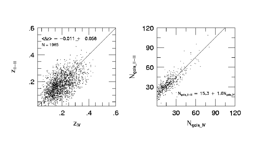
Figure 29: Comparison between our catalog and those from Papers II and III. On both panels the abscissa has the results for the current paper (IV), while the ordinate shows the results from Papers II and III. The left panel shows the redshift estimates for 1,985 common clusters between this paper and the previous two. On the right richness estimates for $z<0.2$ clusters are compared.

In Figure 29 we plot the NoSOCS photometric redshift estimates (Gal et al., 2003) against those from this paper (left panel). If we assume the estimates from Papers II & III are more correct than those presented here, then we have some indication that our redshifts are overestimated. In the right panel we compare the richness estimates for nearby clusters ($z<0.2$). As stated in section 5.2, there are many differences between the richness estimates presented here and in the previous DPOSS papers. First, the galaxy catalogs are deeper and have a statistical correction applied to them, which could affect the cluster contrast. Second, we now adopt a local background correction, while the background counts were previously taken from a plate scale (Papers II & III). In the previous papers, the $\gamma$ correction factor considered all galaxies to be elliptical, while here we consider only 60% to be ellipticals.

Finally we compare our catalog to the SDSS cluster catalogs presented in Kim (2001) and Goto et al. (2002). Both catalogs cover an equatorial strip of $\sim 350\square^{\circ}$. However, most of the common clusters (between SDSS and DPOSS) are found in the RA $\lesssim 44^{\circ}$ region, as we have only two plates in the North Galactic Pole region which are also in this equatorial strip. The coordinate limits used to trim both SDSS catalogs, as well as ours, are $-2.1^{\circ}\leq\alpha\leq 43.75^{\circ},-1.27^{\circ}\leq\delta\leq+1.27^{\circ}$. There are 863 clusters from Kim (2001), 1288 from Goto et al. (2002) and 471 AK-VT candidates in this region. The catalog from Kim (2001) is the combination of two catalogs, using a Hybrid Matched Filter and a Voronoi Tessellation technique, and is hereafter called HMF-VT.

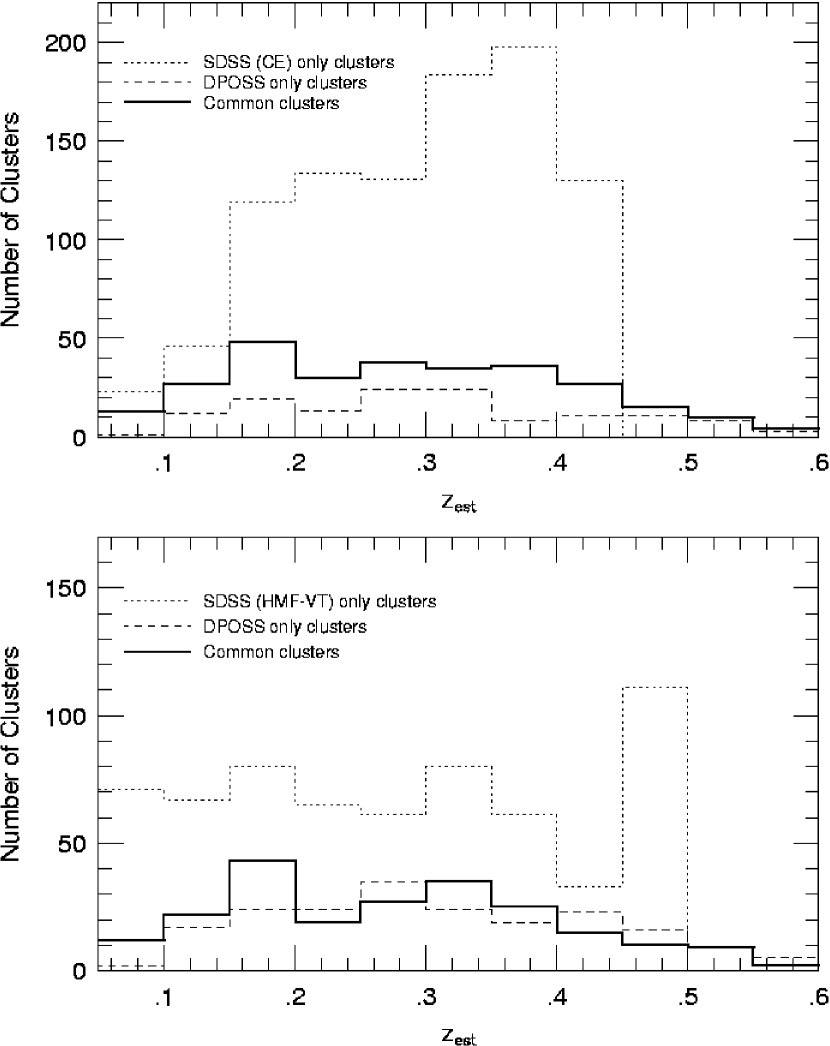
Figure 30: Estimated redshift distributions of DPOSS only clusters (dashed lines), common clusters (heavy solid line) and SDSS only clusters (dotted line). In the bottom panel DPOSS is compared to the catalog presented in Kim (2001), while the comparison to the CE catalog (Goto et al., 2002) is shown in the top panel.

In Figure 30 we show the estimated redshift distributions of clusters detected only by DPOSS (dashed line), common clusters (heavy solid line), and SDSS only clusters (dotted lines). In the top panel the DPOSS cluster catalog is compared to the SDSS Cut & Enhance (CE) catalog (Goto et al., 2002), while in the bottom panel the comparison is made to the catalog of Kim (2001). In both panels the unmatched detections have redshift estimates from their own detection method, while matched clusters have our redshift estimates. The HMF-VT catalog (Kim, 2001) recovers many more nearby (probably poor) clusters than DPOSS, while the CE catalog (Goto et al., 2002) goes deeper than DPOSS. This result also points to intrinsic differences in the clusters sampled by the two SDSS catalogs.

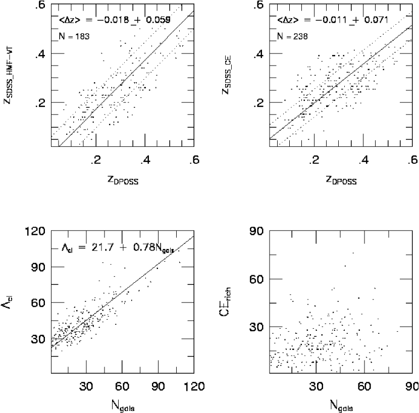
Figure 31: Comparison between our catalog and those from Kim (2001) & Goto et al. (2002). In the top panels we compare our redshift estimates to those from Kim (2001) (left) and Goto et al. (2002) (right). The solid lines represent the best fit, while the dashed lines give the combined $rms$ from the two catalogs, on each panel. The bottom panels show the richness comparisons.

In the top panels of Figure 31, our redshift measurements are compared to those from both SDSS catalogs. The estimates of Kim (2001) have an rms comparable to ours, while Goto et al. (2002) measurements are much more precise ($\Delta z<0.02$). Despite the offset, we find a better agreement when comparing our estimates to those from Kim (2001) than those from Goto et al. (2002). This might be due to the fact that Kim’s estimates use magnitude information (as we do), while the CE estimates are based only on the $g-r$ color (which limits high-$z$ estimates due to the shift of the 4000Å  break to the $r-i$ color).

When comparing richness measurements we re-measure N_gals for the common clusters, using the coordinates and redshift estimates provided in the SDSS catalogs. This procedure minimizes the effects seen in Figures 23 to 25. The richness measure given by Kim (2001) is called $\Lambda_{cl}$, which represents the total cluster luminosity within 1.0 $h^{-1}$ Mpc in units of $L^{*}$. N_gals also considers a 1 $h^{-1}$ Mpc counting radius, but we only sample galaxies at $M^{*}-1\leq M\leq M^{*}-2$. Goto et al. (2002) count galaxies from $m_{3}$ to $m_{3}+2$ (where $m_{3}$ is the third brightest cluster galaxy) within the detection radius provided by the CE algorithm. As they state, this is similar to the Abell richness, except for the counting radius, which is chosen differently for the CE method. The bottom left panel of Figure 31 shows the relation between $\Lambda_{cl}$ and N_gals. As we adopt the same coordinates and $z_{est}$ provided by Kim (2001), we expect the scatter to originate mainly from the differences in the galaxy catalogs used for the richness estimation. Considering the higher quality of the SDSS data compared to the DPOSS plate data, the small scatter shown in this plot is an encouraging result. The bottom right panel shows the comparison between the CE richness and N_gals. The scatter is extremely large and no obvious relation is found. We believe this is unrelated to the nature of the data, but mainly to the choice of an apparent radius to count galaxies for the CE richness. Even a direct comparison between the two SDSS richnesses, $\Lambda_{cl}$ and that from the CE, is difficult.

The cluster number density presented here is over 2 times greater than that found in Papers II and III. This is sensible as we sample many more distant clusters when compared to our previous papers. The more interesting comparison, however, is to the SDSS catalogs. The Gunn $r$-band has a similar response to the SDSS $r^{*}$ filter, which renders our $m_{r}=21.1$ limit similar to that adopted by Kim (2001) and a little brighter than the choice of Goto et al. (2002). Thus, the cluster catalogs’ depths should be similar. The cluster catalogs will differ due to the quality of the data used, the detection algorithms, and the contamination level allowed.

The number density of the HMF clusters is 7.8 clusters per square degree (Kim, 2001), 13.3 for the CE catalog (Goto et al., 2002), and 3.7 for our catalog. The main reasons that the HMF-VT catalog finds over twice as many clusters as our technique are the higher quality photometric data of SDSS and the higher contamination rate allowed by Kim (2001) (15% compared to our 5%). The CE catalog has an extremely high number density. This is likely due to their fainter magnitude limit, and their high ($\sim 30\%$) contamination rate in the regime of poor clusters (where most candidates are). The CE method is a powerful technique to detect clusters and minimize background/foreground contamination, but the very high number density of supposedly real clusters may not be justified. A closer examination of our redshift distribution (Figure 14) when compared to Figure 26 of Goto et al. (2002) reveals that in the regime of rich clusters our catalog goes as deep as all the SDSS catalogs. However, the HMF-VT method samples many more poor/nearby systems than our technique, while the CE catalog detects many more high-redshift candidates ($z_{est}>0.25$). Nonetheless, it seems that the SFs presented in Goto et al. (2002) may not be in good agreement with their redshift distribution. They appear to actually go deeper than indicated by the SFs.

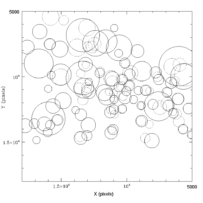
Figure 32: The sky distribution of candidates detected in the central region of DPOSS Field 824 ($\alpha=5.65^{\circ},~{}\delta=0.26^{\circ}$). AK-VT candidates are indicated by dashed circles and the HMF-VT clusters by solid circles. We adopt a 1.5 $h^{-1}$ Mpc radius for this illustration. When the redshift estimator code fails we adopt $z=0.3$ to draw the circle.

An illustration of the higher density of the SDSS HMF-VT catalog compared to this AK-VT catalog is given in Figure 32. We show the candidate distribution for the central region of DPOSS field 824. HMF-VT candidates are shown as solid circles, while the AK-VT candidates are plotted with dashed circles. The circles represent a 1.5 $h^{-1}$ Mpc radius at the estimated redshift. Two features are readily noticed. First, the HMF-VT only clusters are generally low-$z$ systems as indicated by the large radii of the candidates missed in our survey. Second, the HMF-VT is able to recover cluster candidates at different redshifts along the same line of sight, while our method cannot distinguish between these superposed systems. In most such cases, we recover the fainter, more distant clusters instead of the closer ones.

Finally, as done in the comparison to the catalogs presented in Papers II & III, we test for disagreements with the SDSS catalogs where SDSS and DPOSS predict high completeness levels. Using the relation between $\Lambda_{cl}$ and N_gals, we convert the HMF-VT richness estimates to N_gals. We look for clusters with N${}_{gals}>65$ at $0.2<z_{est}<0.3$. There are only 2 clusters in this regime in the HMF-VT catalog and 6 in our catalog. Both clusters found by Kim (2001) have a match in our catalog, while 3 of the 6 AK-VT candidates have a match in the HMF-VT list. As we can not convert the CE richness estimate to N_gals we simply chose a richness cut for the CE catalog. We selected all clusters with CE${}_{rich}>40$ at $0.2<z_{est}<0.3$. Out of 18 CE clusters in this regime, 11 have a counterpart in our catalog. We would like to stress that centroid and redshift estimates discrepancies, as well as the non-negligible scatter in the $\Lambda_{cl}-$N_gals relation, render this comparison problematic. Note also that the CE_rich cut ($>40$) has no relation to N${}_{gals}>65$, so the comparison between CE and AK-VT has no correspondence to the comparison between the HMF-VT and AK-VT catalogs.

9 Summary

This paper presents an intermediate redshift galaxy cluster catalog ($0.1\lesssim z_{est}\lesssim 0.5$) covering 2,708 $\square^{\circ}$ of DPOSS data, providing a supplement to those presented in papers II and III. The catalog is the result of two different density estimators (AK & VT) and its combined version contains $\sim$ 10,000 cluster candidates. To facilitate the selection of subsamples for follow-up studies we provide both redshift and richness estimates. The redshift estimates are as accurate as the matched filter redshift output. By keeping the contamination rate at 5%, the probability of selecting false clusters is minimized. Our catalog is cleaned post-detection, to discard obvious false candidates due to bright stars, nearby galaxies and groups, etc.

The main goal of this project is to provide a catalog of rich clusters to $z_{est}\sim 0.5$ covering a large area of the Northern sky. It is a valuable source for follow-up studies, which can be used to select candidates for lensing studies, to study the cluster population at intermediate redshifts, to search for optical rich clusters with low X-ray luminosity, etc. We plan to carry out a spectroscopic survey of a subsample of this catalog to confirm the reality of these systems, as well as deep imaging follow-up.

We present a detailed comparison of the results obtained by the different algorithms, showing the dependence of the redshift and richness estimates on cluster centroid, as well as the richness variation associated to the redshift estimate. We also find a high level of overlap in the regime where both catalogs are expected to have high completeness.

Our catalog is also compared to other recent surveys, showing excellent agreement with those where all catalogs are expected to have high completeness rates (rich clusters at $0.2<z_{est}<0.3$). However, the cluster catalogs derived from the higher quality multi-color data of SDSS are more complete than our catalog. The HMF-VT detects more poor/nearby systems, while the CE catalog is more complete for higher-$z$ systems. Nonetheless, this work provides the largest resource for galaxy clusters spanning this redshift range to date. It will certainly be superseded in the near future by the whole sky catalogs generated from SDSS. However, it represents the first effort to search for clusters out to the faintest limits of a sky survey over such a large area. This cluster catalog also constitutes an excellent resource for comparison with the final SDSS catalog, as well as to deep X-ray cluster catalogs.

Figure 20: Comparison of the selection function evaluated with three different cluster compositions. The top panel shows the results for 20% E & 80% Sbc, the middle panel is for 60% E & 40% Sbc, while the bottom panel is for 100% ellipticals. The richness classes are as indicated in Figure 11.

Table 1: The Northern Sky Cluster Catalog Supplemental: Excerpt

Name	RA (J2000.0)	Dec (J2000.0)	$z_{phot-AK}$	$z_{phot-VT}$	$N_{gals-AK}$	$N_{gals-VT}$	Plate	codes
NSCS J133609+292956	204.035858	29.498718	0.48	0.49	126.7	130.2	444	AV
NSCS J132532+314613	201.384430	31.770241	0.44	0.45	67.2	67.7	444	AV
NSCS J132421+310806	201.085632	31.134737	0.42	0.42	88.2	76.3	444	AV
NSCS J132350+304404	200.959229	30.734278	0.46	0.49	128.8	158.0	444	AV
NSCS J132049+320530	200.205231	32.091518	0.47	0.00	75.5	0.0	444	A
NSCS J131747+315539	199.446884	31.927435	0.44	0.00	63.0	0.0	444	A
NSCS J132036+314133	200.149994	31.692387	0.49	0.00	79.8	0.0	444	A
NSCS J131644+312003	199.183975	31.334074	0.40	0.40	74.6	66.3	444	AV
NSCS J133557+304355	203.987961	30.731905	0.42	0.42	81.3	76.7	444	AV
NSCS J132303+303959	200.764053	30.666296	0.47	0.44	97.3	58.4	444	AV
NSCS J132405+303250	201.019501	30.546940	0.43	0.44	70.4	71.5	444	AV
NSCS J132336+302223	200.898285	30.373018	0.48	0.49	97.6	92.3	444	AV
NSCS J134222+280715	205.593262	28.120775	0.44	0.44	217.4	201.3	445	AV
NSCS J134316+282308	205.817719	28.385321	0.44	0.00	113.3	0.0	445	A
NSCS J135107+305444	207.779678	30.912178	0.45	0.43	151.2	118.3	445	AV
NSCS J140607+271029	211.527512	27.174681	0.49	0.50	120.5	131.5	446	AV*
NSCS J140457+272800	211.235489	27.466606	0.50	0.50	159.7	133.1	446	AV
NSCS J140612+282513	211.549500	28.420187	0.42	0.39	69.8	56.9	446	AV
NSCS J140436+283443	211.148712	28.578556	0.45	0.46	175.6	150.9	446	AV
NSCS J140614+282911	211.556107	28.486269	0.46	0.00	65.7	0.0	446	A
NSCS J140733+283829	211.887100	28.641354	0.43	0.43	66.1	71.4	446	AV
NSCS J141119+295227	212.827988	29.873974	0.46	0.00	134.0	0.0	446	A
NSCS J143630+290031	219.126694	29.008404	0.49	0.42	132.4	83.3	447	AV
NSCS J144045+292800	220.186127	29.466623	0.44	0.44	173.9	163.4	447	AV
NSCS J143307+294227	218.279083	29.707354	0.41	0.42	91.5	97.2	447	AV
NSCS J144332+315050	220.881851	31.847206	0.42	0.42	74.2	64.9	447	AV
NSCS J142727+304153	216.864319	30.697830	0.47	0.00	126.6	0.0	447	A
NSCS J150804+280926	227.017517	28.157183	0.48	0.00	167.3	0.0	448	A
NSCS J145024+322408	222.598465	32.402100	0.44	0.00	99.6	0.0	448	A *
NSCS J144940+321048	222.414612	32.179859	0.45	0.45	155.1	156.9	448	AV
NSCS J150449+321740	226.201996	32.294426	0.45	0.00	109.6	0.0	448	A
NSCS J150143+321237	225.430496	32.210087	0.45	0.00	176.5	0.0	448	A
NSCS J145329+321024	223.369202	32.173214	0.45	0.50	134.0	198.4	448	AV
NSCS J144802+320520	222.008209	32.088737	0.46	0.00	234.8	0.0	448	A
NSCS J151043+320608	227.677841	32.102161	0.48	0.00	271.5	0.0	448	A

References

- Abell (1958) Abell, G. O. 1958, ApJS, 3, 211
- Abell, Corwin & Olowin (1989) Abell, G. O., Corwin, H. G. & Olowin, R. P. 1989, ApJS, 70, 1
- Annis et al. (1999) Annis, J. et al. 1999, BAAS, 195
- Aragón-Salamanca et al. (1993) Aragón-Salamanca, A., Ellis, R., Couch, W., Carter, D. 1993, MNRAS, 262, 764
- Bahcall & Soneira (1983) Bahcall, N. A. & Soneira, R. M. 1983, ApJ, 270, 20
- Bahcall et al. (1997) Bahcall, N. A., Fan, X., Cen, R. 1997, ApJ, 485, L53
- Bahcall et al. (2003) Bahcall, N. A. et al. 2003, ApJS, 148, 243
- Bertin & Arnouts (1996) Bertin, E. & Arnouts, S. 1996, A&AS, 117, 393
- Böhringer et al. (2000) Böhringer, H. et al. 2000, ApJS, 129, 435
- Bramel, Nichol & Pope (2000) Bramel, D. A., Nichol, R. C. & Pope, A. C. 2000, ApJ, 533, 601
- Butcher & Oemler (1984) Butcher, H. & Oemler, A. 1984, ApJ, 285, 426
- Carlberg et al. (1996) Carlberg, R., Yee, H., Ellingson, E., Abraham, R., Gravel, P., Morris, S., Pritchet, C. 1996, ApJ, 462, 32
- Carlberg et al. (1997) Carlberg, R., Morris, S., Yee, H., Ellingson, E. 1997, ApJ, 479, L19
- Coleman, Wu, & Weedman (1980) Coleman, G. D., Wu, C. C., & Weedman, D. W. 1980, ApJS, 43, 393
- Dalton, Maddox, Sutherland & Efstathiou (1997) Dalton, G. B., Maddox, S. J., Sutherland, W. J. & Efstathiou, G. 1997, MNRAS, 289, 263
- Djorgovski et al. (2004) Djorgovski, S. G., Gal, R. R., de Carvalho, R. R., Odewahn, S. C., Mahabal, A., Brunner, R. J. & Lopes, P. 2004, AJ, in prep.
- Doroshkevich et al. (1997) Doroshkevich, A., Gottlober, S., Madsen, S. 1997, A&AS, 123, 495
- Dressler et al. (1997) Dressler, A., Oemler, A., Couch, W., Smail, I., et al. 1997, ApJ, 490, 577
- Ebeling & Wiedenmann (1993) Ebeling, H., Wiedenmann, G. 1993, Phys. Rev. E, 47, 704
- El-Ad et al. (1996) El-Ad, H., Piran, T. da Costa, L. 1996, ApJ, 462, 13
- Evrard (1989) Evrard, A. 1989, ApJ, 341, L71
- Gal et al. (2000) Gal, R. R., de Carvalho, R. R., Odewahn, S. C., Djorgovski, S. G. & Margoniner, V. E. 2000, AJ, 119, 12
- Gal et al. (2003) Gal, R. R., de Carvalho, Lopes, P. A. A., Djorgovski, S. G., Brunner, R. J., Mahabal, A., Odewahn, S. C. 2003, AJ, 125, 2064
- Gal et al. (2004a) Gal, R. R., de Carvalho, R. R., Odewahn, S. C., Djorgovski, S. G., Mahabal, A., Brunner, R. J., Lopes, P. 2004a, AJ, accepted
- Gal et al. (2004b) Gal, R. R., de Carvalho, Lopes, P. A. A., Djorgovski, S. G., Brunner, R. J., Mahabal, A., Odewahn, S. C. 2004b, AJ, in prep.
- Gilbank (2001) Gilbank, D. 2001, Ph.D. Thesis, University of Durham
- Gladders & Yee (2000) Gladders, M. D. & Yee, H. K. C. 2000, AJ, 120, 2148
- Gonzalez, Zaritsky, Dalcanton, & Nelson (2001) Gonzalez, A. H., Zaritsky, D., Dalcanton, J. J., & Nelson, A. 2001, ApJS, 137, 117
- Goto et al. (2002) Goto, T. et al. 2002, AJ, 123, 1807
- Gunn, Hoessel & Oke (1986) Gunn, J. E., Hoessel, J. G. & Oke, J. B. 1986, ApJ, 306, 30
- Guzzo et al. (1992) Guzzo, L., Collins, C., Nichol, R., Lumsden, S. 1992, ApJ, 393, 5
- Hg et al. (2000) Hg, E., Fabricius, C., Makarov, V., Urban, S., Corbin, T., Wycoff, G., Bastian, U., Schwekendiek, P., Wicenec, A. 2000, A&A, 355, 27
- Holden et al. (1999) Holden, B., Nichol, R., Romer, A., Metevier, A., Postman, M., Ulmer, M., Lubin, L. 1999, AJ, 118, 2002
- Ikeuchi & Turner (1991) Ikeuchi, S. & Turner, E. 1991, MNRAS, 250, 519
- Kawasaki et al. (1998) Kawasaki, W., Shimasaku, K., Doi, M., Okamura, S. 1998, A&AS, 130, 567
- Kepner et al. (1999) Kepner, J., Fan, X., Bahcall, N., Gunn, J., Lupton, R. & Xu, G. 1999, ApJ, 517, 78
- Kiang (1996) Kiang, T. 1996, Zeitschrift für Astrophysik, 64, 433
- Kim (2001) Kim, R. S. J. 2001, Ph.D. Thesis, Princeton
- Kim et al. (2002) Kim, R. S. J. et al. 2002, AJ, 123, 20
- Lobo et al. (2000) Lobo, C., Iovino, A., Lazzati, D. & Chincarini, G. 2000, A&A, 360, 896
- Lumsden, Nichol, Collins & Guzzo (1992) Lumsden, S. L., Nichol, R. C., Collins, C. A. & Guzzo, L. 1992, MNRAS, 258, 1
- Maddox, Efstathiou & Sutherland (1996) Maddox, S. J., Efstathiou, G. & Sutherland, W. J. 1996, MNRAS, 283, 1227
- Margoniner et al. (2001) Margoniner, V. E., de Carvalho, R. R., Gal, R. R., Djorgovski, S. G. 2001, ApJ, 548, L143
- Mullis et al. (2003) Mullis, C., McNamara, B., Quintana, H., Vikhlinin, A., Henry, J., Gioia, I., Hornstrup, A., Forman, W., Jones, C. 2003, ApJ, 594, 154
- Odewahn et al. (2004) Odewahn, S. C., Gal, R. R., de Carvalho, R. R., Djorgovski, S. G., Mahabal, A., Brunner, R. J., Lopes, P. A. A., Kohl Moreira, J. L., Stalder, B. 2004, AJ, submitted
- Olsen et al. (1999) Olsen, L. F. et al. 1999, A&A, 345, 363
- Paolillo et al. (2001) Paolillo, M., Andreon, S., Longo, G., Puddu, E., Gal, R. R., Scaramella, R., Djorgovski, S. G., & de Carvalho, R. 2001, A&A, 367, 59
- Picard (1991) Picard, A. 1991, Ph.D. Thesis, Caltech
- Postman, Huchra & Geller (1992) Postman, M., Huchra, J., & Geller, M. 1992, ApJ, 384, 404
- Postman et al. (1996) Postman, M., Lubin, L. M., Gunn, J. E., Oke, J. B., Hoessel, J. G., Schneider, D. P. & Christensen, J. A. 1996, AJ, 111, 615
- Postman et al. (1998) Postman, M., Lauer, T., Szapudi, I., Oegerle, W. 1998, ApJ, 506, 33
- Postman, Lauer, Oegerle, & Donahue (2002) Postman, M., Lauer, T. R., Oegerle, W., & Donahue, M. 2002, ApJ, 579, 93
- Ramella et al. (2001) Ramella, M., Boschin, W., Fadda, D., Nonino, M. 2001, A&A, 368, 776
- Reid et al. (1991) Reid, I. N. et al. 1991, PASP, 103, 661
- Schuecker & Böhringer (1998) Schuecker, P., Bhringer, H. 1998, A&A, 339, 315
- Shectman (1985) Shectman, S. A. 1985, ApJS, 57, 77
- Shewchuk (1996) Shewchuk, J. 1996, in First Workshop on Applied Comptutational Geometry, ACM
- Silverman (1986) Silverman, B. W. 1986, Monographs on Statistics and Applied Probability, London: Chapman and Hall
- Squires et al. (1996) Squires, G., Kaiser, N., Babul, A., Fahlman, G., Woods, D., Neumann, D. M., & Bhringer, H. 1996, ApJ, 461, 572
- Struble & Rood (1999) Struble, M. F. & Rood, H. J. 1999, ApJS, 125, 35
- Sunyaev & Zeldovich (1980) Sunyaev, R. A. & Zeldovich, Y. B. 1980, ARA&A, 18, 537
- Tyson & Fischer (1995) Tyson, J. A. & Fischer, P. 1995, ApJ, 446, L55
- Viana & Liddle (1996) Viana, P. T. P., Liddle, A. R. 1996, MNRAS, 281, 323
- Vikhlinin et al. (1998) Vikhlinin, A., McNamara, B, Forman, W., Jones, C., Quintana, H., Hornstrup, A. 1998, ApJ, 502, 558
- Wittman et al. (2001) Wittman, D., Tyson, J. A., Margoniner, V. E., Cohen, J. G., Dell’Antonio, I. P. 2001, ApJ, 557, 89
- Zaninetti (1995) Zaninetti, L. 1995, A&AS, 109, 71
- Zwicky, Herzog & Wild (1968) Zwicky, F., Herzog, E. & Wild, P. 1968, Catalogue of Galaxies and of Clusters of Galaxies, Pasadena: California Institute of Technology (CIT), 1961-1968