The multi-scale dust formation in substellar atmospheres

Abstract

Substellar atmospheres are observed to be irregularly variable for which the formation of dust clouds is the most promising candidate explanation. The atmospheric gas is convectively unstable and, last but not least, colliding convective cells are seen as cause for a turbulent fluid field. Since dust formation depends on the local properties of the fluid, turbulence influences the dust formation process and may even allow the dust formation in an initially dust-hostile gas.

A regime-wise investigation of dust forming substellar atmospheric situations reveals that the largest scales are determined by the interplay between gravitational settling and convective replenishment which results in a dust-stratified atmosphere. The regime of small scales is determined by the interaction of turbulent fluctuations. Resulting lane-like and curled dust distributions combine to larger and larger structures. We compile necessary criteria for a subgrid model in the frame of large scale simulations as result of our study on small scale turbulence in dust forming gases.

1 Introduction

The astrophysical field of substellar objects – of which brown dwarfs shall be considered as an example – has gained considerable attention during the last few years since more and more brown dwarfs and extrasolar planets could be detected. The need for appropriate models has increased with increasing observational resolution power which, however, can only provide information about the largest scale structures. The major challenge has been the observational evidence for the presence of dust (i.e. small solid or fluid particles) in substellar atmospheres where energy is mainly transported by convection. These gas parcels collide after their ascend through the atmosphere during which they adiabatically expand. Such adiabatic collisions cause turbulence, and the turbulent kinetic energy is transfered cascade-like from large to small scales. Due to its chemical nature, the dust formation process itself (like combustion) depends on local quantities like temperature, density and chemical composition of the gas, which can vary on much smaller spatial scale lengths than those accessible by observations. Photon interactions, molecular collisions and friction influence the dust formation process and proceed on scales comparable to or even less than one mean free path of the fluid, which belongs to the smallest relevant scale regime. The dust formation is hence initiated and controlled by small-scale processes, but produces consequences on the largest, observable scales.

The immediate couplings between chemistry, hydrodynamics and thermodynamics due to the presence of dust can cause an amplification of initially small perturbations resulting in the formation of large-scale dust clouds. The formation of such clouds is one of the major candidates to explain the observed non-periodic variability bm99; bm2001a; bm2001a; bm2001b; mzl2001; gm2002; clark2002 which is - from the physical point of view - very alike to what we know from weather-like variation in the Earth atmosphere. However, substellar object like brown dwarfs and known extraterrestrial planets show more extreme physical conditions (warmer and hotter or cooler and thinner) and the direct transfer of Earth’s knowledge has to be considered with care.

It was therefore the aim of this work to investigate the multi-scale problem of astrophysical dust formation in brown dwarf stars which requires an appropriate description of the chemical and turbulent processes and their interactions. The challenge in modeling turbulence in reactive gas flows lies in an adequate description of all relevant scale regimes. This work follows the scale hierarchy from the smallest to the largest scales. At first, turbulent dust formation will be studied on small scales (Sect. 3) which can be computationally resolved. These investigations intend to provide the basis for a sub-grid closure model for the next (larger) scale regime where it can be applied and so on. This procedure requires a detailed, scale-dependent view on the problem hlsk2001, or in other words, needs to adopt different windows of perception se2002.

2 The model of a dust forming gas flow

Redefining the variables of the system of model equations like $\alpha\rightarrow\alpha/\alpha_{\rm ref}$ transforms the equations in their scaled analogues wherein all quantities are dimensionless and can be compared by number. The non-dimensional characteristic numbers describe the importance of the source terms and general features can already be derived by investigating the dimensionless numbers for physical meaningful reference values.

Complex A: The specification of the source terms in the equations of momentum and energy conservation results in the following dimensionless system of equations which describe the fluid field in a substellar atmosphere which is influenced by the stellar radiation field holks2001b:

$$(\rho)_{t}+\nabla\cdot(\rho{\boldsymbol{v}}) = 0$$ (1)

$$Sr\,(\rho{\boldsymbol{v}})_{t}+\nabla\cdot(\rho{\boldsymbol{v}}\circ{\boldsymbol{v}}) = -\frac{1}{\gamma M^{2}}\nabla P-\frac{1}{Fr^{2}}\rho{\boldsymbol{g}}$$ (2)

$$(\rho e)_{t}+\nabla\cdot({\boldsymbol{v}}[\rho e+P]) = Rd_{1}\,\kappa(T^{4}_{\rm RE}-T^{4}),$$ (3)

with the caloric equation of state

$$\rho\,e=\gamma M^{2}\left(\frac{\rho{\boldsymbol{v}}^{2}}{2}+\frac{1}{Fr^{2}}\rho gy\right)+\frac{P}{\gamma-1}$$ (4)

with ${\boldsymbol{g}}=\{0,g,0\}$. Radiative heating/cooling is treated by an relaxation ansatz (r.h.s. Eq. 3). For the characteristic numbers $M$, $Fr$, $Sr$, and $Rd_{1}$, which relate certain physical processes, see Table 2.

Complex B:    The dust formation process is considered as a two step process. At first, seed particles form out of the gas phase (nucleation) which provide the first surfaces. Subsequent growth by surface reactions results in the formation of (chemically) macroscopic $\mu$m-sized particles. Nucleation, growth, evaporation, drift and element depletion/enrichment are physical and chemical processes which occur simultaneously in an atmospheric gas flow and may be strongly coupled. Following the classical work of gs88, partial differential equations which describe the evolution of the dust component by means of moments of its size distribution function, $f(V)$, were derived in wh2003a explicitly allowing for ${\boldsymbol{v}}_{\rm gas}\neq{\boldsymbol{v}}_{\rm dust}$. The conservation form of the dust model equations allows for a fast numerical solution in the frame of extensive model simulations:

$$\frac{{\rm\partial}}{{\rm\partial}t}\big{(}\rho L_{j}\big{)}+\nabla\big{(}\boldsymbol{v}_{\rm gas}\,\rho L_{j}\big{)}\;=\;\underbrace{\int\limits_{V_{\ell}}^{\infty}\sum\limits_{k}R_{k}\,V^{j/3}dV}_{\displaystyle{\cal A}_{j}}\;-\;\underbrace{\nabla\!\int\limits_{V_{\ell}}^{\infty}\!f(V)\,V^{j/3}\,{\boldsymbol{v}}_{\rm dr}^{{}^{\circ}}(V)\,dV}_{\displaystyle{\cal B}_{j}},$$ (5)

with ${\boldsymbol{v}}_{\rm dr}^{{}^{\circ}}(V)$ the grain size dependen equilibrium drift velocity (for more details please consult wh2003a). The $j$-th moment of the dust size distribution function $L_{j}\,{\rm[cm}^{j}\!/{\rm g]}$ is defined by

$$\rho L_{j}({\boldsymbol{x}},t)=\int\limits_{\rm{V_{\ell}}}^{\infty}f(V,{\boldsymbol{x}},t)\,V^{\rm j/3}\,dV\ .$$ (6)

The source term ${\cal A}_{j}$ expresses the effects of nucleation and surface chemical reactions on the dust moments. Compared to the classical moment equations gs88, ${\cal B}_{j}$ is an additional, advective term in the new dust moment equations which comprises the effects caused by a size-dependent drift motion of the grains. The meaning of the dust variables is summarizes in Table 1.

Table 1: Definitions, meanings, and units of the dust and chemical quantities
(CE = chemical equilibrium).

Quantity	Unit	Meaning
Variables
$\boldsymbol{v}_{\rm gas}$	[cm s-1]	hydrodynamic gas velocity
$\boldsymbol{v}_{\rm dust}$	[cm s-1]	hydrodynamic dust velocity
$f(V)$	[cm-6]	grain size distribution function
$V$	[cm3]	volume of the dust particle
$R_{\rm k}$	[s-1]	surface chemical reaction rates
$L_{\rm j}$	[cmj g-1]	dust moments $(j\,\in\,\mathbb{N})$
$\rho L_{0}=n_{\rm d}$	[cm-3]	number of dust particles
$\sqrt[3]{\frac{3}{4\pi}}\frac{L_{1}}{L_{0}}=\langle a\rangle$	[cm]	mean radius of dust particles
$\sqrt[3]{36\pi}\frac{L_{2}}{L_{0}}=\langle A\rangle$	[cm2]	mean dust surface
$\frac{L_{3}}{L_{0}}=\langle V\rangle$	[cm3]	mean dust volume
$\epsilon_{\rm x}$	[–]	element abundance relative to hydrogen
$n_{\rm r}$	[cm-3]	number density of gas species $r$
$n_{\langle{\rm H}\rangle}=\frac{\rho}{\!1.427\,{\rm amu}}$	[cm-3]	total hydrogen density
$v_{\rm rel,x}$	[cm s-1]	thermal relative velocity
		of the gas species ${\rm x}$
Constants
$\nu_{i,0}$		stoichiometric ratios of homogeneous nucleation
$\nu_{i,r}$		stoichiometric ratios of surface reaction $r$

The motion of a dust grain with a velocity ${\boldsymbol{v}}_{\rm dust}$ is determined by an equilibrium between the force of gravity, ${\boldsymbol{F}}_{\rm grav}$, and the frictional force, ${\boldsymbol{F}}_{\rm fric}$, (equilibrium drift $\,\Rightarrow{\boldsymbol{v}}_{\rm dr}^{{}^{\circ}}(V)$; see discussion in wh2003a). Depending on the particle size and the density of the surrounding fluid, the character of the hydrodynamic situation changes which also influences the growth process of the particles. The dimensionless dust moment equations for nucleation, growth, evaporation, and equilibrium drift write, e. g. for the case of a subsonic free molecular flow, are

$$\big{[}{\rm Sr}\big{]}\big{(}\rho L_{j}\big{)}_{t}+\nabla({\vec{v}}_{\rm gas}\,\rho L_{j}) = \big{[}{\rm Sr}\cdot{\rm Da^{nuc}_{d}\!\cdot Se_{j}}\big{]}\,J({V_{\ell}})\hfill$$ (7)

$$+ \,\left[{\rm Sr}\cdot{\rm Da^{gr}_{d,lKn}}\right]\frac{j}{3}\,\chi^{\rm net}_{\rm lKn}\,\rho L_{j-1}$$

$$+ \,\left[\left(\frac{\pi\gamma}{32}\right)^{\!1/2}\frac{\rm Sr\cdot M\cdot Dr}{\rm Kn^{{}^{HD}}\!\cdot Fr}\right]\xi_{\rm lKn}\nabla\!\left(\frac{L_{j+1}}{c_{T}}\,\boldsymbol{e}_{r}\!\right),\hfill$$

with $j=0,1,2\ldots$ the order of the dust moments. The first source term on the r.h.s. describes the seed formation (nucleation), the second the growth process, and the third describes the transport of already existing dust particles by drift. In those cases, where dust and gas are positionally coupled and drift effects are negligible, Eq. (7) simplifies to

$$\big{[}{\rm Sr}\big{]}\big{(}\rho L_{j}\big{)}_{t}+\nabla({\vec{v}}_{\rm gas}\,\rho L_{j})=\big{[}{\rm Sr}\!\cdot{\rm Da^{nuc}_{d}\!\cdot Se_{j}}\big{]}\,J({V_{\ell}})+\left[{\rm Sr}\!\cdot{\rm Da^{gr}_{d}}\right]\frac{j}{3}\,\chi^{\rm net}\,\rho L_{j-1}.$$ (8)

For the definition of the characteristic numbers in square brackets see Table 2.

The element depletion is taken into account by evaluating the consumption of each involved element $i$ with relative abundance to hydrogen $\epsilon_{i}$ by nucleation and growth

$$\big{[}{\rm Sr}\big{]}(\rho\epsilon_{\rm x})_{t}+\nabla\cdot({\boldsymbol{v}}\,\rho\epsilon_{\rm x})=-\big{[}{\rm Sr}\!\cdot{\rm El}\big{]}\sum_{\rm r=1}^{\rm R}(\nu^{\rm nuc}_{\rm x,r}\,{\rm Da^{\rm nuc}_{\rm d}}\;N_{l}J_{*}\hfill\\ +\nu^{\rm gr}_{\rm x,r}\,{\rm Da^{\rm gr}_{\rm d}}\;\alpha_{\rm r}n_{\rm x,r}v_{\rm rel,x}\,\rho L_{2}).$$ (9)

$\epsilon_{\rm x}$ is the element abundance of the chemical element x (e.g. Ti, Si, O) in mass fractions, which is consumed by nucleation (first term, r.h.s.) and growth (second term, r.h.s.) with the stoichiometric factor $\nu_{\rm x,r}$ due to the reaction r. One equation needs to be solved for each element involved in the dust formation process.

Table 2: Characteristic numbers and reference values of the scaled model equations in Sect. 2.

Characteristic numbers		Independent reference values
		(fundamental dimensions)
Mach number	${\rm M}=\frac{v_{\rm ref}}{c_{\rm s}}$	density	$\rho_{\rm ref}$	[g/cm3]
Froude number	${\rm Fr}=\frac{v^{2}_{\rm ref}}{l_{\rm ref}}\frac{1}{g_{\rm ref}}$	temperature	$T_{\rm ref}$	[K]
Strouhal number	${\rm Sr}=\frac{l_{\rm ref}}{t_{\rm ref}v_{\rm ref}}$	velocity	$v_{\rm ref}$	[cm/s]
hydrodyn. Knudsen number	${\bf\rm Kn}^{\rm{}^{HD}}=\frac{l_{\rm ref}}{2\langle a\rangle_{\rm ref}}$	length	$l_{\rm ref}$	[cm]
Knudsen number	${\rm Kn}=\frac{\bar{\ell}_{\rm ref}}{2\langle a\rangle_{\rm ref}}$	gravitational acceleration	$g_{\rm ref}$	[cm/s2]
Drift number	${\bf\rm Dr}=\frac{\rho_{\rm d,ref}}{\rho_{\rm ref}}$	nucleation rate	$J_{\rm ref}/n_{\rm<H>,ref}$	[s-1]
1. Radiation number	${\rm Rd_{1}}=4\kappa_{\rm ref}\sigma T^{4}_{\rm ref}\cdot\frac{t_{\rm ref}}{P_{\rm ref}}$	mean particle radius	$\langle a\rangle_{\rm ref}$	[cm]
Sedlmaÿr number $(j\in\mathbb{N}_{0})$	${\bf\rm Se_{\rm j}}=\left(\frac{a_{\ell}}{\langle a\rangle_{\rm ref}}\right)^{\rm j}$	element abundance	$\epsilon_{\rm ref}$
​​Damköhler no. of nucleation​​	${\bf\rm Da^{\rm nuc}_{\rm d}}=\frac{t_{\rm ref}J_{\rm ref}}{\rho_{\rm ref}L_{0,{\rm ref}}}$
​​Damköhler no. of growth (lKn)​​	${\bf\rm Da^{\rm gr}_{\rm d,lKn}}=\frac{t_{\rm ref}\chi_{\rm ref,lKn}}{(\frac{4\,\pi}{3}\langle a\rangle^{3}_{\rm ref})^{1/3}}$
Element consumption number	${\rm El}=\frac{\rho_{\rm ref}L_{\rm 0,ref}N_{l}}{n_{\rm<H>,ref}\epsilon_{\rm ref}}$
Combined characteristic number		Dependent reference values
combined drift number (lKn)	$\displaystyle\left(\frac{\pi\gamma}{32}\right)^{\!1/2}\frac{\rm Sr\cdot M\cdot Dr}{\rm Kn^{{}^{HD}}\!\!\cdot Fr}$	thermal pressure	$P_{\rm ref}=\frac{\rho_{\rm ref}kT_{\rm ref}}{\bar{\mu}}$	[dyn/cm2]
		total hydrogen density	$n_{\rm<H>,ref}=\rho_{\rm ref}/\sum\epsilon_{i}m_{i}$	[cm-3]
		hydrodynamic time	$t_{\rm ref}=\frac{l_{\rm ref}}{v_{\rm ref}}$	[s]
		0th dust moment ($=n_{\rm d}/\rho$)	$L_{0,\rm ref}=\frac{\Delta V_{\rm SiO}n_{\rm ref,SiO}}{\rho_{\rm ref}\frac{4\pi}{3}\langle a\rangle_{\rm ref}^{3}}$  (∗)	[1/g]
		growth velocity	$\chi^{\rm ref}_{\rm lKn}$	[cm/s]
		mean free path	$\bar{\ell}_{\rm ref}$	[cm]
		opacity	$\kappa_{\rm ref}=\kappa_{\rm ref}(\sigma^{\rm abs,gas}_{\rm ref},L_{\rm 3,ref})$	[cm-1]
		molecular number density	$n_{\rm ref}=n_{\rm ref,SiO}\approx\epsilon_{i}n_{\rm<H>,ref}$  (∗∗)	[cm-3]

lKn = large Knudsen number ($Kn\gg 1$)      (^∗) – approximation (compare Eq. 5)       (^∗∗) – to be determined from chemical equilibrium calculations

Parameters:	$\sigma$ - Stefan-Boltzmann constant $\left[\frac{\mbox{erg}}{\mbox{s\,cm${}^{2}$\,K${}^{4}$}}\right]$, $a_{l}$ - hypothetical monomer radius [cm], $\Delta V_{\rm SiO}$ - monomer volume of SiO2 [cm3],
	$\rho_{\rm d,ref}$ - bulk density [g cm-3], $m_{i}$ - element mass [g], $\sigma^{\rm abs}_{\rm ref}$ - gas absorption cross section [cm2]

Characteristic behavior

Adopting typical values for a brown dwarf atmosphere the following general characteristics of a dust forming fluid can be drawn (for definitions see Table 2):

• High Reynolds numbers, $Re\approx 10^{7}\ldots 10^{9}$ indicate that the viscosity in the brown dwarf atmosphere is too small to damp hydrodynamical perturbations and a turbulent hydrodynamic field can be expected.

• Assuming a typical turbulence velocity of the order of one tenth of the velocity of sound leads to a Mach number of $M\approx\cal{O}$$(0.1)$ for the whole fluid. Fluctuations on smaller scales can have $M\approx\cal{O}$$(10^{-2})$.

• The Froude number $Fr=\cal{O}$$(10^{-3}\ldots 10^{-1})$ shows that the gravity only gains considerable influence on the hydrodynamics for scale regimes $l_{\rm ref}\geqslant H_{\rho}$. Drift terms are important in the macroscopic regime and may be neglected in the small scale regimes. An analysis of the combined characteristic drift number shows that the drift term in the dust moment equations is mainly influenced by the gravity and the bulk density of the grains.

• The characteristic number for the radiative heating / cooling, $Rd_{1}=4\kappa_{\rm ref}\sigma T^{4}_{\rm ref}\cdot\frac{t_{\rm ref}}{P_{\rm ref}}$ gives the ratio of the radiative and the thermal energy content of a fluid. The scaling of the system influences $Rd_{1}$ by the reference time $t_{\rm ref}$ which increases with increasing spatial scales.

• An analysis of the characteristic numbers in front of the source terms of the dust moment equations reveals a clear hierarchy of the processes of dust formation: nucleation $\to$ growth $\to$ drift.

The governing equations of the model problem are those of an inviscid, compressible fluid which are coupled to stiff dust moment equations and an almost singular radiative energy relaxation if dust is present. The coupling between the processes becomes stronger with increasing time scales.

If additionally $\boldsymbol{v}_{\rm gas}\!\to 0$, i. e. the dust-forming system reaches the static case, and $t\rightarrow\infty$, the source terms in Eqs. (7) must balance each other. In the $S\!>\!1$ case ($S$ - supersaturation ratio), this means that the gain of dust by nucleation and growth must be balanced by the loss of dust by rain-out. In the $S\!<\!1$ case, just the opposite is true, i. e. the loss by evaporation must be balanced by the gain of dust particles raining in from above. Both control mechanisms (in the static limit) result in an efficient transport of condensible elements from the cool upper layers into the warm inner layers, which cannot last forever.

If the brown dwarf’s atmosphere is truly static for a long time, there is no other than the trivial solution for Eqs. (7) where the gas is saturated ($S\!\equiv\!1$) and dust-free ($L_{j}\!\equiv\!0$).

3 Dust formation on small scales

3.1 Numerical approach

The fully time-dependent solution of the model equations (Eqs. 1 – 3, 8, 9) has been obtained in the small scale regimes by applying a multi-dimensional hydro code smk97 which has been extended in order to treat the complex of dust formation and elemental conservation.

Initial conditions:

The initial conditions have been chosen as homogeneous, static, adiabatic, and dust free, i. e. $\rho_{0}=1$, $p_{0}=1$, $u_{0}=0$, $L_{0}=0\,(\Rightarrow\,L_{j}=0)$ in order to represent a (semi-)static, dust-hostile part of the substellar atmosphere. This allows us to study the influence of our variable boundaries on the evolution of the dust complex without a possible intersection with the initial conditions.

Boundary conditions and turbulence driving:

The Cartesian grid is divided in the cells of the test volume (inside) and the ghost cells which surround the test volume (outside). The state of each ghost cell is prescribed by our adiabatic model of driven turbulence for each time. The hydro code solves the model equation in each cell (test volume + ghost cells) and the prescribed fluctuations in the ghost cells are transported into the test volume by the nature of the HD equations. The numerical boundary occurs between the ghost cells and the initially homogeneous test volume and are determined by the solution of the Riemann problem. Material can flow into the test volume and can leave the test volume. The solution of the model problem is considered inside the test volume.

Stiff coupling of dust and radiative heating / cooling

Dust formation occurs on much shorter time scales than the hydrodynamic processes. Approaching regimes of larger and larger scales makes this problem more and more crucial. Therefore, the dust moment and element conservation equations (Complex B) are solved applying an ODE solver in the framework of the operator splitting method assuming $T,\rho=$const during ODE solution. In holks2001b we have used the CVODE solver (Cohen & Hindmarsh 2000; LLNL) which turned out to be insufficient for the mesoscopic scale regime. CVODE failed to solve our model equations after the dust had reached its steady state.

The LIMEX solver:

The solution of the equilibrium situation of the dust complex is essential for our investigation since it describes the stationary case of Complex B when no further dust formation takes place. The reason may be that all available gaseous material has been consumed and the supersaturation rate $S=1$ or the thermodynamic conditions do not allow the formation of dust. The first case involves an asymptotic approach of the gaseous number density of $S=1$ which often is difficult to be solved by an ODE solver due to the choice of too large time steps. However, the asymptotic behavior is influenced by the temperature evolution of the gas/dust mixture which in our model is influenced by radiative heating/cooling. Since the radiative heating/cooling ($Q_{\rm rad}=Rd\,\kappa(T^{4}_{\rm RE}-T^{4})$ heating/cooling rate) depends on the absorption coefficient $\kappa$ of the gas/dust mixture which strongly changes if dust forms. Consequently, the radiative heating/cooling rate is strongly coupled to the dust complex which in turn depends sensitively on the local temperature which is influenced by the radiative heating/cooling. It was therefore necessary to include also the radiative heating/cooling source term in the separate ODE treatment for which we adopted the LIMEX DAE solver.

LIMEX dw87 is a solver for linearly implicit systems of differential algebraic equations. It is an extrapolation method based on a linearly implicit Euler discretization and is equipped with a sophisticated order and stepsize control deu83. In contrast to the widely used multistep methods, e. g. OVODE, only linear systems of equations and no non-linear systems have to be solved internally. Various methods for linear system solution are incorporated, e. g. full and band mode, general sparse direct mode and iterative solution with preconditioning. The method has shown to be very efficient and robust in several fields of challenging applications in numerical neo98; enod99 and astrophysical science stra2002.

3.2 Microscopic regime

The smallest scale involved into the structure formation of a substellar atmosphere is the monomer volume, $\Delta V$, by which a chemical reaction $r$ increases the volume of a grain. For radiative transfer and drift effects, the grain size becomes important. On small hydrodynamic scales, drift effects are negliggibaly small. However, the aim is to investigate the role of turbulence in the formation of dust clouds and the possibly related variability of brown dwarfs. Therefore, the interesting hydrodynamic phenomena in the microscopic scale regime are acoustic waves.

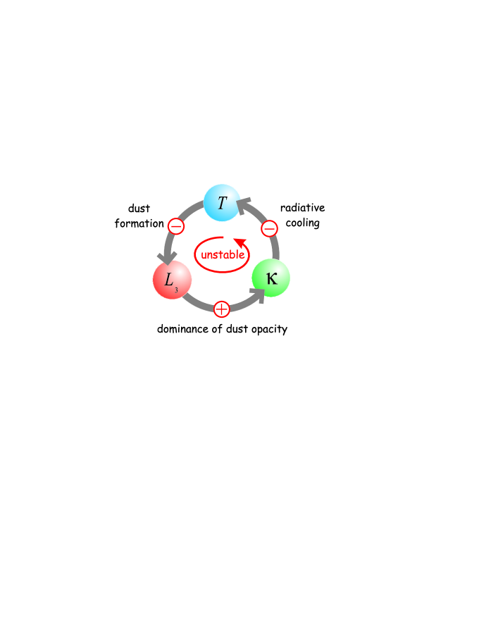
Figure 1: Unstable feedback loop in dust forming systems: Dust, once formed, increases the total opacity which intensifies radiative cooling. The temperature decreases and enters the dust formation window. Therefore, more dust is formed which increases the opacity further. An instability establishes where the dust improves the conditions for its own formation hel2003.

Carrying out numerical simulations of the whole time-dependent system of model equations (Eqs. 1 – 3, 8, 9), turbulence is seen as acoustic waves being by-products of colliding convective cells holks2001b which undergo an adiabatic increase of size during their upward travel through the substellar atmosphere. A feedback loop establishes in a dust-forming system in which interacting expansion waves play a key role (Fig. 1): The interaction of small-scale disturbances of the fluid field can cause a local and temporarily limited temperature decrease low enough to initiate dust nucleation. These seed particles grow until they reach a size where the dust opacity is large enough to accelerate radiative cooling which causes the temperature to decrease again below a nucleation threshold ($T_{\rm s}$). Dust nucleation is henceforth re-initiated which results in a further intensified radiative cooling. The nucleation rate and consequently also the amount of dust particles increase further. This run-away process is stopped if either the radiative equilibrium temperature of the gas is reached or all condensible material is consumed. Meanwhile, the seed particles have grown to macroscopic sizes.

The result is a highly variable dust distribution in space and time on the microscopic scales investigated (e. g. $\Delta l\approx 10^{2}$ cm, $\Delta t\approx 0.5$ s) due to the occurrence of singular nucleation events. It is immediately clear, that such scales are not easily resolvable by observations, but these are the scales on which structure formation is likely to be initiated. However, such small scale pattern might move and successively initiate dust formation at various sites in the atmosphere. A larger and larger cloud structure may thereby form which is, hence, determined by a non-local hydrodynamic coupling whereas at each site the above outlined local feedback loop will act (compare Fig. 3).

3.3 Mesoscopic regime

Following Kolmogoroff’s idea, the mesoscopic scales shall be considered as those where energy is only transfered through the turbulence cascade, but is not injected or dissipated. Convective elements are generated as long as the Schwarzschild criteria is fulfilled in the substellar atmosphere. The inertia of mass will drive the convective elements beyond Schwarzschild’s boundary, a phenomenon usually named as overshooting, which extends this zone further. The mass elements interact, collide, and transfer part of their energy into small scale structures, thereby producing a whole spectrum of them being viewed as waves or – turbulence elements. These waves propagate and enter even atmospheric regions which are not influenced by convective motions any more.

The question arises how the dust formation process takes place in such a stochastically fluctuating thermo- and hydrodynamic environment, and therefore which influence such small scale disturbances may have on the whole atmospheric structure and the formation of large scale pattern possibly responsible for observed variabilities. A model for driven turbulence was proposed hkws2002; hkwns2003 which simulates a constantly occurring, small-scale energy input assumed to originate from a convectively active zone. Following Reynolds scale separation ansatz a background field $\alpha_{0}({\boldsymbol{x}},t)$ is disturbed by a fluctuation $\delta\alpha({\boldsymbol{x}},t)$ of some variable $\alpha({\boldsymbol{x}},t)$ such that

$$\alpha({\boldsymbol{x}},t)=\alpha_{0}({\boldsymbol{x}},t)+\delta\alpha({\boldsymbol{x}},t).$$ (10)

$\alpha(\boldsymbol{x},t)\,\epsilon\,\{\boldsymbol{u}(\boldsymbol{x},t),P(\boldsymbol{x},t),S(\boldsymbol{x},t)\}$ ($\boldsymbol{u}(\boldsymbol{x},t)$ - velocity, $P$ - pressure, $S$ - entropy). The velocity fluctuation $\delta\boldsymbol{u}({\boldsymbol{x}},t)$ follows the Kolmogoroff spectrum in $k$-space in which a whole range of wavenumbers is excited ($k_{\rm min}=2\pi/l_{\rm max}$, $k_{\rm max}=2\pi/(3\Delta x)$, $l_{\rm max}=5\times 10^{4}$cm – maximum scale considered, $\Delta x=10^{2}$cm – spatial grid resolution). The model for driven turbulence relies on a superposition ansatz of different wave modes and therefore allows again to carry out direct simulation of the time and space evolution of the dust complex, now in a stochastically excited medium typical for the elswise dust-hostile part of a brown dwarf atmosphere.

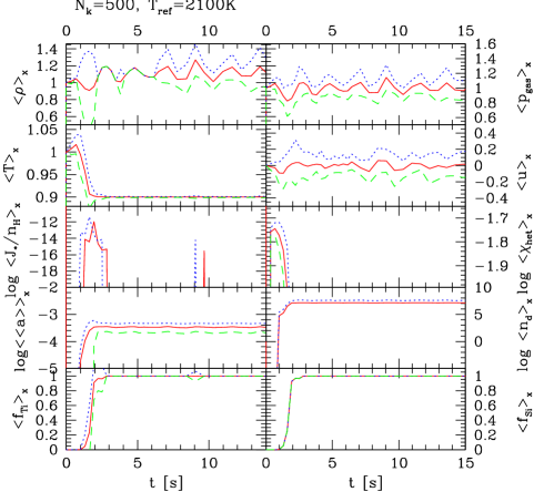
Figure 2: Fluctuating dust component in substellar atmospheres. The space-means $\langle\alpha(t)\rangle_{x}$ (solid/red) with the apparent standard deviations $\sigma_{\rm N_{x}-1}^{\alpha}(t)$ (dotted/dashed) as function of time for $T_{\rm ref}=2100$K, $\rho_{\rm ref}=3.16\,10^{-4}$g cm^-3, $v_{\rm ref}=c_{\rm S}/10$. ($\langle\alpha(t)\rangle_{x}+\sigma_{\rm N_{x}-1}^{\alpha}(t)$ - dotted/blue; $\langle\alpha(t)\rangle_{x}-\sigma_{\rm N_{x}-1}^{\alpha}(t)$ - dashed/green).

Nucleation events and nucleation fronts

An initially hydrodynamically homogeneous and dust-free, 500m-sized gas parcel has been considered in a deep layer of a brown dwarf atmosphere initially too hot for nucleation. The gas is disturbed by superimposed waves entering through its boundaries. If these disturbances carry already a temperature below the nucleation threshold ($T_{\rm s}$ - nucleation threshold temperature), a nucleation front will develop: The nucleation peak moves inwards together with the wave and initiates the feedback loop already known from the microscopic regime by leaving behind first dust seeds. If the entering temperature disturbances is not enough to cross $T_{\rm s}$, interaction with some expansion wave coming from another direction at some time and some site will take place thereby causing singular nucleation events to occur.

A nucleation front tends to homogeneously fill the gas parcel with dust in 1D situations while nucleation events cause a more heterogeneous dust distribution due to their short life time. In more than 1D, also nucleation fronts cause a heterogeneous dust distribution because their ’parent’ waves will interact and influence the conditions for dust formation.

Large variations in the dust quantities occur when the formation process starts to influence the hydro- and thermodynamics of the gas parcel. If all available material has been consumed, the mean dust quantities reach an almost constant values (Fig. 2) at a certain place in the atmosphere which is characterized by $T_{\rm ref}$. During this active time ($\Delta t\approx 3\,$s), the variation in the number of dust particles is $\cal{O}$$(10^{5}\,$cm${}^{-3})$ and in the mean particle size $\cal{O}$$(10^{2}\,\mu$m). The variation of the density is considerable (see standard deviations in Fig. 2) during the time of temperature decrease which assures the establishment of the pressure equilibrium.

A convectively ascending, initially dust free gas element can be excited to form dust by waves running through it. A cloud can therefore be fully condensed at much higher temperatures than classically expected, i. e. in an undisturbed case.

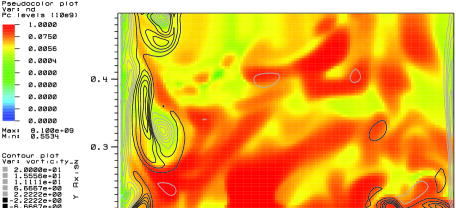
Figure 3: Spatial appearance of the number of dust particles ($\log n_{\rm d}$ [cm^-3]; false color background) and the vorticity ($\nabla\times\boldsymbol{v}$; black and grey contour lines) of the 2D velocity field for $t=0.8$s of a simulation with $T_{\rm ref}=2100$ K, $\rho_{\rm ref}=3.16\,10^{-4}$g cm^-3, $v_{\rm ref}=c_{\rm S}$.

Formation of large scale structures in 2D

2D simulations with the smallest eddy size being $\lambda^{\rm 2D}_{\rm min}=5\,$m, the largest are of the size of the gas box $\lambda^{\rm 2D}_{\rm max}=500\,$m, reveal a very intermittent distribution of the dust in space during the time of efficient dust formation (Fig. 3). The very inhomogeneous appearance of the dust complex is a result of nucleation fronts and nucleation events comparable to the 1D results. The nucleation is now triggered by the interaction of eddies coming from different directions. Large amounts of dust are formed and appear to be present in lane-like structures (large $\log\,$n_d; dark/red areas in Fig. 3). The lanes are shaped by the constantly inward traveling waves. Our simulations show that some of the small scale structure merge thereby supporting the formation of lanes and later on even larger structures.

Dust is also present in curled structure which indicates the formation of vortices due to the 2D waves driving turbulence. As the time proceeds in the 2D simulation, vortices develop orthogonal to the velocity field which show a higher vorticity ($\nabla\times\boldsymbol{u}(\boldsymbol{x},t)$) than the majority of the background fluid field. Comparing the distribution of dust particles (false color background in Fig. 3) with the vorticity (contour lines in Fig. 3), shows that the vortices with high vorticity preferentially occur in dust free regions or regions with only little amounts of dust present. These vortices can efficiently drag the dust into regions with still material available for further condensation shaping thereby larger and larger structures.

4 Dust formation on large scales

The atmospheric extension ($\approx 100\,$km – several pressure scale heights $H_{p}$) proposes a natural upper limit for the macroscopic scale regime. On this scale, the interplay between convective overshooting and gravitational settling (drift) is a major mechanism which influence the dust structure of the whole atmosphere. Since the dust is strongly coupled to the hydro- and thermodynamics of the atmosphere, gravitational settling and convective overshooting indirectly alter the atmospheric density and temperature structure which are important for the spectral appearance of the objects. The large scale structures are those which are usually accessible by observations. Therefore, the understanding and modeling of processes directly connected with macroscopic scale motions are of particular interest.

4.1 The model of a quasi-static dust layer

A theoretical consistent description of dust formation, gravitational settling, and element depletion (Eqs. 7, 9) was needed in order to understand the formation and the structure of dust cloud layers which is urgently needed for explaining the spectral appearance of Brown Dwarfs wh2003a. A first application to the quasi-static case of a brown dwarf atmosphere calculation was carried out by providing a model of a quasi-static cloud layer, i.e. ${\boldsymbol{v}}_{\rm gas}=0$ and $\frac{\partial L_{j}}{\partial t}=0$ in Eqs. (1) – (3), (7), (9) wh2003b. However, if ${\boldsymbol{v}}_{\rm gas}=0$ Eqs. (7) have the trivial solution $L_{j}\!\equiv\!0$ (see Sect. 2). The physical interpretation of this solution is that dust grains have once formed in the sufficiently cool layers, have consumed all available condensible elements up to the saturation level, and have finally left the model volume by gravitational settling. Consequently, a truly static atmosphere must be dust-free which – in this generality – contradicts the observations.

This picture changes, however, if we take into account a mixing of the atmosphere caused by the convection. This mixing leads to an ongoing replenishment of the gas with fresh, uncondensed matter from the deep interior of the brown dwarf, which can counterbalance the loss of condensible elements via the formation and gravitational settling of dust grains. Thus, a convective mixing can maintain a stationary situation:  Seed particles nucleate in metal-rich, i. e. supersaturated upwinds. Dust particles grow on top of these nuclei by the accretion of molecules and rain out as soon as they have reached a certain size. The sinking grains will finally reach deeper atmospheric layers which are hot enough to cause their thermal evaporation, which completes the life cycle of a dust grain in a brown dwarf atmosphere. We therefore enlarge the static case of our model by a simple description of the convective mixing such that the stationary dust moment equations write

$$-\frac{d}{dz}\!\!\left(\frac{L_{j+1}}{c_{T}}\right)\;=\;\frac{1}{\xi_{\rm lKn}}\left(-\frac{\rho L_{j}}{\tau_{\rm mix}}+{V_{\ell}}^{\,j/3}J_{\star}+\frac{j}{3}\chi_{\rm lKn}^{\rm net}\,\rho L_{j-1}\right)$$ (11)

with algebraic auxiliary conditions

$$\frac{n_{\langle{\rm H}\rangle}(\epsilon_{i}^{0}-\epsilon_{i})}{\tau_{\rm mix}}\;=\;\nu_{i,0}\,{N_{\ell}}\,J_{\star}\,+\,\sqrt[3]{36\pi}\,\rho L_{2}\sum\limits_{r=1}^{R}\nu_{i,r}n_{r}v^{\rm rel}_{r}\alpha_{r}\left(1-\frac{1}{S_{r}}\right)\ .$$ (12)

According to this approach, the gas/dust mixture in the atmosphere is continuously replaced by dust-free gas of solar abundances on a depth-dependent mixing time-scale $\tau_{\rm mix}(z)$, which can be adapted to a convection model (see discussion in wh2003b; wh2003c). $\epsilon_{i}$ is the actual abundance of element $i$ in the gas phase and $\epsilon_{i}^{0}$ its solar value ag89. By fitting the mass exchange frequency of 3D dynamic simulations of surface convection by lah2002 with an exponential we can apply a rough description of $\tau_{\rm mix}(z)$.

4.2 Numerical approach

Equation (11) is a system of ordinary differential equations of first order which can be solved by standard numerical methods. The differential equations are integrated inward by means of the variable transformation $z^{\prime}\!=\!z_{\rm max}-z$ using the Radau 5 – solver for stiff ordinary differential equations hw91a). For test purposes, the equation of hydrostatic equilibrium $dP_{\rm gas}/dz=-\rho g$ is solved in addition to the three moment equations (11), where the actual gas pressure $P\!=\!\sum_{i}n_{i}kT$ results from the chemical equilibrium calculations. The integration is stopped as soon as one of the dust moments becomes negative, indicating that the dust has completely evaporated.

4.3 Structure of a quasi-static cloud layer

The vertical structure of the cloud layer results from a competition between the four relevant physical processes: mixing, nucleation, growth/evaporation and drift. Following the cloud structures inward (from the left to the right in Fig. 4) roughly five different regions can be distinguished, marked by the Roman digits, which are characterized by different leading processes concerning the dust component.

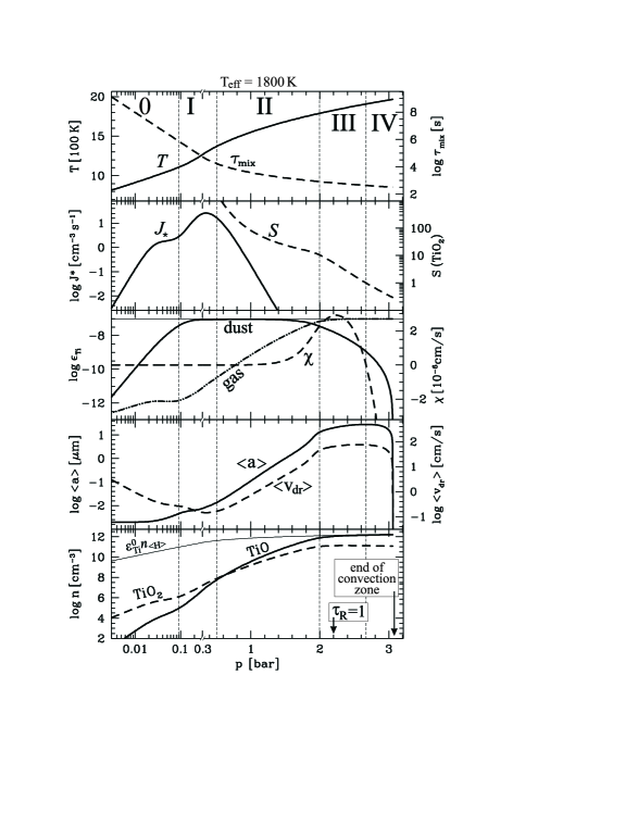
Figure 4: Calculated TiO₂ cloud structures for models with $\log\,g=5$ and $T_{\rm eff}=1800\,$K. Note the scaling of the partly logarithmic and partly linear $p$-axis. 1^st panel: prescribed gas temperature $T$ (solid), according to Tsuji (2002), and mixing time-scale $\tau_{\rm mix}$ (dashed). 2^nd panel: nucleation rate $J_{\star}$ (solid) and supersaturation ratio $S_{\rm TiO_{2}}$ (dashed). 3^rd panel: Ti abundance in the dust phase $\epsilon^{\rm dust}_{\rm Ti}$ (solid) and in the gas phase $\epsilon_{\rm Ti}$ (dashed-dotted). The solar value $\epsilon_{\rm Ti}^{0}$ is additionally indicated by a thin straight line. The dashed line shows the growth velocity $\chi^{\rm net}_{\rm lKn}$. 4^th panel: mean particle size $\langle a\rangle\!=\!\sqrt[3]{3/(4\pi)}\,L_{1}/L_{0}$ (solid) and mean drift velocity $\langle v_{\rm dr}\rangle\!=\!\sqrt{\pi}g\rho_{\rm d}\langle a\rangle\,/\,(2\rho c_{T})$ (dashed, see Eq. (66) in Paper II). 5^th panel: molecular particle densities of TiO (solid) and TiO₂ (dashed). For comparison, the hypothetical total titanium nuclei density for solar abundances $n_{\langle{\rm H}\rangle}\epsilon^{0}_{\rm Ti}$ is depicted by a thin solid line.

0. Dust-poor depleted gas: High above the convection zone, the mixing time-scale is large and the elemental replenishment of the gas is too slow to allow for considerable amounts of dust to be present in the atmosphere. The few particles forming here are very small $\langle a\rangle\!<\!10^{-2.5}\,\mu$m and have drift velocities $\langle v_{\rm dr}\rangle\approx 1\,$mm/s to 1 cm/s which causes these atmospheric layers to become dust-poor. The gas phase is strongly depleted in condensible elements. The Ti abundance in the gas phase $\epsilon_{\rm Ti}$ is reduced by a factor between $10^{5}$ and $10^{7}$ from its solar value. However, phase equilibrium ($S\!=\!1$) is not achieved because even the very small disturbance of the atmosphere by mixing is sufficient to produce a solution which differs significantly from the trivial solution in the truly static case.

I. Region of efficient nucleation: Nucleation takes place mainly in the upper parts of the cloud layer, where the temperatures are sufficiently low and the elemental replenishment by mixing is sufficiently effective. Although the gas is strongly depleted in heavy elements in these layers, it is nevertheless highly supersaturated ($S\!>\!1000$) such that homogeneous nucleation can take place efficiently. Since very many seed particles are produced in this way, the dust grains remain small $\langle a\rangle\!<\!0.01\,\mu$m and have small mean drift velocities $\langle v_{\rm dr}\rangle\approx 0.1\,$mm/s … $1\,$mm/s, which are even smaller than in region 0 because of the higher gas densities.

II. Dust growth region: With the inward increasing temperature, the supersaturation ratio $S$ decreases exponentially which leads to a drastic decrease of the nucleation rate $J_{\star}$. Consequently, nucleation becomes unimportant at some point, i. e. the in-situ formation of dust particles becomes inefficient in region II. Here, the condensible elements mixed up by convective overshoot are mainly consumed by the growth of already existing particles, which have formed in region I and have drifted into region II. The gas is still strongly supersaturated $S\!\gg\!1$, indicating that the growth process remains incomplete, i. e. the condensible elements provided by the mixing are not exhaustively consumed by growth. The dust component in region II is characterized by an almost constant degree of condensation ($\propto\!\epsilon^{\rm dust}_{\rm Ti}\!\propto\!L_{3}\!\approx\!{\rm const}$), while the mean particle size $\langle a\rangle$ and the mean drift velocity $\langle v_{\rm dr}\rangle$ increase inward. Consequently, the total number of dust particles per mass ($L_{0}$) and their total surface per mass ($\propto\!L_{2}$) decrease.

III. Drift dominated region: With the decreasing total surface of the dust particles ($\propto\!L_{2}$), the consumption of condensible elements from the gas phase via dust growth becomes less effective. At the same time, due to the increase of the mean particle size $\langle a\rangle$, the drift velocities increase. When the dust particles have reached a certain critical size, $\langle a\rangle_{\rm cr}\!\approx\!15\,\mu$m to $50\,\mu$m, the drift becomes more important than the growth, and the qualitative behavior of the dust component changes. This happens at the borderline between region II and III, which we denote by rain edge. Although the gas is still highly supersaturated $S\!\approx\!1\,...\,10$, the in-situ formation of dust grains is ineffective as in region II. The depletion of the gas phase vanishes in region III, i. e. the gas abundances approach close-to-solar values. The grains reach their maximum radii at the lower boundary of region III (the cloud base): $\langle a\rangle\approx\!30\,\mu$m to $400\,\mu$m at maximum drift velocities.

IV. Evaporating grains: The gravitationally settling dust particles finally cross the cloud base and sink into the undersaturated gas situated below, where $S\!<\!1$. Here, the dust grains raining in from above evaporate thermally. The evaporation of these dust particles, however, does not take place instantaneously, but produces a spatially extended evaporation region IV with a thickness of about 1 km. With decreasing altitude, the particles get smaller $d\langle a\rangle/dz\!<\!0$ and slower $d\langle v_{\rm dr}\rangle/dz\!<\!0$. Consequently, their residence times increase, and a run-away process sets in which finally produces a very steep decrease of the degree of condensation, terminated by the point where even the biggest particles have evaporated completely. We note that region IV, in particular, cannot be understood by stability arguments, but requires a kinetic treatment of the dust complex.

5 Conclusions

The dust formation in brown dwarfs atmospheres is a multi-scale problem where different physical mechanisms characterize the different scale regimes:

• In the microscopic scale regime, single acoustic waves interact, thereby initiate dust formation.

• The superposition of a whole spectrum of turbulence elements determine the mesoscopic scale regime resulting in a highly fluctuating fluid field.

• The interplay of gravitational settling of dust grains and the convective up-mixing of uncondensed material governs the macroscopic scale regime.

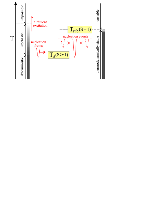
Figure 5: Regimes of turbulent dust formation. $T_{S}$: nucleation threshold temperature (supersaturation $S\ll 1$ required), $T_{\rm sub}$: sublimation temperature.

The main scenario envisioned is a convectively ascending fluid element in a brown dwarf atmosphere, which is excited by turbulent motions and just reaches sufficiently low temperatures for condensation. The dust formation in a turbulent gas is found to be strongly influenced by the existence of a nucleation threshold temperature $T_{S}$. The local temperature $T$ must at least temporarily decrease below this threshold in order to provide the necessary supersaturation for nucleation, e.g. by eddy interaction.

Depending on the relation between the local mean temperature $\overline{T}$ and $T_{S}$, three different regimes can be distinguished (see l.h.s. of Fig. 5): (i) the deterministic regime ($\overline{T}<T_{S}$) where dust forms anyway, (ii) the stochastic regime ($\overline{T}>T_{S}$) where $T<T_{S}$ can only be achieved locally and temporarily by turbulent temperature fluctuations, and (iii) a regime where dust formation is impossible. The size of the stochastic regime depends on the available turbulent energy. This picture of turbulent dust formation is quite different from the usually applied thermodynamical picture (r.h.s. in Fig. 5) where dust is simply assumed to be present whenever $T<T_{\rm sub}$, where $T_{\rm sub}$ is the sublimation temperature of a considered dust material.

After initiation, the dust condensation process is completed by a phase of active particle growth until the condensible elements are consumed, thereby preserving the dust particle number density for long times. However, radiative cooling (as follow-up effect) is found to have an important influence on the subsequent dust formation, if the dust opacity reaches a certain critical value. This cooling leads to a decrease of $\overline{T}(t)$ which may re-initiate the nucleation. This results in a runaway process (unstable feedback loop) until radiative and phase equilibrium is achieved. Depending on the difference between the initial mean temperature $\overline{T}(t\!=\!0)$ and the radiative equilibrium temperature $T_{\rm RE}$, a considerable local temperature decrease and density increase occurs. Since the turbulent initiation of the dust formation process is time-dependent and spatially inhomogeneous, considerable spatial variations of all physical quantities (hydro-, thermodynamics, dust) occur during the short time interval of active dust formation (typically a few seconds after initiation), which actually creates new turbulence. Thus, small turbulent perturbations have large effects in dust forming systems. Our 2D simulations show that the dust appears in lane-like and curled structures. Small scale dust structures merge and form larger structures. Vortices appear to be present preferentially in regions without or with only little dust. Non of these structures would occur without turbulent excitation.

From our work on small-scale turbulence simulations of dust-hostile regions in substellar atmospheres, we compile necessary criteria for a subgrid model of a dust forming, turbulent system.

Criteria on a subgrid model of a turbulent, dust-forming system: a) The subgrid model should describe the transition stochastic $\rightarrow$ deterministic regime in dust forming turbulent fluids. b) The dust formation process (nucleation + growth) is restricted to a short time interval since the dust formation time scales are much smaller than the large-scale hydrodynamic time scales.
This involves that: $\bullet$ The nucleation does occur only locally and event-like in very narrow time slots. $\bullet$ The growth process continues as long as condensible material is available. $\bullet$ The condensation process freezes in and the inhomogeneous dust properties are preserved. $\bullet$ Almost constant characteristic dust properties result in the mean-long term behavior. c) The feedback loop with its fast radiative cooling should govern the transition from an almost adiabatic to an isothermal behavior of the dust/gas mixture.

The largest, observable scale of a brown dwarf atmosphere has been investigated by attacking the drift problem. A consistent theoretical description was derived for dust formation and destruction, gravitational settling, and element depletion including the effect of convective overshoot. It was therewith possible for the first time to overcome the widely used concept of ad hoc dust presents in substellar atmospheres. Test calculations have shown that the dust will appear stratified in the atmosphere causing a corresponding depletion of the gas phase.

Acknowledgements: This work has been supported by the DFG (grants SE 420/19-1,2; Kl 611/7-1; Kl 611/9-1) as part of the DFG-Schwerpunkt Analyse und Numerik von Erhaltungsgleichungen.