Evidence for Low-Dimensional Chaos in Semiregular Variable Stars

Abstract

An analysis of the photometric observations of the light curves of the five large amplitude, irregularly pulsating stars R UMi, RS Cyg, V CVn, UX Dra and SX Her is presented. First, multi-periodicity is eliminated for these pulsations, i.e., they are not caused by the excitation of a small number of pulsation modes with constant amplitudes. Next, on the basis of energetics we also eliminate stochasticity as a cause, leaving low dimensional chaos as the only alternative. We then use a global flow reconstruction technique in an attempt to extract quantitative information from the light curves, and to uncover common physical features in this class of irregular variable stars that straddle the RV Tau to the Mira variables. Evidence is presented that the pulsational behavior of R UMi, RS Cyg, V CVn and UX Dra takes place in a 4-dimensional dynamical phase space, suggesting that two vibrational modes are involved in the pulsation. A linear stability analysis of the fixed points of the maps further indicates the existence of a two-mode resonance, similar to the one we had uncovered earlier in R Sct:  The irregular pulsations are the result of a continual energy exchange between two strongly nonadiabatic modes, a lower frequency pulsation mode and an overtone that are in a close 2:1 resonance. The evidence is particularly convincing for R UMi, RS Cyg and V CVn, but much weaker for UX Dra. In contrast, the pulsations of SX Her appear to be more complex and may require a 6D space.

¹Physics Department, University of Florida, Gainesville, FL, USA; buchler@phys.ufl.edu
²Konkoly Observatory, Budapest, HUNGARY; kollath@konkoly.hu
²Department of Physics, Grinnell College, Grinnell, IA 50112, USA

1. INTRODUCTION

The five stars considered here are pulsating variables and show the sorts of light curve irregularities that are generally associated with classification as semiregular variables. The measurements section of the SIMBAD database lists V CVn, R UMi, and RS Cyg as SRa stars, UX Dra as SRb, and SX Her as SRd, although conflicting classifications exist. RS Cyg and UX Dra are also classified as carbon stars. SX Her is earlier in spectral type (K2) than the others (late M or C).

V CVn has been reported to have two closely spaced periods (Loeser et al. 1986, Kiss et al. 1999, Kiss et al. 2000) and exhibits time-dependent polarization (Boyle et al. 1986, Magalh es et al. 1986). SX Her is a metal-poor star (Preston and Wallerstein 1963) that shows no signs of an infrared excess (Carney et al. 2003). Its period is apparently changing slowly (Percy and Kolin 2000).

In §3 we argue on physical grounds that the irregular pulsations of these stars cannot be multi-periodic as has been suggested (Kiss et al. 1999), nor can they be of a stochastic nature as proposed in Konig et al. (1999). This means that, by default, they therefore must be chaotic. If the light curve is indeed unsteady because of a chatic dynamics, then it is not astonishing that an interpretation within a traditional periodic framework would lead to a spurious conclusion that there are closely spaced peaks or that the period is changing (Buchler, J. R. & Kolláth, Z., 2001).

In §4 we apply a global flow reconstruction (e.g., Serre et al. 1996) to the data. This tool has been specifically designed for the study of chaotic signals which have only a few degrees of freedom (low dimensional chaos). We show that this reconstruction can capture the pulsation dynamics of these stars. The fact that the reconstruction allows us to generate synthetic LCs with properties similar to the observed LCs thus provides additional, a posteriori evidence for low dimensional chaos.

The global flow reconstruction also yields quantitative information about the underlying dynamics, such as its dimension. We can use this information to uncover the physical nature of the irregular LCs of these stars. In particular, it allows us to address the question of whether the same resonant mechanism is operative here as in the case of the RV Tau-type star R Scuti where the large amplitude irregular pulsations were shown to be a consequence of the resonant excitation of an overtone with close to double the frequency of the basic pulsation mode under highly nonadiabatic conditions (Buchler et al. 1995, 1996). The fundamental mode is self-excited and wants to grow, whereas the entrained, resonant overtone is stable and wants to decay, from which a chaotic motion of alternating growth and decay ensues, a scenario known in nonlinear dynamics under the name of Shilnikov (e.g., Bergé et al. 1986).

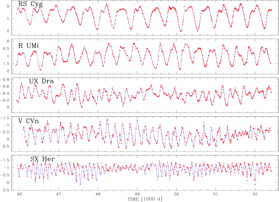
Figure 1.— Light curves (mag). Dots: Observed LCs (Cadmus); solid lines: fits to LCs, binned and averaged over 10 d, and smoothed with $\sigma_{s}=0.01$ (see text); Time = Julian date 2400000 + [1000 days].

2. Observations

Our analysis is based on high quality V band light curve (LC) data from the observational program at Grinnell College that span close to 18 years. The observations were made with the 0.61 m telescope at the Grant O. Gale Observatory using a conventional photoelectric photometer. The data were reduced differentially relative to the following comparison stars (in parentheses after the associated variable star): R UMi (HD 150747), RS Cyg (HD 192422), V CVn (HD 116531), UX Dra (HD 178089), SX Her (HD 145226). The comparison stars were monitored relative to additional check stars and found to exhibit no significant variability. The reduction included corrections for atmospheric extinction and transformation to the UBV system using B band data that are not presented here. The precision of the data is determined primarily by atmospheric conditions but can be estimated to be about 0.01 magnitude from the repeated measurements that make up a single data point as well as from related data.

Because continuity of the data is important for the sort of analysis presented here, efforts were made to essentially eliminate the gaps between observing seasons by taking some data (a small fraction of the total) at larger airmasses and in brighter twilight than is desirable for photometric observations. The quality of the data obtained in twilight was improved by modeling the nonlinear time variation in the sky brightness. Although the quality of the measurements obtained under these conditions is a bit worse than that for data taken under more favorable conditions, it is still good enough for the purposes of this paper and is far preferable to gaps in the data. The data are available from RRC.

The observed LC data are displayed as dots, jointly with the smoothed fits, in Fig. 1. The sampling is irregular with an average spacing of   10 d. The light curves of R UMi, V CVn, and UX Dra exhibit sizeable vertical shifts that could be due to dust formation during the pulsation but, as the next section suggests, they could also be part of the intrinsic pulsation dynamics of the stars. The LC of SX Her shows large fluctuations in overall amplitude. RS Cyg displays distinctive dips at the maxima of its LC.

3. THE NATURE OF THE PULSATIONS

3.1. Time-Frequency Analysis

Figure 2, we present a comparison of the photoelectric Cadmus data and the combined visual amateur astronomer data (AAVSO, AFOEV, BAAVS, VSJSO) of V CVn for approximately the same time-intervals. These smoothed time-series therefore have a different zero points and different amplitudes, and they also have quite a different quality. (The smoothings that we apply to these data will be discussed below.)

We display the smoothed LCs (top), the amplitude Fourier spectra (FS) (right) and the time-frequency (TF) plots (Kolláth & Buchler 1996), also known as spectrograms. For the latter we have used the Zhao-Atlas-Marks (1990) kernel that belongs to a class of TFs known under the name of Reduced Interference Distributions (RIDs). These are designed to give much sharper images than the older transforms, such as Gábor, for example (e.g. Cohen 1994). In the TF plots we have enhanced the power at the harmonics to the same level as the fundamental to make it visible ($A(f)=A_{TF}(f)S(f)$, where $S=1$ for $f<1.1f_{0}$, where $f_{0}$ is the frequency of the fundamental peak, $S=5$, for example, for $f>1.9f_{0}$, and a linear increase in between). A comparison of the TF plots with the FS (on the right) clearly shows the size of this enhancement $S$.

Despite the fact that the Cadmus and amateur LCs are appreciably different at times, the TF plots are remarkably similar, showing their insensitivity to observational errors and to the smoothing procedure.

In Figs. 2 through 4 we display the TFs of RS Cyg, R UMi, UX Dra and SX Her. The TFs of all five stars show some amplitude (power) at twice the fundamental peak, and both RS Cyg and V CVn also have appreciable amplitude at $3f_{0}$. From the very appearance of the observed LCs one finds it hardly astonishing that for all five stars the instantaneous amplitudes in the dominant peaks waver in time, but more interestingly the instantaneous frequencies change as well. In addition, the first harmonic frequency peak does not change synchronously with that of the fundamental frequency. This asynchrony between the fundamental and the harmonic peaks rules out that all of the harmonic structure is due to the anharmonicity of the motion. Furthermore it cannot be explained by dust or spots, by binarity, by evolution or by stochasticity, even though all of these effects may be present and affect the LCs.

We shall first argue that the pulsations of these stars are neither periodic nor multi-periodic (see also Buchler & Kolláth 2003). Then we will give physical, energetic arguments that also eliminate a stochastic nature for these pulsations. This then, by default, leaves a low dimensional chaotic nature as the only alternative.

Figure 2.— V CVn: Left Figure: Cadmus photoelectric LC; Right Figure: combined visual amateur astronomer data. In each figure: Top: smoothed LCs, right: amplitude Fourier spectrum, center: time-frequency plot.

Figure 3.— Left Figure: RS Cyg: and Right Figure: R UMi. Top: smoothed LCs, right: amplitude Fourier spectra, center: time-frequency plots.

Figure 4.— Left Figure: UX Dra and Right Figure: SX Her. Top: smoothed LCs, right: amplitude Fourier spectra, center: time-frequency plota.

3.2. Multi-periodicity?

Because the ’multi-periodic’ label is sometimes used with different connotations, to be specific, we mean that the signal is such that (a) the FS contains a few discrete, basic frequencies, and all the other peaks correspond to linear combinations of these basic frequencies that arise because of nonlinear couplings, and (b) the amplitudes and frequencies of all these peaks are constant, or, at most, vary very slowly in time. The beat Cepheids and RR Lyrae are examples of this type of systems.

Multi-periodicity would thus imply that the major frequency peaks $f_{k}$ in the Fourier spectra are real and should correspond to actual pulsation frequencies or linear combinations thereof. Using these frequency peaks one can then make a multi-periodic fit $s(t)=\sum A_{k}sin(2\pi f_{k}t+\phi_{k})$ to the observational data. For the stars that we are considering we find that we need from 50 to 100 frequencies for a decent fit. This however poses a physical problem, namely the origin of these frequencies. Indeed, stellar modelling shows that there simply do not exist enough radial modes in the frequency range of interest for these types of star. This remains true even if allowance is made for nonradial modes with $\ell$ low enough (say $\ell=3$) to be observable photometrically and assuming that the latter can indeed be excited to such large amplitudes. Furthermore, typically only a few modes are found to be linearly unstable, and one would have to explain why so many other stable modes get entrained to such high amplitudes. We thus conclude that these LCs are not generated by a large set of excited pulsation modes.

There is still the possibility of a multi-periodic, but slowly evolving star. The structure of the peaks should thus changes slowly as well, but for our five stars the timespan of the observational data is too short compared to the evolutionary timescale. We note however, that for the RV Tau type star R Sct (Kolláth 1990), the frequencies in the FS appear randomly variable from one section of the data to another which thus also eliminates an explanation in terms of slowly evolving multi-periodic stars.

3.3. Stochasticity

A recent paper (Konig et al. 1999) claim to explain the irregular behavior of R Sct as the superposition of two stochastically excited damped linear oscillators. Typically stochastic excitation of vibrationally stable modes, such as the solar oscillations, leads to much smaller amplitudes. It seems more likely that pulsations as large as those observed in R Sct are due to a self-excited mode, such as in the Cepheid and RR Lyrae variables. In fact this brings us to our main rejection of stochastic excitation for R Sct. While such a stochastic ’explanation’ is perhaps correct from a mathematical point of view, it is not meaningful on physical grounds because no mechanism is proposed that could excite damped modes to such large pulsation amplitudes (up to factors of 40 in the LC of R Sct, for example).

In order to be more quantitative, let us consider a 0.7$M_{\odot}$ model with L=1000$L_{\odot}$ and $T_{\rm ef\!f}$=5300K (and X=0.726, Z=0.004). In our turbulent convective hydro-code (e.g., Kolláth et al. 2002) this model is unstable in the fundamental mode and leads to chaotic pulsations of alternating large and small amplitudes. The average pulsational kinetic energies in such typical cycles are $\langle$KE$\rangle$ = 0.31$\times 10^{42}$ and 0.23$\times 10^{42}$ ergs, respectively. The average turbulent energies are $\langle$TE$\rangle$ = 0.15$\times 10^{42}$ and 0.12$\times 10^{42}$ ergs, somewhat smaller, but of the same order within the accuracy of mixing-length models. The alleged stochastic excitation of Konig et al. (1999) can only be associated with the convective motions. Our numbers show that even if all available turbulent energy were converted into pulsational kinetic energy, there is barely enough energy. The pulsation is closely associated with a single (most likely radial) pulsation mode, or perhaps at most two of them, thus has a very directed form of kinetic energy. The amount of energy transferred ’stochastically’ from the kinetic energy associated with the largely disordered turbulent convection to these modes depends on the overlap integrals between the spatial distribution of the turbulent energy (e.g., Eqs. 6 and 7 of Buchler, Goupil & Kovács 1993). This overlap must be extremely small because of the very different nature of the two types of motion. Furthermore the power in the Fourier spectrum of turbulent convection at the pulsation frequency is very limited. This rules out stochasticity as the cause of the observed irregular behavior.

However, the amount of energy flowing through the pulsating envelope, viz. the product of the luminosity and the ’period’ $\sim$6.1$\times 10^{42}$ ergs, is almost 100 times the pulsation kinetic energy. This highly nonadiabatic situation certainly allows the observed changes in pulsational kinetic energy. A perhaps better estimate of the efficiency of conversion of heat into pulsation energy, or the percentage change of pulsation kinetic energy per cycle, is given by the linear growth-rates of the modes (e.g., $\kappa_{0}\times P_{0}\sim 1.25$ for the stellar model above). This is precisely what a chaotic dynamics is about: The nonlinear interaction of a small number of strongly nonadiabatic (dissipative) pulsation modes.

We conclude that it is therefore ultimately physics that rules out stochasticity for these stars. This is not to say, however, that superposed on the low dimensional radial chaotic dynamics, there cannot be stochastic motions, which furthermore are nonradial.

3.4. Other Reasons For Low Dimensional Chaos

There are additional reasons for believing that the pulsations of these five stars are chaotic and have a low dimension:  First, numerical hydrodynamic simulations, albeit of W Virginis type stellar models, uncovered the chaotic nature of the pulsations (Buchler & Kovács 1987, Aikawa 1987, Buchler, Goupil & Kovács 1987, Kovács & Buchler 1988, Letellier et al. 1996). Second, the analysis of the LC of the RV Tau-type star R Scuti clearly demonstrated the presence of a low dimensional chaotic pulsation dynamics (Buchler, Serre, Kolláth & Mattei 1995, Buchler, Kolláth, Serre & Mattei 1996). More recent work by other authors gives corroborating evidence for low dimensional chaos in large amplitude variabel stars (Kiss & Szatmáry 2002, Ambika et al. 2003).

Linear analyses are very useful for multi-periodic signals, but it is well known, at least outside astronomy, that for irregular, intrinsically nonlinear signals they yield limited information about the dynamics (e.g., Weigend & Gershenfeld 1994, Abarbanel et al. 1993). As we have already mentioned, a phenomenologically motivated multiperiodic fit will always be ’successful’ as an interpolation, but will give us not much information about the stellar pulsation aside from one or perhaps several average ’periods’. For the study such chaotic signals and for understanding the underlying dynamics a different approach is required.

A popular test for nonlinear behavior is the construction of first return maps (e.g., Ott 1993). For a dynamics with a fractal attractor with fractal dimension  $>$$\sim$ 2, such as the Rössler band, the first return maps show a tight parabolic structure, but for our stars they turn out to be essentially scatter diagrams. This negative result implies that, if this attractor is indeed fractal, the fractal dimension of the dynamics substantially exceeds a value of 2, and could even be greater than 3. We recall that for the star R Sct it was found that $d_{L}\sim 3.1$ (Buchler et al. 1996).

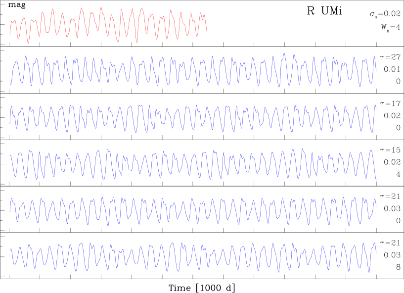
Figure 5.— R UMi, top: smoothed LC (mag); below: sections of synthetic LCs with various seeds and delays $\tau$ for maps constructed from the smoothed magnitude data; ($\tau$,$\sigma_{s}$,$W_{g}$) are indicated on the right ($W_{g}=0$ stands for no Gaussian filter);

Table 1 Linear stability properties of the fixed points of the maps ${\mathbf{\cal}M}$ for a selected subset of synthetic LCs with smoothings $\sigma_{s}$, $W_{g}$, delays $\tau$: Given are the the locations of the main fixed points $M_{fp}$, the growth rates $\kappa$, the frequencies $f$ and the ratios $f_{2}/f_{1}$. All frequencies and growth rates are in $[d^{-1}]$.

R UMi	$\sigma_{s}$	$W_{g}$	$\tau$	$M_{fp}$	$\kappa_{1}$	$f_{1}$	$\kappa_{2}$	$f_{2}$	$f_{2}/f_{1}$
	0.01	0	23	1.064	2.093E–03	3.543E–03	–3.275E–03	7.340E–03	2.07
	0.01	0	25	1.072	2.442E–03	3.504E–03	–3.635E–03	7.254E–03	2.07
	0.01	8	19	1.063	1.508E–03	3.532E–03	–2.712E–03	7.764E–03	2.20
	0.02	0	17	1.081	1.296E–03	3.511E–03	–2.112E–03	7.898E–03	2.25
	0.02	4	15	1.083	1.319E–03	3.523E–03	–2.146E–03	8.039E–03	2.28
	0.02	4	17	1.087	1.516E–03	3.539E–03	–2.188E–03	7.890E–03	2.23
	0.03	0	21	1.096	1.233E–03	3.554E–03	–2.696E–03	6.759E–03	1.90
	0.03	8	21	1.091	1.420E–03	3.547E–03	–3.231E–03	6.554E–03	1.85
RS Cyg:	$\sigma_{s}$	$W_{g}$	$\tau$	$M_{fp}$	$\kappa_{1}$	$f_{1}$	$\kappa_{2}$	$f_{2}$	$f_{2}/f_{1}$
	0.025	1	40	0.631	3.368E–03	2.793E–03	+1.981E–03	5.248E–03	1.88
	0.025	7	40	0.622	3.149E–03	2.793E–03	+1.830E–03	5.365E–03	1.92
	0.03	4	35	0.581	3.539E–03	2.701E–03	–5.122E–04	5.438E–03	2.01
	0.04	4	33	0.489	-1.142E-03	6.245E-03	2.398E-03	2.724E-03	2.29
	0.04	4	40	0.500	1.258E–03	2.708E–03	–9.522E–04	6.444E–03	2.38
	0.04	5	34	0.491	2.214E–03	2.724E–03	–1.062E–03	6.290E–03	2.31
V CVn:	$\sigma_{s}$	$W_{g}$	$\tau$	$M_{fp}$	$\kappa_{1}$	$f_{1}$	$\kappa_{2}$	$f_{2}$	$f_{2}/f_{1}$
	0.01	0	22	–0.279	–4.665E–03	5.102E–03	4.098E–03	1.119E–02	2.19
	0.01	6	22	–0.278	–4.514E–03	5.087E–03	4.005E–03	1.105E–02	2.17
	0.01	6	23	–0.263	–4.933E–03	5.065E–03	4.108E–03	1.047E–02	2.07
	0.01	12	21	–0.279	–4.665E–03	5.102E–03	4.098E–03	1.119E–02	2.19
	0.02	0	22	–0.279	–4.672E–03	5.076E–03	4.694E–03	1.108E–02	2.18
	0.02	6	21	–0.287	–4.448E–03	5.124E–03	4.309E–03	1.155E–02	2.25
	0.03	0	21	–0.292	–4.615E–03	5.115E–03	4.999E–03	1.152E–02	2.25
UX Dra:	$\sigma_{s}$	$W_{g}$	$\tau$	$M_{fp}$	$\kappa_{1}$	$f_{1}$	$\kappa_{2}$	$f_{2}$	$f_{2}/f_{1}$
	0.018	0	6	–0.39	–1.236E–02	3.963E–03	8.458E–03	5.975E–03	1.51
	0.016	0	5	–0.43	–9.825E–03	3.478E–03	5.684E–03	7.398E–03	2.13
	0.017	0	6	–0.41	–1.155E–02	3.720E–03	7.904E–03	6.423E–03	1.73
	0.018	0	6	–0.39	–1.236E–02	3.963E–03	8.458E–03	5.975E–03	1.51
	0.019	0	5	–0.39	–1.522E–02	3.633E–03	1.058E–02	5.548E–03	1.53

4. GLOBAL FLOW RECONSTRUCTION

Over the last decade we have developed a special tool for the analysis of irregular time-series, namely the global flow reconstruction technique (reconstruction technique for short). Our primary motivation has not been phenomenological, but rather has aimed for an understanding of the physical mechanism behind the irregular LCs of variable stars on the one hand, and for deriving qualitative and quantitative properties of this dynamics (Serre et al. 1996; reviewed in Buchler 1997, Buchler & Kolláth 2001; a similar approach was followed in other research areas, e.g., Gouesbet et al. 1997, Hegger et al. 1999).

Figure 6.— R UMi: LEFT: Amplitude FS top: of the smoothed LC, below: of synthetic LCs. RIGHT: corresponding Broomhead-King (BK) projections.

Only two very simple working assumptions underlie the reconstruction technique: (1) the LC is produced by the (deterministic) nonlinear interaction of a small number of pulsation modes, (2) the system is autonomous, i.e., explicit time-dependence, such as evolution over the span of the data, can be ignored.

A priori it may appear astonishing that one should be able to derive basic physical properties of the star from the mere knowledge of a scalar time-series, such as the LC. Yet, in the case of the star R Scuti it was possible to demonstrate that the irregular pulsations are the result of the nonlinear interaction between a self-excited pulsation mode that entrains a vibrationally stable mode through an approximate 2:1 resonance (Buchler et al. 1995, 1996).

The technique introduces a (Euclidean) reconstruction space of dimension $d_{R}$, in which one uses the observed time-series $s_{n}=s(t_{n})$ to construct successive position vectors

$${\bf~{}X_{n}}~{}=~{}(s_{n},~{}s_{n-\tau},~{}s_{n-2\tau},~{}\ldots,~{}s_{n-(d_{R}-1)\tau}).$$

The quantity $\tau$ is called the delay. Assumption (1) allows us to use the observed time-series to construct the best mathematical relationship ${\bf\cal M}$, (called a map or a flow in the case of a differential description), that evolves the system that produces the LC from one time-step to the next: $\quad{\bf X_{n+1}}={\bf\cal M}({\bf X_{n}}).\quad$ A dimension $d_{R}$ that is large enough to capture the dynamics of the pulsation is called an embedding dimension. Our goal is to find the minimum embedding dimension $d_{e}$. This dimension $d_{e}$ is not known a priori and it is one of the fundamental quantities that the analysis aims to determine. This dimension is important because it is closely related to the dimension $d$ of the actual ’physical’ phase space of the dynamics. For example, for a single oscillatory mode, $d$ would be equal to 2, for 2 coupled oscillatory modes $d=4$, and the involvement of a secular mode would add 1 to the dimension. Practice has shown that a multivariate polynomial functional form is suitable for the map ${\mathbf{\cal}M}$ and that polynomes up to order of 4 are generally sufficient; the coefficients of these polynomials are computed with a least-squares fit to the observed time-series (Serre et al. 1996). The reconstruction technique also introduces a delay $\tau$ which we consider a free parameter.

The reconstruction requires a time series with equal time intervals. Our data preparation is done in several steps:  (a) the data are binned and averaged over a time interval $\Delta t_{av}$. The typical time interval for the Cadmus data has a very broad peak around 10 d. In the following we have chosen values for $\Delta t_{av}$ = 10 d, except for UX Dra where we chose 1 d.  (b) The data are next smoothed with a cubic spline (Reinsch 1967) with a smoothing $\sigma_{s}$ which results in an equally spaced time series, with time intervals chosen to be 1 d. (c) Finally a moving Gaussian filter of width $W_{g}$ is applied to the splined time series.

Results of a preliminary analysis of these stars were reported in Buchler, Kolláth & Cadmus 2001. Here we perform a much broader analysis; in particular our search covers a wider range of smoothings, $\sigma_{s}$ and $W_{g}$. As a result we obtain firmer conclusions than were obtained in that paper.

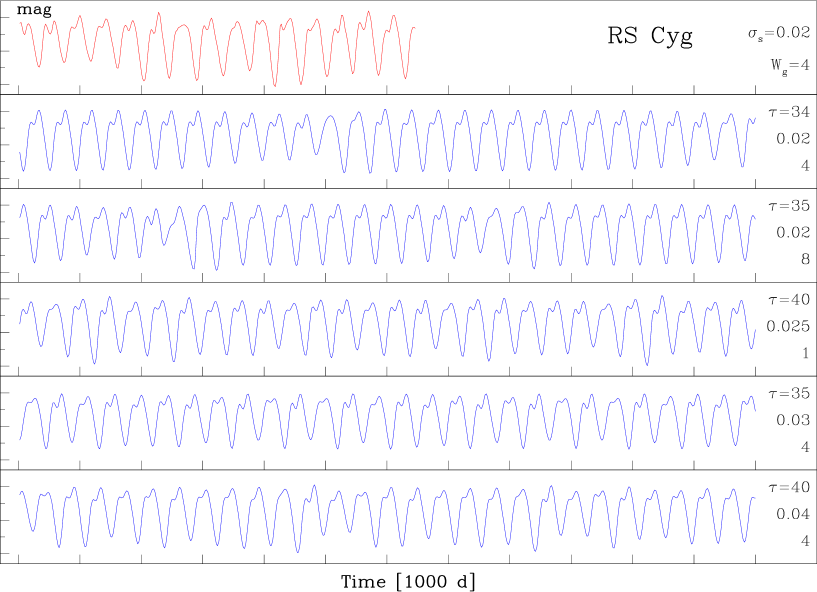
Figure 7.— RS Cyg, top: smoothed LC (mag); below: sections of synthetic LCs with various seeds and delays $\tau$ for maps constructed from the smoothed magnitude data; ($\tau$,$\sigma_{s}$,$W_{g}$) are indicated on the right;

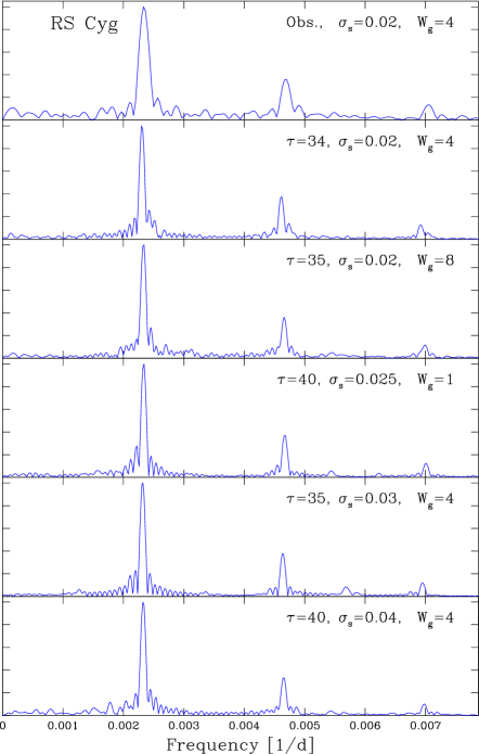
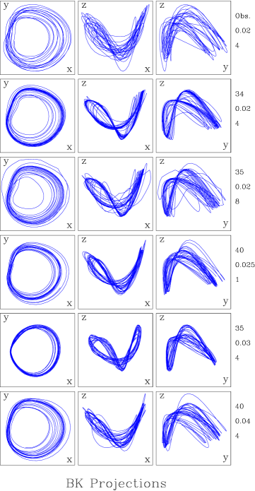
Figure 8.— RS Cyg: LEFT: Amplitude FS top: of the smoothed LC, below: of synthetic LCs. RIGHT: corresponding Broomhead-King (BK) projections.

4.1. R UMi

In this section we apply the reconstruction to the observed LC of R UMi, and concurrently we discuss some of the technical details of the reconstruction.

In Figure 5 on top we display a fit to the R UMi data, with the smoothing parameters $\sigma_{s}=0.02$ and $W_{g}=4$. Two observational points, at JD 46039.5095 and 46613.8169, give an unnatural looking wiggle in the smoothed data (e.g., in Fig. 1 of Buchler et al. 2001), and have therefore been omitted in the reconstructions. We have verified though that the reconstructions with all the observational points give essentially the same results, indicating a relative insensitivity of the R UMi reconstructions to individual points.

In practice, the reconstructions proceed as follows: from a smoothed light curve (with given $\sigma_{s}$ and $W_{g}$) a map ${\mathbf{\cal}M}$ is constructed for a given dimension $d_{R}$ and a given value of delay $\tau$. This map ${\mathbf{\cal}M}$ is then iterated from a seed value (chosen along the observed time-series) to generate what we call a synthetic LC. Actually, the map ${\mathbf{\cal}M}$ generates $d_{R}$ scalar sequences, namely the components of ${\bf X_{n}}$, shifted with respect to each other by $\tau$ days, but are essentially identical when superposed. This can be considered an a posteriori confirmation that the reconstruction is successful. For R UMi as for the other stars we have chosen 15000 d long iterations of which we typically discard the first three thousand days, because they may be transients in the evolution toward the chaotic attractor.

Because the data preparation obviously will have an effect on the reconstructed attractors, we therefore perform them for a range of smoothing and filtering values $\sigma_{s}$ and $W_{g}$. Ideally, we would also expect the results of the reconstructions to be independent of these smoothing parameters in some range of values (For a discussion of these issues we refer to Serre et al. 1996). In our surveys we perform the reconstructions with delays typically ranging from $\tau=4$ to 40 d. In a robust reconstruction the results should come out similar for some range of neighboring $\tau$ values.

It is obvious that for a successful reconstruction the data have to sample sufficiently well the dominant features of the dynamics in phase space. When the LC is very short – there are only 20 pulsation cycles for R UMi – the iteration of the constructed maps is not always stable and the synthetic LCs blow up. There can be several causes for such behavior, e.g., ’boundary crises’ (e.g., Ott 1993). In practice, we iterate a given map successively with different seeds until we obtain a synthetic LC of sufficient length and quality.

How do we judge the quality of the reconstruction?   There is no point in comparing chaotic signals point by point, but rather they need to be compared in a global or statistical sense. However, we are seriously hampered by the shortness of both the observed and synthetic LCs. We are therefore forced to rely on more subjective criteria.

Our first acceptance criterion relies on a visual comparison of the observed and synthetic LCs. When we attempt reconstructions for R UMi in 3D (i.e., with $d_{R}=3$), we find that the synthetic LCs bear no resemblance to the observed LC for any $\sigma_{s}$ or $W_{g}$. It is therefore immediately obvious that $d_{e}>3$.

In contrast, the 4D reconstructions show a relatively large insensitivity to the smoothing. We have made our survey with $\sigma_{s}=0.01$, 0.02, to 0.05 and $W_{g}=0$, 4 and 8 ($W_{g}$ =0 indicates that no Gaussian filter was applied). Good synthetic LCs have been obtained with between 3 and 9 delay values which, depending on the amount of smoothing, range from $\tau=15$ to 27 d. With larger smoothing, ($\sigma_{s}>0.03$), the reconstructions deteriorate, with the synthetic LCs becoming more symmetric about the average and more regular. Figure 5 displays a sample of our best segments of 4D synthetic LCs, with the delays $\tau$, and the smoothings $\sigma_{s}$ and $W_{g}$ indicated on the right. The fact that our 4D reconstructions appear to capture the dynamics of the pulsations of R UMi suggests that $d_{e}=4$.

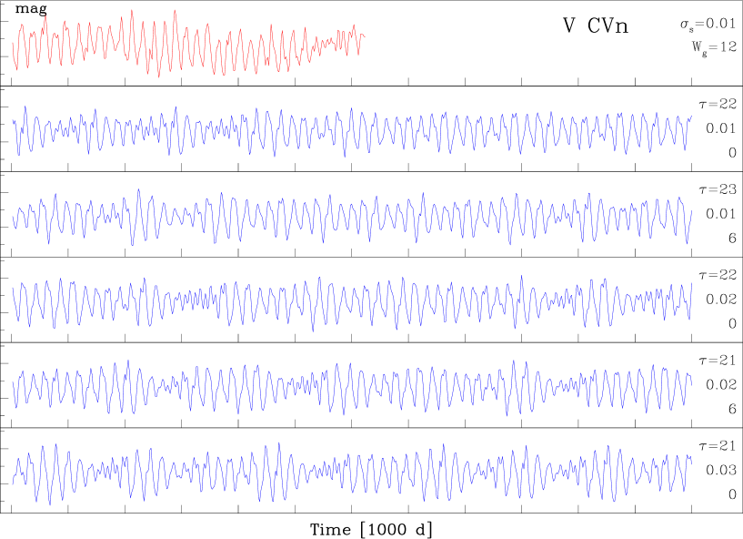
Figure 9.— V CVn: top: smoothed LC (mag); below: sections of synthetic LCs with various seeds and delays $\tau$ for maps constructed from the smoothed magnitude data; ($\tau$,$\sigma_{s}$,$W_{g}$) are indicated on the right $W_{g}=0$ stands for no Gaussian filter); below: sections of synthetic LCs with various seeds and delays $\tau$; maps constructed from the smoothed magnitude data;

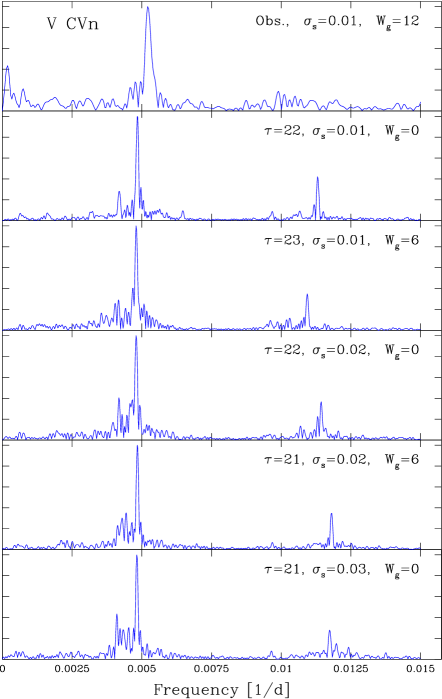
Figure 10.— V CVn: LEFT: Amplitude FS top: of the smoothed LC, below: of synthetic LCs. RIGHT: corresponding Broomhead-King (BK) projections.

A second comparison can be made at the level of the amplitude Fourier spectra (FS). Because the signals are unsteady, we do not want to compare individual peaks, but rather the FSs should have the same overall structure. Figure 6 displays successively from top to bottom, the FS of the smoothed and of our best synthetic LCs, indicating excellent agreement. The relative broadness of the fundamental peak for the observed LC is due to its shorter time span.

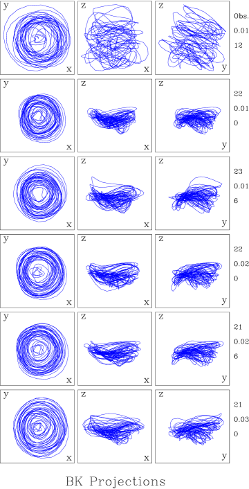
Figure 11.— V CVn: LEFT: Amplitude FS top: of the smoothed LC, below: of synthetic LCs. RIGHT: corresponding Broomhead-King (BK) projections.

Finally, a third comparison can be performed with BK projections (Broomhead & King 1987) which are the projections of the temporal signals on the first few eigenvectors of the auto-correlation matrix which represent an optimal visual way of spreading out the attractor. In practice, we first generate the projection matrix with the smoothed observed LC with a chosen delay $\tau$, and then use this matrix to make the projections of all the LCs. The BK projections onto the first three eigenvectors, labelled x, y and z, are displayed in Fig. 6, indicating that the structure of the reconstructed attractor is very similar to that of the observations.

The three tests indicate that, considering the extreme shortness of the data, the reconstructions for R UMi are quite good and reasonably robust.

In Table 1 we present the linear stability eigenvalues ($i2\pi f+\kappa$) of the fixed points of the maps. They should correspond to the frequencies of the modes that are excited in the pulsation and therefore to the stability of the equilibrium state of the star. Note that the value of the lowest frequency $f_{1}$ is close to the frequency of the lowest peak in the FS (0.00333$\pm$0.00003 d^-1). The frequency $f_{2}$ is not as well determined, although the frequency ratios are reasonably close to a 2:1 resonance.

Table 1 indicates that the growth rates are comparable to the frequencies, indicating the presence of extreme nonadiabaticy, consistent with the numerical modelling of such stars (Kovács & Buchler, 1988). Column 4 represents the values of the magnitude of the fixed point, i.e., the ’center of the motion’, which are close to the average magnitude of the observed LC, viz. 0.95, but not equal to it presumably because of the skewedness of the light curve. The growth rate $\kappa_{1}$ of the lower frequency mode is positive (unstable) whereas the second mode is damped ($\kappa_{2}<0$). We see that the reconstructions consistently reproduce the linear part of the maps, despite the fact that the amplitude of the LC never gets very small, and that therefore it does not explore the neighborhood of the fixed point.

We note in passing that in nonlinear dynamics this scenario of two resonant modes, one unstable and the other stable, goes under the name of modified Shil’nikov scenario (Glendenning & Tresser 1985).

Lyapunov exponents and the (generally non-integer) Lyapunov dimension $d_{L}$ (e.g., Ott 1993, Serre et al. 1996) can give us additional quantitative information about the attractor. In particular $d_{L}$ sets a lower limit on the dimension $d$ of the physical phase space, because an attractor of fractal dimension $d_{L}$ must live in a Euclidean space of dimension $d>d_{L}$. For example, a dynamical system of two coupled pulsation modes ($d=2\times 2=4$) can have an attractor with a fractal dimension $d_{L}\leq 4$.

In order to extract accurate Lyapunov exponents and a Lyapunov dimension $d_{L}$ one needs LCs containing at least 500 cycles, i.e., $\sim$ 200,000 d. The observed LC with 6500 d is much too short for that purpose. Furthermore the maps for R UMi are not stable enough to generate sufficiently long synthetic LCs to compute reliable Lyapunov exponents, but they yield a rough estimate. For 12000 d long synthetic LCs with $\sigma_{s}=0.01-0.03$ the $d_{L}$ fall in a broad range from 2. to 3.2 with an average of 2.8. For the best few synthetic LCs $d_{L}$ averages to 2.9. A couple of rather rare, 130,000 d long 4D iterations, with $\sigma_{s}=0.01$, $W_{g}=8$, $\tau=23$ gave $d_{L}=2.9$ and for $\sigma_{s}=0.01$, $W_{g}=8$, $\tau=19$ gave $d_{L}=3.1$. We believe that these latter values may be closer to the actual value of $d_{L}$, but these values should be taken with a grain of salt.

In principle, 5D reconstructions can be used to confirm that a 4D space is large enough, because the fractal dimension should be independent of the dimension of the reconstruction space. Unfortunately, such reconstructions are not very robust because of the paucity of pulsation cycles in the observed LC. We note however that the $d_{L}$ for the few decent 5D synthetic LCs that we could make cluster around 3.5, i.e., they essentially do not increase much as $d_{R}$ is increased from 4 to 5. This is a corroboration that the embedding dimension is indeed $d_{e}=4$.

In the study of R Sct (Buchler et al. 1995, 1996), with the help of $d\geq d_{L}\sim 3.1$, we were able to obtain a lower limit of 4 for the dimension $d$ of the physical phase space of the dynamics, and very strong evidence for a minimum embedding dimension $d_{e}=4$ gave an upper limit of $d=4$. We thus could infer that $d=4$ for R Sct. Here, for R UMi we can state the minimum $d_{e}=4$ and thus the upper limit on $d=$ with only some confidence. Also, because of the uncertainties in $d_{L}$ just mentioned we obtain a lower limit of either 3 or 4 for $d$, depending whether $d_{L}<3$ or $d_{L}>3$. However, if $d$ were only equal to 3, then one would have to invoke the coupling of one oscillatory mode (2D) with a thermal (secular) mode (1D), rather than with a second oscillatory pulsation mode (2D). While this is possible we deem it unlikely, and it appears that $d=4$, as for R Sct. In this 4D physical phase space, the complex amplitudes of the two pulsation modes may be considered the natural generalized coordinates for this dynamics.

Furthermore, the linear stability analysis of the 4D maps gives us results that are very similar to those of R Sct (Buchler et al. 1996). We can therefore conclude that the same pulsation mechanism is operative in R UMi, namely that its irregular LC is generated by two nonlinearly interacting, resonant modes in which the low frequency mode is linearly unstable and the harmonic mode is linearly stable, resulting in a continual and unsteady energy exchange.

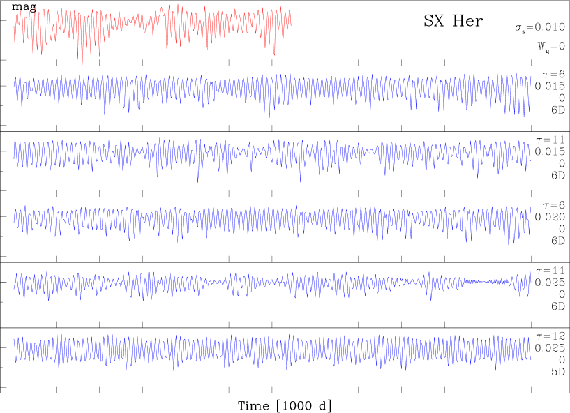
Figure 12.— SX Her: top: smoothed LC (mag); below: sections of synthetic LCs with various seeds and delays $\tau$ for maps constructed from the smoothed magnitude data; ($\tau$,$\sigma_{s}$,$W_{g}$) are indicated on the right ($W_{g}=0$ stands for no Gaussian filter);

SX Her: Fourier amplitude spectrum top: of the smoothed LC, below: of synthetic LCs. BK projections, top: smoothed LC, below: sections of synthetic LCs with various smoothings and delays $\tau$.

4.2. RS Cyg

In Figure 7 on top we display the 15 cycles long LC for RS Cyg, superposed on a LC fitted with the smoothings $\sigma_{s}=0.02$, $W_{g}=4$.

We find again that 3D reconstructions are not satisfactory at all, with the periods, in particular, being quite bad. The 4D reconstructions show some insensitivity to the smoothing, as long as it is large enough: Good LCs have been obtained from a range of typically 2 – 5 delay values which, depending on the amount of smoothing, range from $\tau=34$ to 40 d. Synthetic LC obtained from reconstructions with a smoothing of $\sigma_{s}=0.010$ and 0.020 were too regular, and the fixed points of the map are about 0.20 to 0.25 too large. The displayed synthetic LCs come from smoothing values $\sigma_{s}=0.025-0.04$. Typically there are from 2 to 6 $\tau$ values for which there are good synthetic LCs. Fig. 7 displays a sample of our best 12000 d long segments of 4D. This suggests that the embedding dimension for RS Cyg is also $d_{e}=4$. This conclusion is corroborated by the amplitude FS of Fig. 10 and the BK projections in Fig. 10.

The linear stability eigenvalues of the fixed points of the maps are shown in Table 2. The frequency ratios are approximately to 2:1 for the reconstructions with the larger values of $\sigma_{s}\geq 0.30$ that we have used. The growth rate $\kappa_{1}$ of the first mode is again positive (unstable) and that of the second mode $\kappa_{2}<0$, but not for $\sigma_{s}=0.025$. In all cases, the lowest frequency $f_{1}$ is reasonably close to the frequency of the fundamental peak in Fig. 10. That the linear stability eigenvalues of the fixed points are not very consistent is not very astonishing, because after all the amplitude of the LC is never small, and therefore it does not at all explore the neighborhood of the fixed point where the stability properties are determined.

The Lyapunov dimensions $d_{L}$ of all our good synthetic LCs are found to run from 2.1 to 3.2 with an average of $\sim 2.45$. The same average $d_{L}$ is obtained for the best few. This imposes a lower limit of 3 or 4 on $d$, but the latter can still be, and we believe it to be 4 for the same reasons we have given in the discussion on R UMi above. There are unfortunately too few data points to attempt a reconstruction in 5D which could corroborate that $d_{e}=4$.

We conclude that the analysis of the RS Cyg LC is consistent with, and perhaps suggests again that two interacting, highly nonadiabatic modes are at work, which in addition are in resonance. In other words RS Cyg seems to have the same underlying 4D dynamics that we have found for R Sct and R UMi.

4.3. V CVn

The smoothed V CVn LC is displayed in Fig. 9 ($\sigma_{s}=0.01$, $W_{g}=12$).

We have not been able to make any satisfactory 3D reconstructions for V CVn. However, the 4D reconstructions show insensitivity to the smoothing. For each smoothing set, good synthetic LCs have been obtained for typically 2 – 8 delay values which, depending on the amount of smoothing, range from $\tau=17$ to 27 d. Based on the visual appearance of the synthetic LCs the 4D reconstructions in Fig. 9 are good, suggesting $d_{e}=4$. However, for some reason, the dominant frequencies of all the synthetic LCs are systematically smaller  (Fig. 11), and the overtone frequencies are somewhat larger.

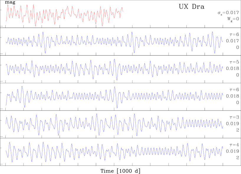
Figure 13.— UX Dra: top: smoothed LC (mag); below: sections of synthetic LCs with various seeds and delays $\tau$ for maps constructed from the smoothed magnitude data; ($\tau$,$\sigma_{s}$,$W_{g}$) are indicated on the right ($W_{g}=0$ stands for no Gaussian filter);

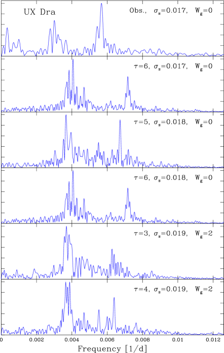
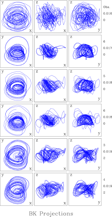
Figure 14.— UX Dra: amplitude FS, top: of the smoothed LC, below: of synthetic LCs. BK projections, top: of the smoothed LC, below: of synthetic LCs.

The BK projections, displayed in Fig. 11, are a little tamer for the synthetic LCs. The same difference is already apparent in Fig. 9, where the LCs show fluctuations in the average magnitude that are stronger than those of any of the synthetic ones. It could be that these fluctuations of the average magnitude are due to dust, or it could be that the dynamics is more complicated in the sense that a higher dimensional phase space (more modes) is required to capture it. In order to answer that question we would likely need a longer LC.

The Lyapunov dimensions $d_{L}$ of the good 4D synthetic LCs range from 3.4 to 3.6, substantially larger than for R UMi and RS Cyg. Good 5D reconstructions are also possible, but they occur only for one or 2 $\tau$ values that run from 15 to 26 d, depending on the smoothing. Significantly, the fractal dimensions of the good synthetic LCs run from $d_{L}=3.65$ to 4.02, i.e., they do not increase with $d_{R}$, corroborating that indeed $d_{e}=4$.

Another interesting difference with R Sct or R UMi appears in the linear stability eigenvalues of the fixed point displayed in Table 1. The frequencies associated with the linear stability eigenvalues of the fixed point are again in a close resonance ratio of 2:1, and the modes are highly nonadiabatic. However, here it is the higher frequency mode that is unstable, and the lower one that is stable.

In the study of Buchler et al. 2001 reconstructions were unsuccessful because the range of smoothing parameters was very limited. This shows that a survey with a range of smoothings is important.

4.4. SX Her

The smoothed LC of SX Her is shown on top of Fig. 12 with ($\sigma_{s}=0.01$, $W_{g}=0$). Underneath, are our best segments of synthetic LCs in several reconstruction dimensions $d_{R}$.

As for the previous stars, for SX Her the 3D reconstructions are not good at all. In 4D they are a little better, but still not very satisfactory, having more symmetry than the LC. As already found in Buchler et al. (2002) they are very sparse in $\tau$ space, and hence not robust. 5D reconstructions, while capturing some of the features of the LCs appear unsatisfactory. On the other hand, in 6D the synthetic LCs display many of the characteristic features of the LC, such as asymmetric bursts.

The Fourier spectra are shown in Fig. 4.1 for the same LCs displayed in Fig. 12. The first frequency is recovered relatively well, although the fundamental peak shows more structure than for the LC. The BK projections shown in Fig. 4.1 are reasonably good, but they reflect the tamer nature of the LCs and their smaller amplitudes.

We conclude that the dynamics which underlies the pulsations of SX Her may be more complicated than that of the other stars (to witness, for example, the intermittency in the central part of the analyzed LC) and therefore higher dimensional ($d>4$, perhaps $d=6$). However, this conclusion should be taken with some caution because the observational coverage of the LC is sparse in some places for this shorter ’period’ star, as Fig. 1 shows. It is also possible that we have missed a range of smoothing parameters where the lower-D reconstructions are successful.

4.5. UX Dra

Figure 13 on top displays a smoothed fit to the LC for UX Dra  ($\sigma_{s}=0.017$, $W_{g}=0$).

In a 3D reconstruction space the synthetic LCs definitely do not look like the LC. In 4D good looking synthetic LCs can be generated, although the reconstructions are not particularly robust. They appear possible only for a relatively narrow range of $\sigma_{s}$ and only for a few $\tau$ values in the range 3 – 6 d. This relative lack of robustness is not very astonishing considering that, compared to its complexity, the LC is very short. For a good reconstruction we clearly need LC features to repeat over the span of the LC. In addition the amplitude of this star is only half that of the other 4 stars, so that the noise level is higher. For the same reasons we have had difficulty making reconstructions in 5D and 6D. However, the synthetic LCs are consistent with $d_{e}=4$.

Figure 13 displays a sample of our best segments of 4D ynthetic LCs. The dominant frequencies of all the synthetic LCs are not very good as seen in the amplitude FS in Fig. 14. The BK projections of the synthetic LCs, although they bear a good resemblance to that of the LC, but are tamer. The Lyapunov dimensions for the synthetic LCs of Fig. 13 range from 2.4 to 3.1.

The linear stability analysis, shown in the Table 1, as for V CVn yields a stable low frequency, $f_{1}$, mode and an unstable $f_{2}$ mode, the stability being the reverse of that of R Sct and R UMi, but the same as for V CVn. However, the $f_{1}$ frequencies are not particularly close to the low frequency peak $\sim 0.003$ d^-1 in the FS, and the frequency ratio has a larger scatter around 2:1 than for the other stars.

We are forced to conclude that, either the observed LC of UX Dra are too short to make robust reconstructions, or perhaps the dynamics could be contaminated by dust formation and obscuration.

4.6. Discussion

In our survey we have only varied the dimension $d_{R}$, the smoothing parameters $\sigma_{s}$ and $W_{g}$ and the delays $\tau$. The polynomial order has been fixed at $p=4$. For the binning and averaging time interval we have chosen $\Delta t=10$d for all stars except UX Dra, where we obtained better results with $\Delta t=1$d. In general, we have not attempted to optimize the values of $\Delta t$ which might lead to more robust reconstructions.

Each vector component of our polynomial maps in 4D contains 70 coefficients, and one might be inclined object that it is not astonishing that such a map fits the data well, and that one would obtain an equally good fit with a (linear) multi-periodic Fourier sum with the same number of coefficients. However, for the latter is just a fit with limited predictive power and which tells us very little about the actual dynamics. In contrast, the constructed (nonlinear) maps have remarkable predictive power, i.e., the long synthetic LCs that we generate from the map do capture the dynamics as our comparisons have shown.

4.7. Comparison with the classical variable stars

The reader may be curious why in contrast to the Cepheids, which are the close relatives of the semiregular variables, pulsate in a regular, i.e., periodic or multiperiodic fashion. The fundamental physical difference is in the size of the relative linear growth rates (i.e., the growth rates $\times$ periods). For the classical variable stars, the latter are very small, of the order of a percent, whereas those of the Population II Cepheids, semiregulars and Mira variables are of order unity. The reason for this difference lies in the fact that the luminosity/mass ratio of the latter is about ten times larger. This causes a large increase in the coupling between pulsation and heat flow and concomitantly in the growth rates.

When the relative growth rates of the excited modes are small, as in the classical Cepheids, there exists near center manifold in the parlance of nonlinear dynamics, e.g., Buchler 1993). It can then be shown that the most complicated motions will be periodic pulsations (limit cycles) or multiperiodic pulsations (e.g., beat Cepheids).

No such manifold exists in the highly nonadiabatic semiregular stars, and more complicated, irregular (chaotic) pulsations can arise. Intuitively, large growth rates are a prerequisite for irregular pulsations, i.e., for amplitude modulation on the time scale of a period, although this is not sufficient.

It was shown unambiguously that the Hertzsprung progression of the Fourier phases of the bump Cepheids has its origin in a 2:1 resonance between the linearly unstable fundamental mode and the linearly stable second overtone (Buchler 1993). It is again the presence of a center manifold that gives rise to a synchronization of the two modes, and a periodic pulsation results in which the presence of the entrained second mode merely gives rise to a bump on the light curve. In contrast, although the same 2:1 resonance occurs in the Semiregulars, the absence of a center manifold allows the pulsation to be chaotic.

5. CONCLUSIONS

We have analyzed the 6500 day long observed LCs of the semiregular/Mira stars R UMi, V CVn, RS Cyg, SX Her and UX Dra. First, with a time-frequency analysis we have shown that in each case the dominant instantaneous frequency peak is not steady, and that the ’harmonic peak’ does not vary synchronously with the dominant one. This has led to the conclusion that these stars are not multi-periodic in the usual sense of the word, but that they are more likely to be generated by a low dimensional chaotic dynamics that involves a small number of pulsations modes. Multimode might therefore be a more suitable label for these stars than multiperiodic.

While a purely mathematical analysis might lead one to a stochastic nature of these pulsations, we have clearly ruled this out on physical grounds.

The results of a global flow reconstruction technique give strong evidence that the LCs of all five stars are generated by a low dimensional chaotic pulsation dynamics. The observed LCs of all 5 stars are really very short in terms of the number of pulsation cycles and their complexity, and our results must be taken with a little caution. However, interestingly, the evidence is very strong that for R UMi, RS Cyg and V CVn, and probably for UX Dra as well, the pulsation takes place in a 4D phase space. The LC of SX Her appears to be more complicated and perhaps a higher dimensional space, 6D, may be required.

Our analysis shows that the LCs of R Umi and RSC Cyg are generated by nonlinear dynamics that involve two resonant pulsation modes, a linearly self-excited lower frequency mode which entrains a second, linearly stable mode through a 2:1 resonance. The irregular pulsation occurs as a result of continual exchange of energy between the two resonant modes. This is the same scenario as was found for the irregularly pulsating RV Tau-type star R Sct (Buchler et al. 1995, 1996), but we caution that the reconstructions are not as robust as they are for R Sct because of the shortness of the observed light curves. In particular, we were not able to construct long synthetic LCs and extract a reliable Lyapunov dimension from these as for R Sct. The analysis of RS Cyg strongly suggests the presence of the same pulsation mechanism is operative.

Interestingly, the analysis shows that the LC of V CVn may similarly be due to a resonant interaction of two pulsation modes in a 2:1 resonance, but here it appears that the higher frequency mode is self-excited, whereas the lower frequency mode is stable. The analysis of UX Dra is much less conclusive, but is compatible with the same resonant 2-mode scenario.

To summarize then, we find good evidence for a common physical explanation for the irregularity that characterizes the pulsations of R UMi, RS Cyg, V CVn (and probably UX Dra) as we had found earlier for R Sct, namely that the underlying low dimensional chaotic pulsation dynamics arises from the nonlinear interaction of two resonant modes, and their high nonadiabaticity causes the pulsations to be chaotic.

- (1) Abarbanel, H.D.I., Brown, R., Sidorowich, J. J., Tsimring, L. S. 1993, RMP 65, 1331.
- (2) Ambika, G., Takeuti, M, Kembhavi, A.K., ASSL 283, 95.
- (3) Bergé, P., Pomeau, Y. & Vidal, C. 1986, Order Within Chaos (N.Y. : Wiley)
- (4) Boyle, R.P., Aspin, C., Coyne, G.V., McLean, I.S. 1986, A&A 164, 310
- (5) Broomhead, D. S. & King, G. P. 1987, Physica D 20, 217
- (6) Buchler, J. R. 1993, in Nonlinear Phenomena in Stellar Variability, Eds. M. Takeuti & J.R. Buchler (Kluwer: Dordrecht), repr. from ApSS 210, 1
- (7) Buchler, J. R. 1997, in International School of Physics “Enrico Fermi”, Course CXXXIII, Past and Present Variability of the Solar-Terrestrial System: Measurement, Data Analysis and Theoretical Models, Eds. G. Cini Castagnoli & A. Provenzale, Societa Italiana de Fisica, Bologna, Italy. p. 275
- (8) Buchler, J.R., Goupil M.J., Kovács G. 1993, AA 280, 157
- (9) Buchler, J.R., Goupil M.J., Kovács G. 1987, Phys Lett A 126, 177
- (10) Buchler, J. R. & Kovács, G. 1987, ApJLett, 320, L57
- (11) Buchler, J. R. & Kolláth, Z., 2001, Nonlinear Analysis of Irregular Variables, in Stellar Pulsation: Nonlinear Studies, Eds. M. Takeuti & D.D. Sasselov, ASSL Ser. 257, 185
- (12) Buchler J. R. & Kolláth, Z., 2003 Nonlinear Properties of the Semiregular Variable Stars in Mass-losing Pulsating Stars and Their Circumstellar Matter, ed. Y.Nakada, M.Honma & M. Seki, ASSL 283, 59.
- (13) Buchler, J. R., Kolláth, Z., Cadmus, R. R., Jr.2001, Chaos in the Music of the Spheres, Proceedings of CHAOS 2001, Potsdam, Germany, AIP Conf Proc 622, p. 61;
- (14) Buchler J. R., Kolláth, Z., Serre, T., Mattei, J. 1996, A&A 311, 833
- (15) Buchler, J.R. & Kovács, G. 1987, ApJ Lett 320, L57
- (16) Buchler, J. R., Serre, T., Kolláth, Z., Mattei, J. 1995, Phys Rev Lett 74, 842
- (17) Carney. B.W., Latham, D.W., Stefanik, R.P., Morse, J.A. 2003, AJ 125, 293
- (18) Cohen, L. 1994, Time-Frequency Analysis. Prentice-Hall PTR. Englewood Cliffs, NJ
- (19) Glendenning, P. & Tresser, C. 1985, J. Physique Lett. 46, L347
- (20) Gouesbet, G., LeSceller, L., Letellier, C., Brown, R., Buchler, J.R., Kolláth, Z. 1997, in Nonlinear Signal and Image Analysis, Ann. NY Acad. Sci. 808, p. 25
- (21) Hegger, R., Kantz, H., Schreiber, T. 1999, Chaos 9, 413
- (22) Kiss, L.L., Szatmáry, K. 2002, A&A 390, 585
- (23) Kiss, L.L., Szatmáry, K., Cadmus, R.R., Jr., Mattei, J.A. 1999, A&A 346, 542
- (24) Kiss, L.L., Szatmáry, K., Szabó, G., Mattei, J.A. 2000, A&AS 145, 283
- (25) Kolláth Z. 1990, MNRAS, 247, 377.
- (26) Kolláth, Z., Buchler, J. R., Szabó, R.& Csubry, Z. 2002, A&A 385, 932
- (27) Konig, M., Paunzen, E., Timmer,J. 1999, MNRAS 330, 297
- (28) Kovács, G. & Buchler, J. R. 1988, ApJ, 334, 971
- (29) Letellier, C., Gouesbet, G., Soufi, F., Buchler, J.R., Kolláth, Z., 1996, Chaos, 6, 466
- (30) Loeser, J.G., Baliunas, S.L., Guinan, E.F., Mattei, J.A., Wacker, S. 1986, in Cool Stars, Stellar Systems and the Sun, Proceedings of the Fourth Cambridge Workshop on Cool Stars, Stellar Systems, and the Sun, Zeilik, M. & Gibson, D.M., eds. (Springer-Verlag, New York), p.460
- (31) Magalhaes, A.M., Coyne, G.V., Benedetti, E.K. 1986, AJ 91, 919
- (32) Ott, E. 1993, Chaos in Dynamical Systems (Cambridge Univ. Press)
- (33) Percy, J.R. & Kolin, D.L. 2000, JAAVSO 28, 1
- (34) Preston G.W. & Wallerstein, G. 1963 ApJ 138, 820
- (35) Reinsch, C. H. 1967, Numerische Math, 10, 177
- (36) Serre, T., Kolláth, Z., Buchler, J. R. 1996, A&A 311:833–844
- (37) Weigend, A.S & Gershenfeld, N. A. 1994, Time Series Prediction (Addison-Wesley: Reading).
- (38) Zhao, Y., Atlas, L.E. & Marks, R.J. 1990, IEEE-ASSP 38, 1084