On Cross-correlating Weak Lensing Surveys

Abstract

The present generation of weak lensing surveys will be superseded by surveys run from space with much better sky coverage and high level of signal to noise ratio, such as SNAP. However, removal of any systematics or noise will remain a major cause of concern for any weak lensing survey. One of the best ways of spotting any undetected source of systematic noise is to compare surveys which probe the same part of the sky. In this paper we study various measures which are useful in cross correlating weak lensing surveys with diverse survey strategies. Using two different statistics - the shear components and the aperture mass - we construct a class of estimators which encode such cross-correlations. These techniques will also be useful in studies where the entire source population from a specific survey can be divided into various redshift bins to study cross correlations among them. We perform a detailed study of the angular size dependence and redshift dependence of these observables and of their sensitivity to the background cosmology. We find that one-point and two-point statistics provide complementary tools which allow one to constrain cosmological parameters and to obtain a simple estimate of the noise of the survey.

1 Introduction

Detection of weak lensing signals by observational teams (e.g., Bacon, Refregier & Ellis, 2000, Hoekstra et al., 2002, Van Waerbeke et al., 2000, and Van Waerbeke et al., 2002) has led to a new avenue not only in constraining the background dynamics of the universe but in probing the nature of dark matter and dark energy as well. To do so one compares observations with theoretical results obtained from simulations or analytical methods.

Numerical simulations of weak lensing typically employ ray-tracing techniques as well as line of sight integration of cosmic shear (e.g., Schneider & Weiss, 1988, Jarosszn’ski et al., 1990, Wambsganns, Cen & Ostriker, 1998, Van Waerbeke, Bernardeau & Mellier, 1999, and Jain, Seljak & White, 2000,Couchman, Barber & Thomas (1999)) and provide valuable insights.

On the other hand, analytical techniques to study weak lensing include perturbative calculations at large angular scales (e.g., Villumsen, 1996, Stebbins, 1996, Bernardeau et al., 1997, Jain & Seljak, 1997, Kaiser, 1998, Van Waerbeke, Bernardeau & Mellier, 1999, and Schneider et al., 1998) and techniques based on the hierarchical ansatz at small angular scales (e.g., Fry 1984, Schaeffer 1984, Bernardeau & Schaeffer 1992, Szapudi & Szalay 1993, 1997, Munshi, Melott & Coles 1999). Ingredients for such calculations include Peacock & Dodds (1996)’s prescription (see Peacock & Smith (2000) for a more recent fit) for the evolution of the power spectrum or equivalently the two-point correlation function. Recent studies have shown an excellent agreement between analytical results and numerical simulations of weak lensing effects (Valageas 2000a & b; Munshi & Jain 2000 & 2001; Munshi 2000; Bernardeau & Valageas 2000; Valageas, Barber & Munshi 2004; Barber, Munshi & Valageas 2004; Munshi, Valageas & Barber 2004).

However, to the weak lensing effects themselves one must add various sources of noise, such as the intrinsic ellipticity distribution of galaxies, shot-noise due to the discreet nature of the source galaxies and finite volume effects due to finite survey size. There is a need to incorporate all these in a consistent and systematic way in any realistic design of survey strategy. A detailed formalism to tackle such issues was developed by Munshi & Coles (2002) following Schneider et al. (1998). Recently Valageas, Munshi & Barber (2004) have used such techniques and have incorporated the redshift distribution of sources to model errors in future surveys such as SNAP.

In the near future we expect to see many weak lensing surveys probing overlapping areas of the sky with different survey strategies. These ground based observations will finally be superseded by surveys run from space with much better sky coverage such as SNAP. Nevertheless, removal of systematics and control of the noise from individual surveys will remain a major cause of concern. It is therefore of utmost importance that any undetected systematics be spotted by comparing different surveys which probe the same regions of the sky. Such a cross comparison will finally lead to the construction of large maps by combining smaller maps in an optimum way.

In our present study we focus on cross correlations among various surveys or different redshift bins in the same survey, with partial or complete overlap on their sky coverage. Using two different classes of statistics such as the smoothed shear components and the aperture mass, we construct estimators which encode such correlations. Based on analytical results from Munshi & Coles (2002) we generalize a recent study by Valageas, Munshi & Barber (2004) to take into account multiple surveys. We display the power of such techniques using SNAP class surveys where the source population can be subdivided into various redshift bins to study cross correlation among subsamples. We study the angular size dependence and redshift dependence of these classes of statistics. We also describe the dependence on background cosmological parameters.

This paper is organized as follows: in section 2, we describe our notations regarding weak lensing observables in general and various filters used to smooth the data. In section 3, we introduce weak lensing estimators which take into account various realistic sources of noise. Specific survey geometries based on SNAP class experiments are introduced in section 4 and we compute the noisy cumulant correlators of the aperture mass and of the shear components. Section 5 is devoted to a discussion of our results.

2 Notations and Formalism

Let us first recall our notations. Weak-lensing effects can be expressed in terms of the convergence along the line-of-sight towards the direction ${\vec{\vartheta}}$ on the sky up to the redshift $z_{s}$ of the source, $\kappa({\vec{\vartheta}},z_{s})$, given by (e.g., Bernardeau et al. 1997; Kaiser 1998):

$$\kappa({\vec{\vartheta}},z_{s})=\frac{3\Omega_{\rm m}}{2}\int_{0}^{\chi_{s}}{\rm d}\chi\;w(\chi,\chi_{s})\;\delta(\chi,{\cal D}{\vec{\vartheta}}),\;\;\;\mbox{with}\;\;\;w(\chi,\chi_{s})=\frac{H_{0}^{2}}{c^{2}}\;\frac{{\cal D}(\chi){\cal D}(\chi_{s}-\chi)}{{\cal D}(\chi_{s})}\;(1+z),$$ (1)

where $z$ corresponds to the radial distance $\chi$ and ${\cal D}$ is the angular distance. Here and in the following we use the Born approximation which is well-suited to weak-lensing studies: the fluctuations of the gravitational potential are computed along the unperturbed trajectory of the photon (Kaiser 1992). Thus the convergence $\kappa({\vec{\vartheta}},z_{s})$ is merely the projection of the local density contrast $\delta$ along the line-of-sight. Therefore, weak lensing observations allow us to measure the projected density field $\kappa$ on the sky (note that by looking at sources located at different redshifts one may also probe the radial direction). In practice the sources have a broad redshift distribution which needs to be taken into account. Thus, the quantity of interest is actually:

$$\kappa({\vec{\vartheta}})=\int_{0}^{\infty}{\rm d}z_{s}\;n(z_{s})\kappa({\vec{\vartheta}},z_{s}),\;\;\;\mbox{with}\;\int{\rm d}z_{s}\;n(z_{s})=1,$$ (2)

where $n(z_{s})$ is the mean redshift distribution of the sources (e.g. galaxies) normalized to unity. From eq.(1), the convergence $\kappa$ associated with a specific survey also reads:

$$\kappa({\vec{\vartheta}})=\int_{0}^{\chi_{\rm max}}{\rm d}\chi\;\tilde{w}(\chi)\;\delta(\chi,{\cal D}{\vec{\vartheta}}),\;\;\;\mbox{with}\;\tilde{w}(\chi)=\frac{3\Omega_{\rm m}}{2}\int_{z}^{z_{\rm max}}{\rm d}z_{s}\;n(z_{s})\;w(\chi,\chi_{s}),$$ (3)

where $z_{\rm max}$ is the depth of the survey (i.e. $n(z_{s})=0$ for $z_{s}>z_{\rm max}$). By working with eq.(3) we neglect the discrete effects due to the finite number of galaxies. They can be obtained by taking into account the discrete nature of the distribution $n(z_{s})$. This gives corrections of order $1/N$ to higher-order moments of weak-lensing observables, where $N$ is the number of galaxies within the circular field of interest. In practice $N$ is much larger than unity (for a circular window of radius 1 arcmin we expect $N\ga 100$ for the SNAP mission) therefore in this paper we shall work with eq.(3).

Thus, in order to take into account the redshift distribution of sources we simply need to replace $3\Omega_{\rm m}/2w(\chi,\chi_{s})$ in eq.(1) by $\tilde{w}(\chi)$. Therefore, all the results of Munshi et al. (2004) remain valid. Then, usual weak-lensing observables can be written as the angular average of $\kappa({\vec{\vartheta}})$ with some filter $U$:

$$X=\int{\rm d}{\vec{\vartheta}}\;U_{X}({\vec{\vartheta}})\;\kappa({\vec{\vartheta}}).$$ (4)

For instance, the filters associated with the smoothed convergence $\kappa_{s}$, the smoothed shear $\gamma_{s}$ and the aperture-mass $M_{\rm ap}$ are (Munshi et al. 2004):

$$U_{\kappa_{s}}=\frac{\Theta(\vartheta<\theta_{s})}{\pi\theta_{s}^{2}},\;\;\;U_{\gamma_{s}}=-\frac{\Theta(\vartheta>\theta_{s})}{\pi\vartheta^{2}}\;e^{i2\alpha}\;\;\;\mbox{and}\;\;\;U_{M_{\rm ap}}=\frac{\Theta(\vartheta<\theta_{s})}{\pi\theta_{s}^{2}}\;9\left(1-\frac{\vartheta^{2}}{\theta_{s}^{2}}\right)\left(\frac{1}{3}-\frac{\vartheta^{2}}{\theta_{s}^{2}}\right),$$ (5)

where $\Theta$ are Heaviside functions with obvious notations and $\alpha$ is the polar angle of the vector ${\vec{\vartheta}}$. The angular radius $\theta_{s}$ gives the angular scale probed by these smoothed observables. Note that the smoothed shear $\gamma_{s}$ depends on the matter located outside of the cone of radius $\theta_{s}$. However, in practice one directly measures the shear $\gamma({\vec{\vartheta}})$ on the direction ${\vec{\vartheta}}$ (from the ellipticity of a galaxy) rather than the convergence $\kappa$ and $\gamma_{s}$ is simply the mean shear within the radius $\theta_{s}$. For $M_{\rm ap}$ we shall use in this paper the filter (5), as in Schneider (1996), but one could also use any compensated filter with radial symmetry.

As described in Munshi et al. (2004), the cumulants of $X$ can be written as:

$$\langle X^{p}\rangle_{c}=\int_{0}^{\infty}\prod_{i=1}^{p}{\rm d}\chi_{i}\;\tilde{w}(\chi_{i})\int\prod_{j=1}^{p}{\rm d}{\vec{\vartheta}}_{j}\;U_{X}({\vec{\vartheta}}_{j})\;\;\xi_{p}\left(\begin{array}[]{l}\chi_{1}\\ {\cal D}_{1}{\vec{\vartheta}}_{1}\end{array},\begin{array}[]{l}\chi_{2}\\ {\cal D}_{2}{\vec{\vartheta}}_{2}\end{array},\dots,\begin{array}[]{l}\chi_{p}\\ {\cal D}_{p}{\vec{\vartheta}}_{p}\end{array}\right),$$ (6)

or equivalently we can write:

$$\langle X^{p}\rangle_{c}=\int_{0}^{\infty}\prod_{i=1}^{p}{\rm d}\chi_{i}\;\tilde{w}(\chi_{i})\int\prod_{j=1}^{p}{\rm d}{\bf k}_{j}\;W_{X}({\bf k}_{\perp j}{\cal D}_{j}\theta_{s})\;\;\left(\prod_{l=1}^{p}e^{ik_{\parallel l}\chi_{l}}\right)\;\;\langle\delta({\bf k}_{1})\dots\delta({\bf k}_{p})\rangle_{c}.$$ (7)

We note $\langle..\rangle$ the average over different realizations of the density field, $\xi_{p}$ is the real-space $p-$point correlation function of the density field $\xi_{p}({\bf x}_{1},..,{\bf x}_{p})=\langle\delta({\bf x}_{1})..\delta({\bf x}_{p})\rangle_{c}$, $k_{\parallel}$ is the component of ${\bf k}$ parallel to the line-of-sight, ${\bf k}_{\perp}$ is the two-dimensional vector formed by the components of ${\bf k}$ perpendicular to the line-of-sight and $W_{X}({\bf k}_{\perp}{\cal D}\theta_{s})$ is the Fourier transform of the window $U_{X}$:

$$W_{X}({\bf k}_{\perp}{\cal D}\theta_{s})=\int{\rm d}{\vec{\vartheta}}\;U_{X}({\vec{\vartheta}})\;e^{i{\bf k}_{\perp}.{\cal D}{\vec{\vartheta}}}.$$ (8)

In particular, for the smoothed convergence $\kappa_{s}$, the smoothed shear $\gamma_{s}$ and the aperture-mass $M_{\rm ap}$ we have (Munshi et al. 2004):

$$W_{\kappa_{s}}({\bf k}_{\perp}{\cal D}\theta_{s})=\frac{2J_{1}(k_{\perp}{\cal D}\theta_{s})}{k_{\perp}{\cal D}\theta_{s}},\;\;\;W_{\gamma_{s}}({\bf k}_{\perp}{\cal D}\theta_{s})=\frac{2J_{1}(k_{\perp}{\cal D}\theta_{s})}{k_{\perp}{\cal D}\theta_{s}}\;e^{i2\phi}\;\;\;\mbox{and}\;\;\;W_{M_{\rm ap}}({\bf k}_{\perp}{\cal D}\theta_{s})=\frac{24J_{4}(k_{\perp}{\cal D}\theta_{s})}{(k_{\perp}{\cal D}\theta_{s})^{2}},$$ (9)

where $\phi$ is the polar angle of ${\bf k}_{\perp}$ and $J_{\nu}$ are Bessel functions of the first kind. The real-space expression (6) is well-suited to models which give an analytic expression for the correlations $\xi_{p}$, like the minimal tree-model (Valageas 2000b; Bernardeau & Valageas 2002; Barber et al. 2004) while the Fourier-space expression (7) is convenient for models which give a simple expression for the correlations $\langle\delta({\bf k}_{1})..\delta({\bf k}_{p})\rangle_{c}$, like the stellar model (Valageas et al. 2004; Barber et al. 2004). In the present study we shall also be interested in two-point cumulants such as:

$$\langle X_{1}^{p}X_{2}^{q}\rangle_{c}=\int_{0}^{\infty}{\rm d}\chi\;(2\pi)^{p+q-1}\;\tilde{w}_{1}^{p}\tilde{w}_{2}^{q}\int\prod_{j=1}^{p+q}{\rm d}{\bf k}_{\perp j}\;W_{X}({\bf k}_{\perp j}{\cal D}\theta_{s})\;\langle\delta({\bf k}_{\perp 1})\dots\delta({\bf k}_{\perp p+q})\rangle_{c},$$ (10)

which describe the cross-correlations between two surveys or subsamples. Here the subscripts “1,2” refer to the two surveys we cross-correlate. In eq.(10) we used the fact that the correlation length is much smaller than cosmological scales and the Dirac factor $\delta_{D}(k_{\parallel 1}+\dots+k_{\parallel p+q})$ has been factorized out of $\langle\delta({\bf k}_{\perp 1})\dots\delta({\bf k}_{\perp p+q})\rangle_{c}$. The two-point correlators are similar to projected cumulant correlators studied in previous works (Szapudi & Szalay 1993; Munshi et al. 1999 ). However, unlike those projected cumulant correlators these objects are defined here in the zero angular separation limit where only the projection along the radial direction is different for the two surveys. Note that for observables like the aperture-mass which are very localized (long wavelengths are damped by the compensated filter) it is expected that projected cumulant correlators will only have non-negligible values if the angular separation is not much larger than the angular radius of the window.

From the one-point cumulants (6)-(7) it is convenient to define the parameters $S_{p}$ and the coefficients $t_{p}$:

$$S_{p}=\frac{\langle X^{p}\rangle_{c}}{\langle X^{2}\rangle_{c}^{p-1}},\hskip 28.45274ptt_{p}=\frac{\langle X_{1}^{p}\rangle_{c}}{\langle X_{2}^{p}\rangle_{c}}.$$ (11)

The quantities $S_{p}$ apply to one subsample while $t_{p}$ apply to two subsamples. The coefficients $S_{p}$ of weak lensing observables are closely related to the usual parameters $S_{p}$ which describe the departures of the underlying 3-d density field from Gaussianity (e.g., Valageas et al. 2004, Munshi et al. 2004). In particular, for the case of the smoothed convergence $\kappa_{s}$ we have $S_{p}^{{\hat{\kappa}}_{s}}\simeq S_{p}^{\delta}$ where ${\hat{\kappa}}_{s}$ is the smoothed convergence normalized by a suitable factor and $\delta$ is the 3-d density contrast (e.g., Barber et al. 2004). The normalization of the coefficients $S_{p}^{\delta}$ is such that they have a finite limit in the quasi-linear regime and show at most weak variations in the highly non-linear regime (but they exhibit a sharp change at the transition). Thus, from the one-point quantities $S_{p}$ we obtain the deviations from Gaussianity associated with each survey or subsample. Together with the second-order moments $\langle X^{2}\rangle$ (i.e. variance) they can be used to measure cosmological parameters as well as the non-Gaussianities built by the non-linear gravitational dynamics. In this regard, the redshift binning of the source population can also be very useful as it allows one to constrain the time evolution of cosmological distances and growth factors through the ratios $t_{p}$. Obviously, the weak lensing effects associated with different redshift bins are correlated since their lines of sight probe the same density fluctuations at low $z$ (where they are largest), for a fixed angular patch on the sky. In order to measure these cross-correlations we define the cross-correlation coefficients $r_{pq}$ as:

$$r_{pq}=\frac{\langle X_{1}^{p}X_{2}^{q}\rangle_{c}}{\langle X_{1}^{p+q}\rangle_{c}^{p/(p+q)}\langle X_{2}^{p+q}\rangle_{c}^{q/(p+q)}}\;,\;\;\;\mbox{in particular}\;\;\;r_{11}=\frac{\langle X_{1}X_{2}\rangle_{c}}{\langle X_{1}^{2}\rangle_{c}^{1/2}\langle X_{2}^{2}\rangle_{c}^{1/2}}.$$ (12)

The quantities $r_{pq}$ correspond to the two-point cumulants $\langle X_{1}^{p}X_{2}^{q}\rangle_{c}$ normalized in such a way that most of the dependence on cosmology and gravitational dynamics cancels out. Thus, if the two subsamples are highly correlated we have $r_{pq}\simeq 1$ while $r_{pq}\simeq 0$ if they are almost uncorrelated.

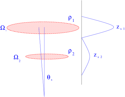
One often uses cumulant correlators to study the cross-correlations as a function of the separation angle $\theta_{12}$ between two different angular patches. In the numerical computations we perform in this paper we shall restrict ourselves to the case of zero angular separation. Hence we focus on the correlations between two surveys which overlap on the sky but which have different redshift distributions of sources (see Fig. 1). On the other hand, note that the signal would decrease for nonzero angular separations.

Figure 1: A schematic representation of cross-correlating two different source populations represented by mean source redshifts $z_{s1}$ and $z_{s2}$. Non-overlapping source distributions are considered. Survey areas are $\Omega_{1}$ and $\Omega_{2}$ respectively, the common smoothing angular radius is $\theta_{s}$. The contributions to the scatter of weak lensing estimators due to the galaxy intrinsic ellipticities of each sample can be described by the quantities $\rho_{1}(\theta_{s})$ and $\rho_{2}(\theta_{s})$ defined in eq.(16).

3 Low-order estimators and their scatter

The expressions obtained in the previous section describe weak lensing effects due to the fluctuations of the matter density field. However, in order to handle realistic data one needs to take into account the observational noise. A first source of scatter is due to the finite size of the surveys. A second source of noise is merely due to the intrinsic ellipticity of galaxies, which cannot be avoided. As in Munshi & Coles (2003) and Valageas, Munshi & Barber (2004), this leads us to define the estimators $M_{p}$ for low-order moments:

$$M_{p}=\frac{(\pi\theta_{s}^{2})^{p}}{(N)_{p}}\left[\sum_{(i_{1},\dots,i_{p})}^{N}Q_{i_{1}}\dots Q_{i_{p}}\;\epsilon_{i_{1}}\dots\epsilon_{i_{p}}\right],\;\;\;\mbox{with}\;\;\;(N)_{p}=N(N-1)..(N-p+1)=\frac{N!}{(N-p)!},$$ (13)

where $N$ is the number of galaxies in the patch of size $\pi\theta_{s}^{2}$ and $p$ is the order of the moment. Here we used the fact that the aperture-mass defined from the convergence $\kappa$ by the compensated filter $U_{M_{\rm ap}}$ given in eq.(5) can also be written as a function of the tangential shear $\gamma_{\rm t}$ as (Kaiser et al. 1994; Schneider 1996):

$$M_{\rm ap}=\int{\rm d}{\vec{\vartheta}}\;Q_{M_{\rm ap}}({\vec{\vartheta}})\;\gamma_{\rm t}({\vec{\vartheta}})\;\;\;\mbox{with}\;\;\;Q_{M_{\rm ap}}({\vec{\vartheta}})=\frac{\Theta(\vartheta<\theta_{s})}{\pi\theta_{s}^{2}}\;6\;\left(\frac{\vartheta}{\theta_{s}}\right)^{2}\left(1-\frac{\vartheta^{2}}{\theta_{s}^{2}}\right),$$ (14)

while for the smoothed shear components $\gamma_{i{\rm s}}$ (with $i=1,2$) we simply have:

$$\gamma_{i{\rm s}}=\int{\rm d}{\vec{\vartheta}}\;Q_{\gamma_{i{\rm s}}}({\vec{\vartheta}})\;\gamma_{i}({\vec{\vartheta}})\;\;\;\mbox{with}\;\;\;Q_{\gamma_{i{\rm s}}}({\vec{\vartheta}})=\frac{\Theta(\vartheta<\theta_{s})}{\pi\theta_{s}^{2}}.$$ (15)

Thus, in eq.(13) we wrote $Q_{j}=Q_{X}({\vec{\vartheta}}_{j})$ and we use the tangential ellipticity (for $M_{\rm ap}$) or the $i$-component of the ellipticity (for $\gamma_{i{\rm s}}$). Indeed, in the case of weak lensing, $\kappa\ll 1$, the observed complex ellipticity $\epsilon$ is related to the shear $\gamma$ by: $\epsilon=\gamma+\epsilon_{*}$, where $\epsilon_{*}$ is the intrinsic ellipticity of the galaxy. Finally, the sum in eq.(13) runs over all ordered sets of $p$ different galaxies among the $N$ galaxies enclosed in the angular radius $\theta_{s}$.

Then, neglecting any cross-correlations between the intrinsic ellipticities of different galaxies and between the matter density field and the galaxy intrinsic ellipticities, the estimators $M_{p}$ introduced in eq.(13) are unbiased estimators of low-order moments of the aperture-mass or of the shear components. Moreover, their dispersion $\sigma^{2}(M_{p})=\langle M_{p}^{2}\rangle-\langle M_{p}\rangle^{2}$ only involves the variance $\sigma_{*}^{2}=\langle|\epsilon_{*}|^{2}\rangle$ of the galaxy intrinsic ellipticities (even if the latter are not Gaussian). The latter enters the scatter $\sigma^{2}$ through the combination $\rho$ defined by:

$$\rho=\frac{2N\langle X^{2}\rangle}{\sigma_{*}^{2}G_{X}}\;\;\;\mbox{with}\;\;\;G_{X}=\pi\theta_{s}^{2}\int{\rm d}{\vec{\vartheta}}\;Q_{X}({\vec{\vartheta}})^{2},\;\;\;\mbox{whence}\;\;\;G_{M_{\rm ap}}=\frac{6}{5},\;\;\;G_{\gamma_{i{\rm s}}}=1.$$ (16)

Here $N$ is the number of galaxies within the circular field of angular radius $\theta_{s}$. The quantity $\rho$ measures the relative importance of the galaxy intrinsic ellipticities in the signal. They can be neglected if $\rho\gg 1$. Thus, the mean of the estimator $M_{2}$ and its scatter are given by (with $\langle X\rangle=0$, see also Valageas et al. 2004):

$$\langle M_{2}\rangle=\langle X^{2}\rangle_{c}\;\;\;\mbox{and}\;\;\;\sigma^{2}(M_{2})=\langle X^{4}\rangle_{c}+\langle X^{2}\rangle_{c}^{2}\;2\;\left[1+{1\over\rho}\right]^{2}.$$ (17)

In order to obtain eq.(17) we have averaged i) over the intrinsic ellipticity distribution, ii) over the galaxy positions and iii) over the matter density field, assuming these three averaging procedures are uncorrelated. Any Gaussian white noise associated with the detector can be incorporated into these expressions by adding a relevant correction to $\sigma_{*}^{2}$ (whence to $\rho$). Note that the scatter of low-order estimators involves higher-order cumulants (up to twice the order of the moment one wishes to evaluate). Here we have neglected the terms due to the finite number of galaxies which scale as $1/N$ and are negligible for practical purposes ($N\gg 1$). The dispersion $\sigma^{2}$ obtained in eq.(17) takes into account two sources of noise: the galaxy intrinsic ellipticities (the terms which depend on $\rho$) and the finite size of the survey (the remaining terms).

The estimators $M_{p}$ defined in eq.(13) correspond to a single circular field of angular radius $\theta_{s}$ containing $N$ galaxies. In practice, the size of the survey is much larger than $\theta_{s}$ and we can average over $N_{c}$ cells on the sky. This yields the estimators ${\cal M}_{p}$ defined by:

$${\cal M}_{p}=\frac{1}{N_{c}}\sum_{n=1}^{N_{c}}M_{p}^{(n)},\;\;\;\mbox{whence}\;\;\;\langle{\cal M}_{p}\rangle=\langle M_{p}\rangle=\langle X^{p}\rangle\;\;\;\mbox{and}\;\;\;\sigma({\cal M}_{p})=\frac{\sigma(M_{p})}{\sqrt{N_{c}}}\;\;\;\mbox{with}\;\;\;\sigma^{2}({\cal M}_{p})=\langle{\cal M}_{p}^{2}\rangle-\langle{\cal M}_{p}\rangle^{2},$$ (18)

where $M_{p}^{(n)}$ is the estimator $M_{p}$ for the cell $n$ and we assumed that these cells are sufficiently well separated so as to be uncorrelated.

The estimators $M_{p}$ and ${\cal M}_{p}$ provide a measure of the moments $\langle X^{p}\rangle$ of weak lensing observables, which can be used to evaluate the $S_{p}$ parameters defined in eq.(11). However, as shown in Valageas et al. (2004), it is better to first consider cumulant-inspired estimators $H_{p}$. Thus, for the aperture mass where we shall restrict ourselves to third-order cumulants we define:

$$H_{3}=M_{3}-3{\cal M}_{2}M_{1}\;\;\;\mbox{and}\;\;\;{\cal H}_{3}=\frac{1}{N_{c}}\sum_{n=1}^{N_{c}}H_{3}^{(n)},\;\;\;\mbox{whence}\;\;\;\langle{\cal H}_{3}\rangle=\langle M_{\rm ap}^{3}\rangle_{c},$$ (19)

while for the shear components which are even quantities (so that all odd-order moments vanish) we need to go up to fourth order and we define:

$$H_{4}=M_{4}-6{\cal M}_{2}M_{2}+3{\cal M}_{2}^{2}\;\;\;\mbox{and}\;\;\;{\cal H}_{4}=\frac{1}{N_{c}}\sum_{n=1}^{N_{c}}H_{4}^{(n)},\;\;\;\mbox{whence}\;\;\;\langle{\cal H}_{4}\rangle=\langle\gamma_{i{\rm s}}^{4}\rangle_{c}.$$ (20)

The interest of $H_{3}$ and $H_{4}$ is that their scatter is smaller than for $M_{3}$ and $M_{4}$, see Valageas et al. (2004). Besides they directly yield the one-point cumulants (here we neglected higher-order terms over $1/N_{c}$).

As for galaxy surveys (Szapudi & Szalay 1997) we can generalize the estimators (13) to measure the cross-correlations between two surveys (or two subsamples) by defining:

$$M_{pq}=\frac{(\pi\theta_{s1}^{2})^{p}(\pi\theta_{s2}^{2})^{q}}{(N_{1})_{p}(N_{2})_{q}}\left[\sum_{(i_{1},\dots,i_{p})}^{N_{1}}\sum_{(j_{1},\dots,j_{q})}^{N_{2}}Q_{i_{1}}\epsilon_{i_{1}}\dots Q_{i_{p}}\epsilon_{i_{p}}Q_{j_{1}}\epsilon_{j_{1}}\dots Q_{j_{q}}\epsilon_{j_{q}}\right].$$ (21)

Obviously, these estimators could be extended to $s-$point correlations between $s$ surveys. In this paper we shall only consider the case $\theta_{s1}=\theta_{s2}$. Then, as in eq.(18) we can define the estimators ${\cal M}_{pq}$ by averaging $M_{pq}$ over $N_{c}$ cells. Of course, the one-point estimators can also be written $M_{p}=M_{p0}$ or $M_{p}=M_{0p}$ depending on which survey they apply to. Next, we can define the analogs of the one-point estimators $H_{p}$ and ${\cal H}_{p}$. For the aperture mass, there is only one new cross-correlation at third order, $M_{21}$ (and its symmetric $M_{12}$), and we define:

$$H_{21}=M_{21}-2{\cal M}_{11}M_{10}-{\cal M}_{20}M_{01}\;\;\;\mbox{whence}\;\;\;\langle{\cal H}_{21}\rangle=\langle M_{\rm ap1}^{2}M_{\rm ap2}\rangle_{c}.$$ (22)

For the shear components $\gamma_{i{\rm s}}$ we have two new cross-correlations at fourth order, $M_{31}$ (and its symmetric $M_{13}$) and $M_{22}$, and we define:

$$H_{31}=M_{31}-3{\cal M}_{11}M_{20}-3{\cal M}_{20}M_{11}+3{\cal M}_{11}{\cal M}_{20},\;\;\mbox{whence}\;\;\langle{\cal H}_{31}\rangle=\langle\gamma_{i{\rm s}1}^{3}\gamma_{i{\rm s}2}\rangle_{c}=\langle\gamma_{i{\rm s}1}^{3}\gamma_{i{\rm s}2}\rangle-3\langle\gamma_{i{\rm s}1}^{2}\rangle\langle\gamma_{i{\rm s}1}\gamma_{i{\rm s}2}\rangle,$$ (23)

and:

$$H_{22}=M_{22}-{\cal M}_{20}M_{02}-{\cal M}_{02}M_{20}-4{\cal M}_{11}M_{11}+{\cal M}_{20}{\cal M}_{02}+2{\cal M}_{11}{\cal M}_{11},$$ (24)

whence:

$$\langle{\cal H}_{22}\rangle=\langle\gamma_{i{\rm s}1}^{2}\gamma_{i{\rm s}2}^{2}\rangle_{c}=\langle\gamma_{i{\rm s}1}^{2}\gamma_{i{\rm s}2}^{2}\rangle-\langle\gamma_{i{\rm s}1}^{2}\rangle\langle\gamma_{i{\rm s}2}^{2}\rangle-2\langle\gamma_{i{\rm s}1}\gamma_{i{\rm s}2}\rangle^{2}.$$ (25)

Again, one can easily check that the scatter of $H_{pq}$ is always smaller than the scatter of $M_{pq}$ (see Appendix). Finally, from these estimators ${\cal H}_{p}$ and ${\cal H}_{pq}$ we can evaluate the parameters $S_{p}$, $t_{p}$ and the cross-correlation coefficients $r_{pq}$ introduced in eqs.(11), (12), through the estimators ${\cal S}_{p}$, ${\cal T}_{p}$ and ${\cal R}_{pq}$:

$${\cal S}_{p}=\frac{{\cal H}_{p}}{{\cal M}_{2}^{p-1}},\hskip 28.45274pt{\cal T}_{p}=\frac{{\cal H}_{p0}}{{\cal H}_{0p}}\hskip 28.45274pt\mbox{and}\hskip 28.45274pt{\cal R}_{pq}=\frac{{\cal H}_{p,q}}{{\cal H}_{p+q,0}^{p/(p+q)}{\cal H}_{0,p+q}^{q/(p+q)}}.$$ (26)

We can note from numerical computations that the scatter of the moments $\langle X_{1}^{p}X_{2}^{q}\rangle$ increases very rapidly with the order $p+q$. Therefore, we can neglect the contributions to the scatter of ${\cal S}_{p}$ due to the denominator. Hence we write:

$$\langle{\cal S}_{p}\rangle\simeq S_{p},\hskip 14.22636pt\sigma({\cal S}_{p})\simeq\frac{\sigma({\cal H}_{p})}{\langle X^{2}\rangle^{p-1}},\hskip 14.22636pt\langle{\cal T}_{p}\rangle\simeq t_{p}\hskip 14.22636pt\mbox{and}\hskip 14.22636pt\langle{\cal R}_{pq}\rangle\simeq r_{pq},$$ (27)

$$\sigma^{2}({\cal T}_{p})\simeq t_{p}^{2}\left[\frac{\sigma^{2}({\cal H}_{p0})}{\langle X_{1}^{p}\rangle_{c}^{2}}+\frac{\sigma^{2}({\cal H}_{0p})}{\langle X_{2}^{p}\rangle_{c}^{2}}-2\frac{\sigma^{2}({\cal H}_{p0};{\cal H}_{0p})}{\langle X_{1}^{p}\rangle_{c}\langle X_{2}^{p}\rangle_{c}}\right],$$ (28)

and:

$$\sigma^{2}({\cal R}_{pq}) \simeq r_{pq}^{2}\Biggl{\{}\frac{\sigma^{2}({\cal H}_{p,q})}{\langle X_{1}^{p}X_{2}^{q}\rangle_{c}^{2}}+\left(\frac{p}{p+q}\right)^{2}\frac{\sigma^{2}({\cal H}_{p+q,0})}{\langle X_{1}^{p+q}\rangle_{c}^{2}}+\left(\frac{q}{p+q}\right)^{2}\frac{\sigma^{2}({\cal H}_{0,p+q})}{\langle X_{2}^{p+q}\rangle_{c}^{2}}-\frac{2p}{p+q}\frac{\sigma^{2}({\cal H}_{p,q};{\cal H}_{p+q,0})}{\langle X_{1}^{p}X_{2}^{q}\rangle_{c}\langle X_{1}^{p+q}\rangle_{c}}$$ (29)

$$-\frac{2q}{p+q}\frac{\sigma^{2}({\cal H}_{p,q};{\cal H}_{0,p+q})}{\langle X_{1}^{p}X_{2}^{q}\rangle_{c}\langle X_{2}^{p+q}\rangle_{c}}+\frac{2pq}{(p+q)^{2}}\frac{\sigma^{2}({\cal H}_{p+q,0};{\cal H}_{0,p+q})}{\langle X_{1}^{p+q}\rangle_{c}\langle X_{2}^{p+q}\rangle_{c}}\Biggl{\}}.$$

Here we assumed that the scatter of ${\cal T}_{p}$ and ${\cal R}_{pq}$ is small so that it can be linearized in eqs.(26). If this is not the case, that is $\sigma^{2}({\cal T}_{p})\ga 1$ or $\sigma^{2}({\cal R}_{pq})\ga 1$, the error-bar obtained from eq.(28) or eq.(29) is not correct (it significantly underestimates the scatter) but this means that the measure is dominated by the noise so that we do not need an accurate estimate of $\sigma^{2}$: we only wish to be aware that the noise is too large to allow a precise measure of $t_{p}$ or $r_{pq}$. In eqs.(28)-(29) we introduced the cross-dispersions $\sigma^{2}({\cal H}_{p,q};{\cal H}_{p^{\prime},q^{\prime}})$ defined by:

$$\sigma^{2}({\cal H}_{p,q};{\cal H}_{p^{\prime},q^{\prime}})=\langle{\cal H}_{p,q}{\cal H}_{p^{\prime},q^{\prime}}\rangle-\langle{\cal H}_{p,q}\rangle\langle{\cal H}_{p^{\prime},q^{\prime}}\rangle.$$ (30)

We give in appendix A the expression of the various dispersions $\sigma^{2}$ which we need in this article.

4 Numerical Results

In this section we numerically evaluate the signal to noise ratios involved with the various estimators described in the previous section. We assume a specific model for the background cosmology, a specific correlation hierarchy for the matter distribution and we focus on the SNAP observational strategy for numerical calculations. However as mentioned before the basic formalism developed here remains completely general and specific details studied here only serve illustrational purposes.

4.1 Cosmological Parameters

For the background cosmology we consider a fiducial LCDM model with $\Omega_{\rm m}=0.3$, $\Omega_{\Lambda}=0.7$, $H_{0}=70$ km/s/Mpc and $\sigma_{8}=0.88$. To check the sensitivity of cross-correlations on the background dynamics of the universe we shall also study the effect of small variations of these parameters onto weak-lensing observables and their cross-correlations. We consider many-body correlations of the matter density field which obey the stellar model (Valageas et al. 2004; Munshi et al. 2004). This is actually identical to the minimal tree-model up to third-order moments (Munshi et al. 2004). This is also coupled to the fit to the non-linear power-spectrum $P(k)$ of the dark matter density fluctuations given by Peacock & Dodds (1996). Lowest order non-Gaussian signatures will be at third order for $M_{\rm ap}$ and at fourth order for smoothed shear components $\gamma_{i{\rm s}}$.

4.2 Survey Parameters

Hereafter, we adopt the characteristics of the SNAP mission as given in Refregier et al.(2004). More precisely, we consider the “Wide” survey where the redshift distribution of galaxies is given by:

$$n(z_{s})\propto z_{s}^{2}\;e^{-(z_{s}/z_{0})^{2}}\;\;\;\mbox{and}\;\;\;z_{0}=1.13,\;\;\;z_{\rm max}=3.$$ (31)

The variance in shear due to intrinsic ellipticities and measurement errors is $\sigma_{*}=\langle|\epsilon_{*}|^{2}\rangle^{1/2}=0.31$. The survey covers an area $A=300$ deg² and the surface density of usable galaxies is $n_{g}=100$ arcmin^-2. Therefore, we take for the number $N$ of galaxies within a circular field of radius $\theta_{s}$:

$$N=n_{g}\pi\theta_{s}^{2}\simeq 314\left(\frac{n_{g}}{100\mbox{arcmin}^{-2}}\right)\left(\frac{\theta_{s}}{1\mbox{arcmin}}\right)^{2},$$ (32)

and for the number $N_{c}$ of cells of radius $\theta_{s}$:

$$N_{c}=\frac{A}{(2\theta_{s})^{2}}=2.7\times 10^{5}\left(\frac{A}{300\mbox{deg}^{2}}\right)\left(\frac{\theta_{s}}{1\mbox{arcmin}}\right)^{-2}.$$ (33)

For the shear this number somewhat overestimates $N_{c}$ because of the sensitivity of $\gamma_{i{\rm s}}$ to long wavelengths, which would require the centres of different cells to be separated by more than $2\theta_{s}$ in order to be uncorrelated.

In order to extract some information from the redshift dependence of weak lensing effects, which could also be used to discriminate noise sources, we also divide the “Wide” SNAP survey into two redshift bins. Then, we shall study the cross correlations between both bins. Thus, we consider the two subsamples which can be obtained from the “Wide” survey by dividing galaxies into two redshift bins: $z_{s}>z_{*}$ and $z_{s}<z_{*}$. We choose $z_{*}=1.23$, which corresponds roughly to the separation provided by the SNAP filters and which splits the “Wide” SNAP survey into two samples with the same number of galaxies (hence $n_{g}=50$ arcmin^-2). Note that one cannot use too many redshift bins at it decreases the number of source galaxies associated with each subsample (for the aperture mass we could still obtain good results with three bins but we shall restrict ourselves to two redshift bins in this paper). The redshift bins that we use are similar to those which are used by Refregier et al.(2003) using photometric redshifts, except that they have a sharp cutoff and non-overlapping source distributions. Note that using overlapping source distributions (over redshift) would increase the cross-correlations.

4.3 Numerical evaluation of Estimators and their scatter

For all our computations we use the matter correlation hierarchy introduced and tested in a recent series of papers for the evaluation of statistics related to shear and $M_{\rm ap}$ statistics. These analytical models were tested extensively against numerical simulations and were found to provide satisfactory results. We have studied the cross correlations among the two redshift bins obtained from the “Wide” SNAP survey using both the aperture mass $M_{\rm ap}$ and the smoothed shear components $\gamma_{i{\rm s}}$. In the following, in weak-lensing observables of the form $H_{pq}$ the first index $p$ refers to the low-$z$ subsample and the second index $q$ to the high-$z$ subsample.

4.3.1 Aperture mass statistics $M_{\rm ap}$

Second-order cumulants

Figure 2: Left panel shows the quantity $\rho(\theta_{s})$ which measures the relative importance of galaxy intrinsic ellipticities, for the aperture mass and two redshift bins, as a function of the angular scale $\theta_{s}$ (in arcmin). The variance $\langle M_{\rm ap}^{2}\rangle$ for these two redshift bins is displayed in middle (low-$z$ subsample) and right (high-$z$ subsample) panels. Various line styles correspond to various cosmological or survey parameters. The solid “$\Lambda$” line is our fiducial model described in sections 4.1-4.2. The dotted “$\Omega_{\rm m}$” curve shows the effect of a $10\%$ increase of $\Omega_{\rm m}$ (from $\Omega_{\rm m}=0.3$ up to $\Omega_{\rm m}=0.33$), the dot-dashed “$\sigma_{8}$” line corresponds to a $10\%$ increase of $\sigma_{8}$ (from $\sigma_{8}=0.88$ up to $\sigma_{8}=0.97$) while the dashed “$z_{0}$” curve represents a $10\%$ decrease of the characteristic redshift $z_{0}$ of the survey (from $z_{0}=1.13$ down to $z_{0}=1.02$). These line styles will be used in the following plots. The error bars show the one $\sigma$ dispersion around the mean value.

Figure 3: The quantities $t_{2}$ and $r_{11}$ (see text for description) for $M_{\rm ap}$ are plotted as a function of smoothing angle $\theta_{s}$ for the two redshift bins. Error bars correspond again to the one $\sigma$ dispersion around the mean value.

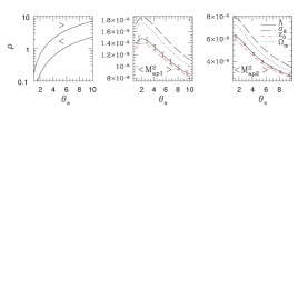
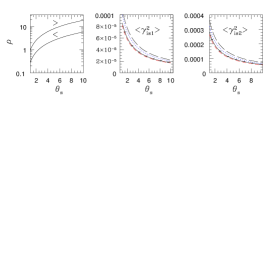
We first present in the left panel of Fig.2 the quantity $\rho(\theta_{s})$ as a function of the angular smoothing radius $\theta_{s}$ for the two redshift bins obtained from the “Wide” SNAP survey. We can note that $\rho$ is of order unity which means that the galaxy intrinsic ellipticities yield a significant contribution to the signal which cannot be neglected (but weak lensing effects can still be extracted). The relative importance of intrinsic ellipticities decreases at large scales ($\rho$ increases) as the number $N$ of galaxies within the angular radius $\theta_{s}$ grows (this effect dominates over the decrease of the amplitude of weak lensing distortions, see eq.(16)). The quantity $\rho$ is larger for the high-redshift subsample because its variance $\langle M_{\rm ap}^{2}\rangle_{c}$ is larger (see eq.(16)).

Next, we show in the middle and right panels of Fig.2 the variance $\langle M_{\rm ap}^{2}\rangle$ of the aperture mass for each redshift subsample. The four curves correspond to our fiducial LCDM model and to a $10\%$ variation of $\Omega_{\rm m}$, $\sigma_{8}$ or $z_{0}$. We can see that the error-bars are quite small and would allow an accurate measure of the cosmological parameters. However, the signal is also sensitive to the redshift distribution of the sources which may be an important limiting factor (although the dependence is rather weak). As is well known, the amplitude of weak lensing distortions increases with the redshift of the sources as the line of sight is longer, hence the variance is larger for the high-$z$ subsample. On the other hand, it decreases at larger angular scales where the amplitude of density fluctuations is smaller. Note that the error-bars for the variance are quite small which justifies the approximation (27) for the scatter of $S_{p}$.

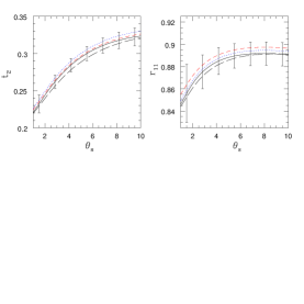
Then, we display in the left panel of Fig.3 the ratio $t_{2}$ between the variances $\langle M_{\rm ap}^{2}\rangle$ of the weak lensing effects associated with each redshift bin, as defined in eq.(11). In agreement with Fig.2 we have $t_{2}<1$. We can see that the sensitivity to cosmological parameters is rather modest. The error-bars are of the same order as the variation with a $10\%$ change of cosmological parameters so that by combining several angular scales one can get a useful constraint on cosmology. In particular, note that $\Omega_{\rm m}$ and $\sigma_{8}$ affect the ratio $t_{2}$ in opposite directions while they affect the variances $\langle M_{\rm ap}^{2}\rangle$ in the same direction. Thus, dividing weak lensing surveys like the SNAP mission into several redshift bins provides additional information in addition to the overall amplitude of weak lensing effects averaged over all source redshifts.

Finally, we present in the right panel of Fig.3 the cross-correlation coefficient $r_{11}$ (defined in eq.(12)) between the two redshift bins, for our four models. We can see that the cross-correlation is quite strong ($r_{11}\simeq 0.9$) with a small scatter. Indeed, the lines of sight associated with the two subsamples probe the same density fluctuations at low $z$, where they are largest because of the build-up of large-scale structures. Moreover, the cross-correlation coefficient $r_{11}$ only shows a very weak dependence on cosmology or the redshift distribution of sources: as the two subsamples are highly correlated most of the dependence on cosmology or source redshifts which appeared in Fig.2 cancels out between the numerator and denominator in eq.(12). This also leads to reasonably small error-bars since the dispersions of the numerator and denominator do not merely add up in quadrature, see eq.(29). The fact that the dependence on cosmology is very weak (and smaller than error-bars) means that the cross-correlation coefficient $r_{11}$ and the cross-product $\langle M_{\rm ap1}M_{\rm ap2}\rangle$ are not useful to constrain cosmological parameters. They do not add much information about cosmology to the one already included in the one-point statistics $\langle M_{\rm ap1}^{2}\rangle$ and $\langle M_{\rm ap2}^{2}\rangle$. However, we can take advantage of this property to use $r_{11}$ to measure the observational noise. Indeed, since $r_{11}$ can be predicted up to a very good accuracy (e.g. from other statistics like the one-point variance within the same survey, or from other sources like the CMB) its value gives a simple estimate of the scatter of second-order cumulants as measured in a specific survey. It could also help track down systematics. As noticed in section 3, eq.(29) for the scatter of the cross-correlation coefficient $r_{11}$ assumed that the dispersion was small $\sigma\ll 1$. If this is not the case, that is the value $r_{11}$ obtained from a weak-lensing survey shows a large departure from its theoretical mean (e.g., one measures $r_{11}\la 0.5$), then eq.(29) is an underestimate. Besides, the probability distribution of $r_{11}$ would be strongly non-Gaussian. Then, the estimate of the dispersion $\sigma$ of second-order cumulants one would derive from the measure of $r_{11}$ would be too large. Therefore, the break-up of eq.(29) in this domain is not a real problem since it merely yields conservative estimates for the noise (besides in such cases the data is too noisy to provide accurate constraints on cosmology).

Third-order cumulants

Figure 4: The skewness $S_{3}$ of the aperture mass is displayed as a function of the smoothing angle $\theta_{s}$, for the low-$z$ subsample (left panel) and the high-$z$ subsample (right panel).

Figure 5: The ratios $t_{3}$, $r_{21}$ and $r_{12}$, for the $M_{\rm ap}$ statistic and two redshift bins, are plotted in left, middle and right panel respectively. Error bars correspond again to one $\sigma$ scatter. Note the very weak dependence on cosmology or source redshift.

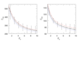
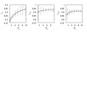
The variance of weak lensing observables cannot simultaneously constrain several cosmological parameters. Thus, in order to break the $\Omega_{\rm m}-\sigma_{8}$ degeneracy it was proposed to consider the skewness $S_{3}$ (Bernardeau et al. 1997). More generally, taking into account higher-order cumulants brings further information which can help constrain the underlying cosmology. However, the noise increases very rapidly with the order of the observed cumulants so that we shall restrict ourselves to the lowest-order non-vanishing cumulants beyond second-order. For the aperture mass this simply corresponds to third-order statistics like the skewness $S_{3}$ defined in eq.(11) (note that another possibility is to look at the whole probability distribution itself, see Valageas et al. 2004). We present in Fig.4 the skewness $S_{3}$ of the aperture mass as a function of the smoothing angle $\theta_{s}$ for the two redshift bins. In agreement with previous works we find that the skewness increases for lower source redshifts (because of the smaller length of the line of sight and of the growth with time of the non-Gaussianities of the density field). Hence we can check that $S_{30}>S_{03}$. We can see that although the scatter is much larger than for the variance, one should obtain a clear detection of non-Gaussianity in all cases. Moreover, by combining different angular scales and redshift bins (e.g. through a Fisher matrix approach) one should be able to constrain cosmological parameters at a $10\%$ level (note however the large dependence on the source redshift, which is more important than for second-order cumulants).

We present in the left panel of Fig.5 the ratio $t_{3}$ between the third-order weak-lensing cumulants associated with the two redshift bins. In agreement with Fig.4 we obtain $t_{3}<1$. We note that the dependence on cosmology is very small and much below error-bars. Therefore, redshift binning is not very useful to constrain cosmological parameters when it is applied to these third-order statistics. On the other hand, the measure of $t_{3}$ could be used to evaluate the noise of third-order cumulants (or the skewness) since its value can be predicted with a good accuracy (without requiring a high accuracy for cosmological parameters). This can be useful to assess the reliability of the data.

Next, we display in the middle and right panels of Fig.5 the cross-correlation coefficients $r_{21}$ and $r_{12}$ between both subsamples, as defined in eq.(12). We can check that the cross-correlation is very strong ($r\sim 0.9$) which means that the weak lensing effects associated with the two redshift bins are highly correlated. Of course, this is consistent with the high value already obtained for the cross-correlation $r_{11}$ of second-order cumulants (Fig.3). Note that we get $r_{21}>r_{12}>r_{11}$. Indeed, higher-order cumulants give more weight to the common low-$z$ parts of the line of sights (because the parameters $S_{p}$ of the 3-d density field increase in the non-linear regime). This increases the correlation of higher-order weak lensing cumulants. Similarly, the coefficient $r_{21}$ is slightly larger than $r_{12}$ as it gives more weight to low-$z$ distortions. We can note that the scatter of the cross-correlation coefficients $r_{21}$ and $r_{12}$ is somewhat smaller than might be guessed from the dispersion of third-order cumulants (Fig.4). This is again due to their high correlation. As for the second-order cross-correlation $r_{11}$, the dependence on cosmology or the source redshifts is very small (and much below error-bars). This means that $r_{21}$ and $r_{12}$, as the cross-products $\langle M_{\rm ap1}^{2}M_{\rm ap2}\rangle_{c}$ and $\langle M_{\rm ap1}M_{\rm ap2}^{2}\rangle_{c}$, do not bring additional information to the one-point cumulants $S_{3}$ with regard to cosmology. However, even though they are mostly useless with respect to the measure of cosmological parameters, they can be very useful to evaluate the noise of third-order cumulants. Indeed, a simple measure of $r_{21}$ or $r_{12}$ allows a good estimate of the noise of the skewness since their theoretical value can be predicted with a good accuracy. Therefore, cross-correlations are a complementary tool to one-point statistics and should prove useful.

4.3.2 Smoothed shear components $\gamma_{i{\rm s}}$

We now describe our results for the shear components, following the outline of our study of the aperture mass.

Second-order cumulants

Figure 6: Same as Fig.2 but for shear components. Left panel shows the characteristic function $\rho$ associated with both redshift bins. Middle and right panels show the variance $\langle\gamma_{i{\rm s}}^{2}\rangle$ as a function of smoothing angle $\theta_{s}$ for lower and higher redshift bins respectively.

Figure 7: Same as Fig.3 but for shear components. As in case of $M_{\rm ap}$, $t_{2}$ and $r_{11}$ are almost independent of cosmological parameters.

We first show in the left panel of Fig.6 the quantity $\rho$ which measures the importance of galaxy intrinsic ellipticities, while we show the variance $\langle\gamma_{i{\rm s}}^{2}\rangle$ in the middle panel (low-$z$ bin) and the right panel (high-$z$ bin). As is well known, the variance of the shear components is larger than the variance of the aperture mass because the compensated filter of $M_{\rm ap}$ damps the contributions from long wavelengths. This also leads to a larger value of $\rho$ for the shear components. Hence the relative size of the error bars associated with second-order statistics are smaller for the shear. The magnitude of these effects depends on the slope of the matter density power-spectrum and they are larger at smaller angular scales. Again, we can check that the error bars are very small and the variance associated with each bin should be accurately measured. This would yield a strong constraint on cosmology.

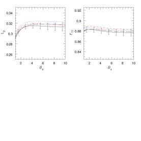
Next, we present in the left panel of Fig.7 the ratio $t_{2}$ of both variances $\langle\gamma_{i{\rm s}}^{2}\rangle$ associated with the two redshift subsamples. Although the dependence on cosmology is rather weak, it could be extracted from the data. Contrary to the aperture mass, $\Omega_{\rm m}$ and $\sigma_{8}$ affect the ratio $t_{2}$ in the same direction as each variance $\langle\gamma_{i{\rm s}}^{2}\rangle$ but with different powers. Therefore, redshift binning still provides additional constraints on cosmology. Finally, we display in the right panel of Fig.7 the cross-correlation coefficient $r_{11}$. As for $M_{\rm ap}$ it is rather high, which translates a strong correlation between both weak-lensing signals, and it only shows a very weak dependence on cosmology. However, since error bars are quite small it might be possible to use $r_{11}$ to further constrain cosmological parameters. On the other hand, this also means that it does not provide a very robust tool to estimate the noise of the survey, unless the cosmological parameters and the source redshifts are known up to a high accuracy.

Fourth-order cumulants

Figure 8: The kurtosis of smoothed shear components $S_{4}$ is plotted for two redshift bins as a function of smoothing angle $\theta_{s}$ (low-$z$ subsample: left panel, high-$z$ subsample: right panel).

Figure 9: The left panel shows $t_{4}$ as a function of smoothing angle $\theta_{s}$. The middle and right panels correspond to $r_{31},r_{13}$ and $r_{22}$ respectively. These quantities are related to the kurtosis of the shear field and are dominated by the noise. We have reduced the error bars by a factor of four for plotting.

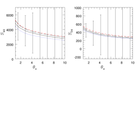
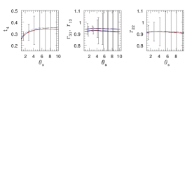
As for $M_{\rm ap}$, we now study the lowest-order cumulants which probe the deviations from Gaussianity. Since the shear components are even random variables we need to go up to fourth order. Since the noise increases very fast with the order this means that non-Gaussianities are more difficult to detect from the shear components than from $M_{\rm ap}$ (where third-order cumulants do not vanish). Thus, we display in Fig.8 the kurtosis $S_{4}$ of the smoothed shear components for both redshift subsamples. As for the skewness of $M_{\rm ap}$, the kurtosis increases for lower source redshifts, and we obtain $S_{40}>S_{04}$. As expected, we can check that the error bars are much larger than for the skewness of $M_{\rm ap}$. In particular, at large angular scales (beyond $6^{\prime}$) it will be difficult to obtain a clear detection of non-Gaussianity. At lower angular scales one should be able to obtain a meaningful measure of $S_{4}$. On the other hand, one should note that the theoretical error bars for $S_{4}$ are actually rather large in this transition regime towards non-linear gravitational structures, so that one cannot expect to obtain strong constraints on cosmology from $S_{4}$. Rather, it is probably safer to use $S_{4}$ to check the broad consistency of the gravitational clustering process.

Next, we show in the left panel of Fig.9 the ratio $t_{4}$ between the fourth-order cumulants associated with both redshift subsamples. As for $M_{\rm ap}$, we get $t_{4}<1$ and the dependence on cosmology is very small. Again, this means that redshift binning does not provide much additional information for fourth-order statistics. On the other hand, a measure of $t_{4}$ could provide a convenient estimate of the noise of the survey with regard to these fourth-order cumulants.

Finally, we present in the middle and right panels of Fig.9 the cross-correlation coefficients $r_{31},r_{13}$ and $r_{22}$. We obtain $r_{31}>r_{13}>r_{22}$. Again, the cross-correlation is large and the dependence on cosmology is very weak and much smaller than error bars. Therefore, these cross-correlations are mostly useful to estimate the noise of the survey rather than the cosmological parameters. We must note that at large angular scales the formula (29) for $\sigma^{2}({\cal R}_{pq})$ yields a negative number (in which case with plot $\sigma=|\sigma^{2}|^{1/2}$. This translates the fact that error bars are so large that errors cannot be linearized in the expression (26) of ${\cal R}_{pq}$. However, in these cases we have $\sigma\ga 1$ so that an accurate estimate of the scatter is not needed: the signal is completely dominated by the noise and useless for practical purposes.

5 Discussion and Future Prospects

In order to derive precise results from weak lensing surveys one must take into account various sources of noise like the intrinsic ellipticity distribution of galaxies and the cosmic variance. Extending a previous study (Valageas, Munshi & Barber 2004) we have introduced these realistic sources of noise in various estimates of cross-correlation statistics between several redshift subsamples. Such studies should help discriminating weak lensing effects from noise and measuring cosmological parameters.

Thus, extending an earlier work (Valageas, Munshi & Barber 2004) where we focused on one-point statistics, we have taken advantage of the high projected density of galaxies $n_{g}$ in the future SNAP survey to divide the source population into two redshift bins. Then, we have computed cross-correlations between these subsamples. Note that our formalism is kept completely general and can be applied to different surveys with or without any overlap in source redshift. We have used two statistics, the aperture mass $M_{\rm ap}$ and the shear components $\gamma_{i{\rm s}}$, to quantify the correlations among redshift bins as a function of the smoothing angle $\theta_{s}$. The underlying model that we have used for computing the cumulant correlators is the same as that of Valageas, Munshi & Barber (2004). This has been tested against numerical simulations for a wide range of smoothing angles and source redshifts and was found to provide good results.

We have considered both second-order cumulants (cross-correlation $r_{11}$) and the lowest-order cumulants which can measure deviations from Gaussianity (third or fourth order for $M_{\rm ap}$ or $\gamma_{i{\rm s}}$). High order cumulants can remove the well-known degeneracy between $\Omega_{\rm m}$ and $\sigma_{8}$ but the relative importance of the noise increases rapidly with order. This makes the aperture mass a better tool than the shear components which require fourth-order statistics. However, note that weak lensing statistics are also sensitive to source redshifts which might prove a significant limitation for any weak lensing survey. We noticed that for a survey such as SNAP one could still obtain interesting information from the shear components after dividing the sample into two redshift bins, while for the aperture mass one could go up to three subsamples. Increasing further the number of subsamples increases the noise of third-order or higher order cumulants and is mostly useless (except for the variance where the error bars are small). We have found that cross-correlations between subsamples do not bring additional information with regard to the constraints on cosmology to those already provided by one-point statistics (except marginally for the second-order moments of the shear). Indeed, different source populations selected by their redshift (in the zero angular separation case) still probe the same density fluctuations at low $z$ (where they are largest). This implies a high value for the various cross-correlation coefficients which are almost independent of cosmological parameters. These properties hold even better for higher orders statistics. However, this feature can be used to estimate the noise of the survey. Therefore, one-point and two-point statistics provide complementary tools: the former can constrain cosmology and check the gravitational clustering process, while the latter can yield an estimate of the noise of the survey.

Recent studies have underlined the importance of joint estimation of cosmological parameters such as galaxy-shear cross correlation, shear-shear correlations along with galaxy-galaxy angular correlations. Deep multi-colour galaxy surveys with photometric redshifts will provide an unique opportunity to study such large numbers of two-point correlation observables to pin-point the background dynamics of the universe as well as non-Gaussianity and bias associated with cosmological density distribution of underlying mass as well as galaxy populations. The statistical machinery developed here will be extremely useful in this direction.

Although the cross correlations and the error terms are defined in this work with a specific filter in mind and we only concentrate on two different statistics the framework developed here has been kept completely general and the formalism can be used to compute the signal to noise related to quantities such as foreground-background galaxy populations (Moessner & Jain 1998). Fluctuations in size distribution of source galaxies can also be used to study the weak lensing convergence directly without having to go through the map making procedure, from shear maps to convergence maps (see e.g. Jain, 2002). Higher order cross-correlation statistics or cumulant correlators we develop here can be useful in probing correlations of such measures of weak lensing convergence with cosmic shear measurements using shapes of background galaxies as observations improve and surveys start to cover a larger part of the sky and probe deeper. Not only these statistics can provide valuable consistency checks among various measures from different surveys, they will also be a useful supplement in constraining cosmological parameters when used along with their one-point counterparts.

Recently Dalal et al. (2002) have investigated the correlation between the smoothed convergence and the value along the line of sight to individual supernovae. However these calculations were done by ignoring non-Gaussian corrections. The formalism developed here takes into account all non-linear corrections from higher order contributions. In our formalism we have shown that such calculations can be treated as a special case of the generic expression derived here in a more general context. These results can not only be used to analyze cross-correlations among various redshift surveys but also to probe supernova weak-lensing cross-correlation. A more detailed analysis will be presented elsewhere.

Although current studies of weak lensing effects have focused on the distortion of background galaxy ellipticities, it has been pointed out recently that such studies can be augmented in the near future by lensing studies of unresolved sources and also of the spatial fluctuations of their integrated diffuse emission. In particular one could study the diffuse background generated at far-infrared wavelengths by dusty star bursts, first stars and galaxies in near-infrared and also the 21cm emission from neutral gas which forms the intergalactic medium prior to reionization. These studies promise to smoothly interpolate from the weak-lensing studies of the cosmic microwave background at very high redshift downto weak lensing studies using galaxy shapes at low redshifts. Cross-correlation studies of one type of surveys with another hold the prospect of mapping the dark matter distribution of the universe at medium redshift. We plan to present results of such analysis in a separate paper.

In almost all weak lensing studies one uses the Born-approximation. Its validity is checked in numerous numerical studies of weak lensing at small angular scales. In addition we have ignored contributions from source clustering and lens coupling. Some of these issues have been studied in Bernardeau (1997), Bernardeau et al (1997) and Schneider et al. (1998). It was found that at large smoothing angular scales these contributions are negligible. In the highly nonlinear regime an accurate picture of galaxy bias is required to deal with these issues but it is still lacking at the moment.

The correlations of galaxy intrinsic ellipticities might yield additional complexities in dealing with shear correlations and elaborate schemes have been developed (Heymans & Heavens 2003, Crittenden et al. 2002). However the extent to which such correlations will affect weak lensing surveys remains somewhat uncertain. It is generally believed that such effects will play a less important role as we increase the survey depth and we can reduce their role through acquisition of photometric redshift (Heymans & Heavens 2003).

It is almost always assumed in all weak lensing studies that the galaxy intrinsic ellipticity distribution is Gaussian although it might not be the case. Any signature of such non-Gaussianity if found by observational teams will have to be included into our analytical calculations. However this can be performed in a straightforward way in our formalism. Clearly, if such intrinsic non-Gaussianities are too large they might even dominate the signal and complicate inferring the observational data.

It became clear that future weak lensing surveys will mostly be limited by sky coverage which determines the scatter due to the finite size of the catalog. The intrinsic ellipticities will only dominate at small angular scales and will not preclude a meaningful estimation even with small sky coverage. In our analysis we have used the plane parallel approximation to compute the higher order non-Gaussianities. However as the survey size increases in the future it will be important to translate these studies using all-sky calculations. A detailed analysis will be presented elsewhere.

Appendix A Scatter of low-order estimators $M_{pq}$ and $H_{pq}$

We give in this appendix the expression of the scatter $\sigma^{2}$ of the various estimators $M_{pq}$ and $H_{pq}$ introduced in section 3 which we need to derive the numerical results presented in section 4. Note that although in our numerical calculations we take the smoothing windows $\theta_{s}$ of different surveys or subsamples to be the same when we compute cross-correlations, this needs not to be the case for the following equations to be valid.

A.1 Aperture Mass

We first consider the aperture mass statistics, where we restrict ourselves to cumulants of order two and three. The dispersions $\sigma^{2}$ of first and second-order estimators are (with $\langle M_{1}\rangle=0$):

$$\sigma^{2}(M_{1})=\langle M_{\rm ap}^{2}\rangle_{c}\left[1+{1\over\rho}\right],\hskip 25.6073pt\sigma^{2}(M_{2})=\langle M_{\rm ap}^{4}\rangle_{c}+\langle M_{\rm ap}^{2}\rangle_{c}^{2}2\left[1+{1\over\rho}\right]^{2},$$ (34)

and:

$$\sigma^{2}(M_{11})=\langle M_{\rm ap1}^{2}M_{\rm ap2}^{2}\rangle_{c}+\langle M_{\rm ap1}M_{\rm ap2}\rangle_{c}^{2}+\langle M_{\rm ap1}^{2}\rangle_{c}\langle M_{\rm ap2}^{2}\rangle_{c}\left[1+{1\over\rho_{1}}\right]\left[1+{1\over\rho_{2}}\right].$$ (35)

Note that in the case $\rho_{1}=\rho_{2}$ the cross-correlation error $\sigma^{2}(M_{11})$ does not become identical to the error $\sigma^{2}(M_{2})$ associated with one survey for the estimator $M_{2}$. This simply reflects our assumption that the intrinsic ellipticities of different galaxies are not correlated and that different surveys or subsamples do not share any galaxy. Of course, it is also possible to handle the case where a certain fraction of the source population is shared by both surveys but we shall not consider this case here. As seen in eqs.(29), (30), we also need the dispersions of cross-products:

$$\sigma^{2}(M_{11};M_{20})=\langle M_{\rm ap1}^{3}M_{\rm ap2}\rangle_{c}+\langle M_{\rm ap1}^{2}\rangle_{c}\langle M_{\rm ap1}M_{\rm ap2}\rangle_{c}2\left[1+{1\over\rho_{1}}\right],\hskip 22.76228pt\sigma^{2}(M_{20};M_{02})=\langle M_{\rm ap1}^{2}M_{\rm ap2}^{2}\rangle_{c}+2\langle M_{\rm ap1}M_{\rm ap2}\rangle_{c}^{2}.$$ (36)

Note that the galaxy intrinsic ellipticities do not contribute to the dispersion of the product $(M_{20}M_{02})$ because we assumed that the two subsamples have no common galaxies. Next, the scatters of third-order estimators are:

$$\sigma^{2}(M_{3})=\langle M_{\rm ap}^{6}\rangle_{c}+\langle M_{\rm ap}^{4}\rangle_{c}\langle M_{\rm ap}^{2}\rangle_{c}\left[15+{9\over\rho}\right]+9\langle M_{\rm ap}^{3}\rangle_{c}^{2}+\langle M_{\rm ap}^{2}\rangle^{3}\left[15+{27\over\rho}+{18\over\rho^{2}}+{6\over\rho^{3}}\right],$$ (37)

and:

$$\sigma^{2}(M_{21}) = \langle M_{\rm ap1}^{4}M_{\rm ap2}^{2}\rangle_{c}+\langle M_{\rm ap1}^{4}\rangle_{c}\langle M_{\rm ap2}^{2}\rangle_{c}\left[1+{1\over\rho_{2}}\right]+8\langle M_{\rm ap1}^{3}M_{\rm ap2}\rangle_{c}\langle M_{\rm ap1}M_{\rm ap2}\rangle_{c}+\langle M_{\rm ap1}^{2}M_{\rm ap2}^{2}\rangle_{c}\langle M_{\rm ap1}^{2}\rangle_{c}\left[6+{4\over\rho_{1}}\right]$$ (38)

$$+4\langle M_{\rm ap1}^{3}\rangle_{c}\langle M_{\rm ap1}M_{\rm ap2}^{2}\rangle_{c}+5\langle M_{\rm ap1}^{2}M_{\rm ap2}\rangle_{c}^{2}+\langle M_{\rm ap1}^{2}\rangle_{c}^{2}\langle M_{\rm ap2}^{2}\rangle_{c}\left[3+{4\over\rho_{1}}+{3\over\rho_{2}}+{2\over\rho_{1}^{2}}+{4\over\rho_{1}\rho_{2}}+{2\over\rho_{1}^{2}\rho_{2}}\right]$$

$$+\langle M_{\rm ap1}M_{\rm ap2}\rangle_{c}^{2}\langle M_{\rm ap1}^{2}\rangle_{c}\left[12+{8\over\rho_{1}}\right].$$

For cross-products we obtain:

$$\sigma^{2}(M_{21};M_{30}) = \langle M_{\rm ap1}^{5}M_{\rm ap2}\rangle_{c}+5\langle M_{\rm ap1}^{4}\rangle_{c}\langle M_{\rm ap1}M_{\rm ap2}\rangle_{c}+\langle M_{\rm ap1}^{3}M_{\rm ap2}\rangle_{c}\langle M_{\rm ap1}^{2}\rangle_{c}\left[10+{6\over\rho_{1}}\right]+9\langle M_{\rm ap1}^{2}M_{\rm ap2}\rangle_{c}\langle M_{\rm ap1}^{3}\rangle_{c}$$ (39)

$$+\langle M_{\rm ap1}M_{\rm ap2}\rangle_{c}\langle M_{\rm ap1}^{2}\rangle_{c}^{2}\left[15+{18\over\rho_{1}}+{6\over\rho_{1}^{2}}\right],$$

$$\sigma^{2}(M_{21};M_{03})=\langle M_{\rm ap1}^{2}M_{\rm ap2}^{4}\rangle_{c}+\langle M_{\rm ap2}^{4}\rangle_{c}\langle M_{\rm ap1}^{2}\rangle_{c}+8\langle M_{\rm ap1}M_{\rm ap2}^{3}\rangle_{c}\langle M_{\rm ap1}M_{\rm ap2}\rangle_{c}+\langle M_{\rm ap1}^{2}M_{\rm ap2}^{2}\rangle_{c}\langle M_{\rm ap2}^{2}\rangle_{c}\left[6+{3\over\rho_{2}}\right]$$ (40)

$$+3\langle M_{\rm ap1}^{2}M_{\rm ap2}\rangle_{c}\langle M_{\rm ap2}^{3}\rangle_{c}+6\langle M_{\rm ap1}M_{\rm ap2}^{2}\rangle_{c}^{2}+\langle M_{\rm ap1}^{2}\rangle_{c}\langle M_{\rm ap2}^{2}\rangle_{c}^{2}\left[3+{3\over\rho_{2}}\right]+\langle M_{\rm ap1}M_{\rm ap2}\rangle_{c}^{2}\langle M_{\rm ap2}^{2}\rangle_{c}\left[12+{6\over\rho_{2}}\right],$$

and:

$$\sigma^{2}(M_{30};M_{03}) = \langle M_{\rm ap1}^{3}M_{\rm ap2}^{3}\rangle_{c}+3\langle M_{\rm ap1}^{3}M_{\rm ap2}\rangle_{c}\langle M_{\rm ap2}^{2}\rangle_{c}+3\langle M_{\rm ap1}M_{\rm ap2}^{3}\rangle_{c}\langle M_{\rm ap1}^{2}\rangle_{c}+9\langle M_{\rm ap1}^{2}M_{\rm ap2}^{2}\rangle_{c}\langle M_{\rm ap1}M_{\rm ap2}\rangle_{c}$$ (41)

$$+9\langle M_{\rm ap1}^{2}M_{\rm ap2}\rangle_{c}\langle M_{\rm ap1}M_{\rm ap2}^{2}\rangle_{c}+9\langle M_{\rm ap1}^{2}\rangle_{c}\langle M_{\rm ap2}^{2}\rangle_{c}\langle M_{\rm ap1}M_{\rm ap2}\rangle_{c}+6\langle M_{\rm ap1}M_{\rm ap2}\rangle_{c}^{3}.$$

As recalled in section 3, following Valageas et al. (2004), it is better to use the cumulant estimators $H_{pq}$ rather than the moment estimators $M_{pq}$, as they show a smaller scatter. Their dispersion can be expressed in terms of the scatter of the estimators $M_{pq}$ as:

$$\sigma^{2}(H_{3})=\sigma^{2}(M_{3})-6\langle M_{\rm ap}^{4}\rangle_{c}\langle M_{\rm ap}^{2}\rangle_{c}-9\langle M_{\rm ap}^{2}\rangle_{c}^{3}\left[1+{1\over\rho}\right],$$ (42)

$$\sigma^{2}(H_{21}) = \sigma^{2}(M_{21})-4\langle M_{\rm ap1}^{3}M_{\rm ap2}\rangle_{c}\langle M_{\rm ap1}M_{\rm ap2}\rangle_{c}-2\langle M_{\rm ap1}^{2}M_{\rm ap2}^{2}\rangle_{c}\langle M_{\rm ap1}^{2}\rangle_{c}-\langle M_{\rm ap1}^{2}\rangle_{c}^{2}\langle M_{\rm ap2}^{2}\rangle_{c}\left[1+{1\over\rho_{2}}\right]$$ (43)

$$-\langle M_{\rm ap1}M_{\rm ap2}\rangle_{c}^{2}\langle M_{\rm ap1}^{2}\rangle_{c}\left[8+{4\over\rho_{1}}\right],$$

$$\sigma^{2}(H_{21};H_{30})=\sigma^{2}(M_{21};M_{30})-2\langle M_{\rm ap1}^{4}\rangle_{c}\langle M_{\rm ap1}M_{\rm ap2}\rangle_{c}-4\langle M_{\rm ap1}^{3}M_{\rm ap2}\rangle_{c}\langle M_{\rm ap1}^{2}\rangle_{c}-\langle M_{\rm ap1}M_{\rm ap2}\rangle_{c}\langle M_{\rm ap1}^{2}\rangle_{c}^{2}\left[9+{6\over\rho_{1}}\right],$$ (44)

$$\sigma^{2}(H_{21};H_{03}) = \sigma^{2}(M_{21};M_{03})-\langle M_{\rm ap2}^{4}\rangle_{c}\langle M_{\rm ap1}^{2}\rangle_{c}-2\langle M_{\rm ap1}M_{\rm ap2}^{3}\rangle_{c}\langle M_{\rm ap1}M_{\rm ap2}\rangle_{c}-3\langle M_{\rm ap1}^{2}M_{\rm ap2}^{2}\rangle_{c}\langle M_{\rm ap2}^{2}\rangle_{c}$$ (45)

$$-\langle M_{\rm ap1}^{2}\rangle_{c}\langle M_{\rm ap2}^{2}\rangle_{c}^{2}\left[3+{3\over\rho_{2}}\right]-6\langle M_{\rm ap1}M_{\rm ap2}\rangle_{c}^{2}\langle M_{\rm ap2}^{2}\rangle_{c},$$

and:

$$\sigma^{2}(H_{30};H_{03})=\sigma^{2}(M_{30};M_{03})-3\langle M_{\rm ap1}^{3}M_{\rm ap2}\rangle_{c}\langle M_{\rm ap2}^{2}\rangle_{c}-3\langle M_{\rm ap1}M_{\rm ap2}^{3}\rangle_{c}\langle M_{\rm ap1}^{2}\rangle_{c}-9\langle M_{\rm ap1}^{2}\rangle_{c}\langle M_{\rm ap2}^{2}\rangle_{c}\langle M_{\rm ap1}M_{\rm ap2}\rangle_{c}.$$ (46)

We can check in eqs.(42)-(46) that the scatter of the estimators $H_{pq}$ is smaller than the dispersion of the estimators $M_{pq}$. Besides, one can note that the galaxy intrinsic ellipticity dispersion only enters the expressions of the scatter of the estimators $H_{pq}$ through the combination $(1+1/\rho)$.

A.2 Shear components

The dispersions of second-order cumulants are given by the same expressions (34)-(36) as the one obtained for the aperture mass. On the other hand, since all odd-order moments of shear components vanish we need to go up to fourth-order moments in order to obtain the first measure of deviations from Gaussianity. Thus, we obtain for fourth-order statistics:

$$\sigma^{2}(M_{4}) = \langle\gamma_{i{\rm s}}^{8}\rangle_{c}+\langle\gamma_{i{\rm s}}^{6}\rangle_{c}\langle\gamma_{i{\rm s}}^{2}\rangle_{c}\left[28+\frac{16}{\rho}\right]+34\langle\gamma_{i{\rm s}}^{4}\rangle_{c}^{2}+\langle\gamma_{i{\rm s}}^{4}\rangle_{c}\langle\gamma_{i{\rm s}}^{2}\rangle_{c}^{2}\left[204+\frac{240}{\rho}+\frac{72}{\rho^{2}}\right]$$ (47)

$$+\langle\gamma_{i{\rm s}}^{2}\rangle_{c}^{4}\left[96+\frac{240}{\rho}+\frac{216}{\rho^{2}}+\frac{96}{\rho^{3}}+\frac{24}{\rho^{4}}\right],$$

$$\sigma^{2}(M_{31}) = \langle\gamma_{i{\rm s}1}^{6}\gamma_{i{\rm s}2}^{2}\rangle_{c}+\langle\gamma_{i{\rm s}1}^{6}\rangle_{c}\langle\gamma_{i{\rm s}2}^{2}\rangle_{c}\left[1+{1\over\rho_{2}}\right]+12\langle\gamma_{i{\rm s}1}^{5}\gamma_{i{\rm s}2}\rangle_{c}\langle\gamma_{i{\rm s}1}\gamma_{i{\rm s}2}\rangle_{c}+\langle\gamma_{i{\rm s}1}^{4}\gamma_{i{\rm s}2}^{2}\rangle_{c}\langle\gamma_{i{\rm s}1}^{2}\rangle_{c}\left[15+{9\over\rho_{1}}\right]$$ (48)

$$+15\langle\gamma_{i{\rm s}1}^{4}\rangle_{c}\langle\gamma_{i{\rm s}1}^{2}\gamma_{i{\rm s}2}^{2}\rangle_{c}+19\langle\gamma_{i{\rm s}1}^{3}\gamma_{i{\rm s}2}\rangle_{c}^{2}+\langle\gamma_{i{\rm s}1}^{4}\rangle_{c}\langle\gamma_{i{\rm s}1}^{2}\rangle_{c}\langle\gamma_{i{\rm s}2}^{2}\rangle_{c}\left[15+{9\over\rho_{1}}+{15\over\rho_{2}}+{9\over\rho_{1}\rho_{2}}\right]+30\langle\gamma_{i{\rm s}1}^{4}\rangle_{c}\langle\gamma_{i{\rm s}1}\gamma_{i{\rm s}2}\rangle_{c}^{2}$$

$$+\langle\gamma_{i{\rm s}1}^{3}\gamma_{i{\rm s}2}\rangle_{c}\langle\gamma_{i{\rm s}1}\gamma_{i{\rm s}2}\rangle_{c}\langle\gamma_{i{\rm s}1}^{2}\rangle_{c}\left[114+{72\over\rho_{1}}\right]+\langle\gamma_{i{\rm s}1}^{2}\gamma_{i{\rm s}2}^{2}\rangle_{c}\langle\gamma_{i{\rm s}1}^{2}\rangle_{c}^{2}\left[45+{54\over\rho_{1}}+{18\over\rho_{1}^{2}}\right]$$

$$+\langle\gamma_{i{\rm s}1}^{2}\rangle_{c}^{3}\langle\gamma_{i{\rm s}2}^{2}\rangle_{c}\left[15+{27\over\rho_{1}}+{15\over\rho_{2}}+{18\over\rho_{1}^{2}}+{27\over\rho_{1}\rho_{2}}+{6\over\rho_{1}^{3}}+{18\over\rho_{1}^{2}\rho_{2}}+{6\over\rho_{1}^{3}\rho_{2}}\right]+\langle\gamma_{i{\rm s}1}\gamma_{i{\rm s}2}\rangle_{c}^{2}\langle\gamma_{i{\rm s}1}^{2}\rangle_{c}^{2}\left[81+{108\over\rho_{1}}+{36\over\rho_{1}^{2}}\right],$$

and:

$$\sigma^{2}(M_{22})=\langle\gamma_{i{\rm s}1}^{4}\gamma_{i{\rm s}2}^{4}\rangle_{c}+16\langle\gamma_{i{\rm s}1}^{3}\gamma_{i{\rm s}2}^{3}\rangle_{c}\langle\gamma_{i{\rm s}1}\gamma_{i{\rm s}2}\rangle_{c}+\langle\gamma_{i{\rm s}1}^{2}\gamma_{i{\rm s}2}^{4}\rangle_{c}\langle\gamma_{i{\rm s}1}^{2}\rangle_{c}\left[6+{4\over\rho_{1}}\right]+\langle\gamma_{i{\rm s}1}^{4}\gamma_{i{\rm s}2}^{2}\rangle_{c}\langle\gamma_{i{\rm s}2}^{2}\rangle_{c}\left[6+{4\over\rho_{2}}\right]+\langle\gamma_{i{\rm s}1}^{4}\rangle_{c}\langle\gamma_{i{\rm s}2}^{4}\rangle_{c}$$ (49)

$$+16\langle\gamma_{i{\rm s}1}\gamma_{i{\rm s}2}^{3}\rangle_{c}\langle\gamma_{i{\rm s}2}\gamma_{i{\rm s}1}^{3}\rangle_{c}+17\langle\gamma_{i{\rm s}1}^{2}\gamma_{i{\rm s}2}^{2}\rangle_{c}^{2}+68\langle\gamma_{i{\rm s}1}^{2}\gamma_{i{\rm s}2}^{2}\rangle_{c}\langle\gamma_{i{\rm s}1}\gamma_{i{\rm s}2}\rangle_{c}^{2}+\langle\gamma_{i{\rm s}1}^{4}\rangle_{c}\langle\gamma_{i{\rm s}2}^{2}\rangle_{c}^{2}\left[3+{4\over\rho_{2}}+{2\over\rho_{2}^{2}}\right]$$

$$+\langle\gamma_{i{\rm s}2}^{4}\rangle_{c}\langle\gamma_{i{\rm s}1}^{2}\rangle_{c}^{2}\left[3+{4\over\rho_{1}}+{2\over\rho_{1}^{2}}\right]+\langle\gamma_{i{\rm s}1}^{3}\gamma_{i{\rm s}2}\rangle_{c}\langle\gamma_{i{\rm s}1}\gamma_{i{\rm s}2}\rangle_{c}\langle\gamma_{i{\rm s}2}^{2}\rangle_{c}\left[48+{32\over\rho_{2}}\right]+\langle\gamma_{i{\rm s}1}\gamma_{i{\rm s}2}^{3}\rangle_{c}\langle\gamma_{i{\rm s}1}\gamma_{i{\rm s}2}\rangle_{c}\langle\gamma_{i{\rm s}1}^{2}\rangle_{c}\left[48+{32\over\rho_{1}}\right]$$

$$+\langle\gamma_{i{\rm s}1}^{2}\gamma_{i{\rm s}2}^{2}\rangle_{c}\langle\gamma_{i{\rm s}1}^{2}\rangle_{c}\langle\gamma_{i{\rm s}2}^{2}\rangle_{c}\left[34+{24\over\rho_{1}}+{24\over\rho_{2}}+{16\over\rho_{1}\rho_{2}}\right]+20\langle\gamma_{i{\rm s}1}\gamma_{i{\rm s}2}\rangle_{c}^{4}+\langle\gamma_{i{\rm s}1}^{2}\rangle_{c}\langle\gamma_{i{\rm s}2}^{2}\rangle_{c}\langle\gamma_{i{\rm s}1}\gamma_{i{\rm s}2}\rangle_{c}^{2}\left[68+{48\over\rho_{1}}+{48\over\rho_{2}}+{32\over\rho_{1}\rho_{2}}\right]$$

$$+\langle\gamma_{i{\rm s}1}^{2}\rangle_{c}^{2}\langle\gamma_{i{\rm s}2}^{2}\rangle_{c}^{2}\left[8+{12\over\rho_{2}}+{12\over\rho_{1}}+{6\over\rho_{1}^{2}}+{6\over\rho_{2}^{2}}+{16\over\rho_{1}\rho_{2}}+{8\over\rho_{1}^{2}\rho_{2}}+{8\over\rho_{2}^{2}\rho_{1}}+{4\over\rho_{1}^{2}\rho_{2}^{2}}\right].$$

Next, for cross-products we obtain:

$$\sigma^{2}(M_{31};M_{40}) = \langle\gamma_{i{\rm s}1}^{7}\gamma_{i{\rm s}2}\rangle_{c}+7\langle\gamma_{i{\rm s}1}^{6}\rangle_{c}\langle\gamma_{i{\rm s}1}\gamma_{i{\rm s}2}\rangle_{c}+\langle\gamma_{i{\rm s}1}^{5}\gamma_{i{\rm s}2}\rangle_{c}\langle\gamma_{i{\rm s}1}^{2}\rangle_{c}\left[21+{12\over\rho_{1}}\right]+34\langle\gamma_{i{\rm s}1}^{3}\gamma_{i{\rm s}2}\rangle_{c}\langle\gamma_{i{\rm s}1}^{4}\rangle_{c}$$ (50)

$$+\langle\gamma_{i{\rm s}1}^{3}\gamma_{i{\rm s}2}\rangle_{c}\langle\gamma_{i{\rm s}1}^{2}\rangle_{c}^{2}\left[102+{120\over\rho_{1}}+{36\over\rho_{1}^{2}}\right]+\langle\gamma_{i{\rm s}1}^{4}\rangle_{c}\langle\gamma_{i{\rm s}1}\gamma_{i{\rm s}2}\rangle_{c}\langle\gamma_{i{\rm s}1}^{2}\rangle_{c}\left[102+{60\over\rho_{1}}\right]$$

$$+\langle\gamma_{i{\rm s}1}\gamma_{i{\rm s}2}\rangle_{c}\langle\gamma_{i{\rm s}1}^{2}\rangle_{c}^{3}\left[96+{180\over\rho_{1}}+{108\over\rho_{1}^{2}}+{24\over\rho_{1}^{3}}\right],$$

$$\sigma^{2}(M_{31};M_{04})=\langle\gamma_{i{\rm s}1}^{3}\gamma_{i{\rm s}2}^{5}\rangle_{c}+3\langle\gamma_{i{\rm s}1}\gamma_{i{\rm s}2}^{5}\rangle_{c}\langle\gamma_{i{\rm s}1}^{2}\rangle_{c}+\langle\gamma_{i{\rm s}1}^{3}\gamma_{i{\rm s}2}^{3}\rangle_{c}\langle\gamma_{i{\rm s}2}^{2}\rangle_{c}\left[10+{4\over\rho_{2}}\right]+15\langle\gamma_{i{\rm s}1}^{2}\gamma_{i{\rm s}2}^{4}\rangle_{c}\langle\gamma_{i{\rm s}1}\gamma_{i{\rm s}2}\rangle_{c}$$ (51)

$$+4\langle\gamma_{i{\rm s}1}^{3}\gamma_{i{\rm s}2}\rangle_{c}\langle\gamma_{i{\rm s}2}^{4}\rangle_{c}+30\langle\gamma_{i{\rm s}1}^{2}\gamma_{i{\rm s}2}^{2}\rangle_{c}\langle\gamma_{i{\rm s}1}\gamma_{i{\rm s}2}^{3}\rangle_{c}+\langle\gamma_{i{\rm s}1}^{3}\gamma_{i{\rm s}2}\rangle_{c}\langle\gamma_{i{\rm s}2}^{2}\rangle_{c}^{2}\left[12+{12\over\rho_{2}}\right]$$

$$+12\langle\gamma_{i{\rm s}2}^{4}\rangle_{c}\langle\gamma_{i{\rm s}1}\gamma_{i{\rm s}2}\rangle_{c}\langle\gamma_{i{\rm s}1}^{2}\rangle_{c}+\langle\gamma_{i{\rm s}1}\gamma_{i{\rm s}2}^{3}\rangle_{c}\langle\gamma_{i{\rm s}1}^{2}\rangle_{c}\langle\gamma_{i{\rm s}2}^{2}\rangle_{c}\left[30+{12\over\rho_{2}}\right]+60\langle\gamma_{i{\rm s}1}\gamma_{i{\rm s}2}^{3}\rangle_{c}\langle\gamma_{i{\rm s}1}\gamma_{i{\rm s}2}\rangle_{c}^{2}$$

$$+\langle\gamma_{i{\rm s}1}^{2}\gamma_{i{\rm s}2}^{2}\rangle_{c}\langle\gamma_{i{\rm s}1}\gamma_{i{\rm s}2}\rangle_{c}\langle\gamma_{i{\rm s}2}^{2}\rangle_{c}\left[90+{36\over\rho_{2}}\right]+\langle\gamma_{i{\rm s}1}\gamma_{i{\rm s}2}\rangle_{c}\langle\gamma_{i{\rm s}1}^{2}\rangle_{c}\langle\gamma_{i{\rm s}2}^{2}\rangle_{c}^{2}\left[36+{36\over\rho_{2}}\right]+\langle\gamma_{i{\rm s}1}\gamma_{i{\rm s}2}\rangle_{c}^{3}\langle\gamma_{i{\rm s}2}^{2}\rangle_{c}\left[60+{24\over\rho_{2}}\right],$$

$$\sigma^{2}(M_{40};M_{04}) = \langle\gamma_{i{\rm s}1}^{4}\gamma_{i{\rm s}2}^{4}\rangle_{c}+6\langle\gamma_{i{\rm s}1}^{2}\gamma_{i{\rm s}2}^{4}\rangle_{c}\langle\gamma_{i{\rm s}1}^{2}\rangle_{c}+6\langle\gamma_{i{\rm s}1}^{4}\gamma_{i{\rm s}2}^{2}\rangle_{c}\langle\gamma_{i{\rm s}2}^{2}\rangle_{c}+16\langle\gamma_{i{\rm s}1}^{3}\gamma_{i{\rm s}2}^{3}\rangle_{c}\langle\gamma_{i{\rm s}1}\gamma_{i{\rm s}2}\rangle_{c}+16\langle\gamma_{i{\rm s}1}^{3}\gamma_{i{\rm s}2}\rangle_{c}\langle\gamma_{i{\rm s}1}\gamma_{i{\rm s}2}^{3}\rangle_{c}$$ (52)

$$+18\langle\gamma_{i{\rm s}1}^{2}\gamma_{i{\rm s}2}^{2}\rangle_{c}^{2}+48\langle\gamma_{i{\rm s}1}\gamma_{i{\rm s}2}^{3}\rangle_{c}\langle\gamma_{i{\rm s}1}^{2}\rangle_{c}\langle\gamma_{i{\rm s}1}\gamma_{i{\rm s}2}\rangle_{c}+48\langle\gamma_{i{\rm s}1}^{3}\gamma_{i{\rm s}2}\rangle_{c}\langle\gamma_{i{\rm s}2}^{2}\rangle_{c}\langle\gamma_{i{\rm s}1}\gamma_{i{\rm s}2}\rangle_{c}+36\langle\gamma_{i{\rm s}1}^{2}\gamma_{i{\rm s}2}^{2}\rangle_{c}\langle\gamma_{i{\rm s}1}^{2}\rangle_{c}\langle\gamma_{i{\rm s}2}^{2}\rangle_{c}$$

$$+72\langle\gamma_{i{\rm s}1}^{2}\gamma_{i{\rm s}2}^{2}\rangle_{c}\langle\gamma_{i{\rm s}1}\gamma_{i{\rm s}2}\rangle_{c}^{2}+72\langle\gamma_{i{\rm s}1}\gamma_{i{\rm s}2}\rangle_{c}^{2}\langle\gamma_{i{\rm s}1}^{2}\rangle_{c}\langle\gamma_{i{\rm s}2}^{2}\rangle_{c}+24\langle\gamma_{i{\rm s}1}\gamma_{i{\rm s}2}\rangle_{c}^{4},$$

and:

$$\sigma^{2}(M_{22};M_{40})=\langle\gamma_{i{\rm s}1}^{6}\gamma_{i{\rm s}2}^{2}\rangle_{c}+\langle\gamma_{i{\rm s}1}^{6}\rangle_{c}\langle\gamma_{i{\rm s}2}^{2}\rangle_{c}+12\langle\gamma_{i{\rm s}1}^{5}\gamma_{i{\rm s}2}\rangle_{c}\langle\gamma_{i{\rm s}1}\gamma_{i{\rm s}2}\rangle_{c}+\langle\gamma_{i{\rm s}1}^{4}\gamma_{i{\rm s}2}^{2}\rangle_{c}\langle\gamma_{i{\rm s}1}^{2}\rangle_{c}\left[15+{8\over\rho_{1}}\right]+14\langle\gamma_{i{\rm s}1}^{4}\rangle_{c}\langle\gamma_{i{\rm s}1}^{2}\gamma_{i{\rm s}2}^{2}\rangle_{c}$$ (53)

$$+20\langle\gamma_{i{\rm s}1}^{3}\gamma_{i{\rm s}2}\rangle_{c}^{2}+\langle\gamma_{i{\rm s}1}^{2}\gamma_{i{\rm s}2}^{2}\rangle_{c}\langle\gamma_{i{\rm s}1}^{2}\rangle_{c}^{2}\left[42+{48\over\rho_{1}}+{12\over\rho_{1}^{2}}\right]+\langle\gamma_{i{\rm s}1}^{4}\rangle_{c}\langle\gamma_{i{\rm s}1}^{2}\rangle_{c}\langle\gamma_{i{\rm s}2}^{2}\rangle_{c}\left[14+{8\over\rho_{1}}\right]+28\langle\gamma_{i{\rm s}1}^{4}\rangle_{c}\langle\gamma_{i{\rm s}1}\gamma_{i{\rm s}2}\rangle_{c}^{2}$$

$$+\langle\gamma_{i{\rm s}1}^{3}\gamma_{i{\rm s}2}\rangle_{c}\langle\gamma_{i{\rm s}1}\gamma_{i{\rm s}2}\rangle_{c}\langle\gamma_{i{\rm s}1}^{2}\rangle_{c}\left[120+{64\over\rho_{1}}\right]+\langle\gamma_{i{\rm s}1}^{2}\rangle_{c}^{3}\langle\gamma_{i{\rm s}2}^{2}\rangle_{c}\left[12+{24\over\rho_{1}}+{12\over\rho_{1}^{2}}\right]+\langle\gamma_{i{\rm s}1}\gamma_{i{\rm s}2}\rangle_{c}^{2}\langle\gamma_{i{\rm s}1}^{2}\rangle_{c}^{2}\left[84+{96\over\rho_{1}}+{24\over\rho_{1}^{2}}\right].$$

Finally, we obtain for the estimators $H_{pq}$:

$$\sigma^{2}(H_{4})=\sigma^{2}(M_{4})-12\langle\gamma_{i{\rm s}}^{6}\rangle_{c}\langle\gamma_{i{\rm s}}^{2}\rangle_{c}-12\langle\gamma_{i{\rm s}}^{4}\rangle_{c}\langle\gamma_{i{\rm s}}^{2}\rangle_{c}^{2}\left[11+{8\over\rho}\right]-72\langle\gamma_{i{\rm s}}^{2}\rangle_{c}^{4}\left[1+{1\over\rho}\right]^{2},$$ (54)

$$\sigma^{2}(H_{31}) = \sigma^{2}(M_{31})-6\langle\gamma_{i{\rm s}1}^{5}\gamma_{i{\rm s}2}\rangle_{c}\langle\gamma_{i{\rm s}1}\gamma_{i{\rm s}2}\rangle_{c}-6\langle\gamma_{i{\rm s}1}^{4}\gamma_{i{\rm s}2}^{2}\rangle_{c}\langle\gamma_{i{\rm s}1}^{2}\rangle_{c}-6\langle\gamma_{i{\rm s}1}^{4}\rangle_{c}\langle\gamma_{i{\rm s}1}^{2}\rangle_{c}\langle\gamma_{i{\rm s}2}^{2}\rangle_{c}\left[1+{1\over\rho_{2}}\right]-21\langle\gamma_{i{\rm s}1}^{4}\rangle_{c}\langle\gamma_{i{\rm s}1}\gamma_{i{\rm s}2}\rangle_{c}^{2}$$ (55)

$$-\langle\gamma_{i{\rm s}1}^{3}\gamma_{i{\rm s}2}\rangle_{c}\langle\gamma_{i{\rm s}1}\gamma_{i{\rm s}2}\rangle_{c}\langle\gamma_{i{\rm s}1}^{2}\rangle_{c}\left[78+{36\over\rho_{1}}\right]-\langle\gamma_{i{\rm s}1}^{2}\gamma_{i{\rm s}2}^{2}\rangle_{c}\langle\gamma_{i{\rm s}1}^{2}\rangle_{c}^{2}\left[27+{18\over\rho_{1}}\right]-\langle\gamma_{i{\rm s}1}^{2}\rangle_{c}^{3}\langle\gamma_{i{\rm s}2}^{2}\rangle_{c}9\left[1+{1\over\rho_{1}}\right]\left[1+{1\over\rho_{2}}\right]$$

$$-\langle\gamma_{i{\rm s}1}\gamma_{i{\rm s}2}\rangle_{c}^{2}\langle\gamma_{i{\rm s}1}^{2}\rangle_{c}^{2}\left[79+{104\over\rho_{1}}+{34\over\rho_{1}^{2}}\right],$$

$$\sigma^{2}(H_{22}) = \sigma^{2}(M_{22})-8\langle\gamma_{i{\rm s}1}^{3}\gamma_{i{\rm s}2}^{3}\rangle_{c}\langle\gamma_{i{\rm s}1}\gamma_{i{\rm s}2}\rangle_{c}-2\langle\gamma_{i{\rm s}1}^{2}\gamma_{i{\rm s}2}^{4}\rangle_{c}\langle\gamma_{i{\rm s}1}^{2}\rangle_{c}-2\langle\gamma_{i{\rm s}1}^{4}\gamma_{i{\rm s}2}^{2}\rangle_{c}\langle\gamma_{i{\rm s}2}^{2}\rangle_{c}-48\langle\gamma_{i{\rm s}1}^{2}\gamma_{i{\rm s}2}^{2}\rangle_{c}\langle\gamma_{i{\rm s}1}\gamma_{i{\rm s}2}\rangle_{c}^{2}$$ (56)

$$-\langle\gamma_{i{\rm s}1}^{4}\rangle_{c}\langle\gamma_{i{\rm s}2}^{2}\rangle_{c}^{2}-\langle\gamma_{i{\rm s}2}^{4}\rangle_{c}\langle\gamma_{i{\rm s}1}^{2}\rangle_{c}^{2}-\langle\gamma_{i{\rm s}1}^{3}\gamma_{i{\rm s}2}\rangle_{c}\langle\gamma_{i{\rm s}1}\gamma_{i{\rm s}2}\rangle_{c}\langle\gamma_{i{\rm s}2}^{2}\rangle_{c}\left[32+{16\over\rho_{2}}\right]-\langle\gamma_{i{\rm s}1}\gamma_{i{\rm s}2}^{3}\rangle_{c}\langle\gamma_{i{\rm s}1}\gamma_{i{\rm s}2}\rangle_{c}\langle\gamma_{i{\rm s}1}^{2}\rangle_{c}\left[32+{16\over\rho_{1}}\right]$$

$$-\langle\gamma_{i{\rm s}1}^{2}\gamma_{i{\rm s}2}^{2}\rangle_{c}\langle\gamma_{i{\rm s}1}^{2}\rangle_{c}\langle\gamma_{i{\rm s}2}^{2}\rangle_{c}\left[18+{8\over\rho_{1}}+{8\over\rho_{2}}\right]-16\langle\gamma_{i{\rm s}1}\gamma_{i{\rm s}2}\rangle_{c}^{4}-\langle\gamma_{i{\rm s}1}^{2}\rangle_{c}\langle\gamma_{i{\rm s}2}^{2}\rangle_{c}\langle\gamma_{i{\rm s}1}\gamma_{i{\rm s}2}\rangle_{c}^{2}\left[52+{32\over\rho_{1}}+{32\over\rho_{2}}+{16\over\rho_{1}\rho_{2}}\right]$$

$$-\langle\gamma_{i{\rm s}1}^{2}\rangle_{c}^{2}\langle\gamma_{i{\rm s}2}^{2}\rangle_{c}^{2}\left[4+{4\over\rho_{1}}+{4\over\rho_{2}}+{2\over\rho_{1}^{2}}+{2\over\rho_{2}^{2}}\right],$$

$$\sigma^{2}(H_{31};H_{40}) = \sigma^{2}(M_{31};M_{40})-3\langle\gamma_{i{\rm s}1}^{6}\rangle_{c}\langle\gamma_{i{\rm s}1}\gamma_{i{\rm s}2}\rangle_{c}-9\langle\gamma_{i{\rm s}1}^{5}\gamma_{i{\rm s}2}\rangle_{c}\langle\gamma_{i{\rm s}1}^{2}\rangle_{c}-\langle\gamma_{i{\rm s}1}^{3}\gamma_{i{\rm s}2}\rangle_{c}\langle\gamma_{i{\rm s}1}^{2}\rangle_{c}^{2}\left[66+{48\over\rho_{1}}\right]$$ (57)

$$-\langle\gamma_{i{\rm s}1}^{4}\rangle_{c}\langle\gamma_{i{\rm s}1}\gamma_{i{\rm s}2}\rangle_{c}\langle\gamma_{i{\rm s}1}^{2}\rangle_{c}\left[66+{24\over\rho_{1}}\right]-\langle\gamma_{i{\rm s}1}\gamma_{i{\rm s}2}\rangle_{c}\langle\gamma_{i{\rm s}1}^{2}\rangle_{c}^{3}\left[72+{108\over\rho_{1}}+{36\over\rho_{1}^{2}}\right],$$

$$\sigma^{2}(H_{31};H_{04})=\sigma^{2}(M_{31};M_{04})-3\langle\gamma_{i{\rm s}1}\gamma_{i{\rm s}2}^{5}\rangle_{c}\langle\gamma_{i{\rm s}1}^{2}\rangle_{c}-6\langle\gamma_{i{\rm s}1}^{3}\gamma_{i{\rm s}2}^{3}\rangle_{c}\langle\gamma_{i{\rm s}2}^{2}\rangle_{c}-3\langle\gamma_{i{\rm s}1}^{2}\gamma_{i{\rm s}2}^{4}\rangle_{c}\langle\gamma_{i{\rm s}1}\gamma_{i{\rm s}2}\rangle_{c}-\langle\gamma_{i{\rm s}1}^{3}\gamma_{i{\rm s}2}\rangle_{c}\langle\gamma_{i{\rm s}1}^{2}\rangle_{c}^{2}\left[12+{12\over\rho_{2}}\right]$$ (58)

$$-12\langle\gamma_{i{\rm s}2}^{4}\rangle_{c}\langle\gamma_{i{\rm s}1}\gamma_{i{\rm s}2}\rangle_{c}\langle\gamma_{i{\rm s}1}^{2}\rangle_{c}-\langle\gamma_{i{\rm s}1}\gamma_{i{\rm s}2}^{3}\rangle_{c}\langle\gamma_{i{\rm s}1}^{2}\rangle_{c}\langle\gamma_{i{\rm s}2}^{2}\rangle_{c}\left[30+{12\over\rho_{2}}\right]-24\langle\gamma_{i{\rm s}1}\gamma_{i{\rm s}2}^{3}\rangle_{c}\langle\gamma_{i{\rm s}1}\gamma_{i{\rm s}2}\rangle_{c}^{2}$$

$$-54\langle\gamma_{i{\rm s}1}^{2}\gamma_{i{\rm s}2}^{2}\rangle_{c}\langle\gamma_{i{\rm s}1}\gamma_{i{\rm s}2}\rangle_{c}\langle\gamma_{i{\rm s}2}^{2}\rangle_{c}-\langle\gamma_{i{\rm s}1}\gamma_{i{\rm s}2}\rangle_{c}\langle\gamma_{i{\rm s}1}^{2}\rangle_{c}\langle\gamma_{i{\rm s}2}^{2}\rangle_{c}^{2}\left[36+{36\over\rho_{2}}\right]-36\langle\gamma_{i{\rm s}1}\gamma_{i{\rm s}2}\rangle_{c}^{3}\langle\gamma_{i{\rm s}2}^{2}\rangle_{c},$$

$$\sigma^{2}(H_{40};H_{04}) = \sigma^{2}(M_{40};M_{04})-6\langle\gamma_{i{\rm s}1}^{2}\gamma_{i{\rm s}2}^{4}\rangle_{c}\langle\gamma_{i{\rm s}1}^{2}\rangle_{c}-6\langle\gamma_{i{\rm s}1}^{4}\gamma_{i{\rm s}2}^{2}\rangle_{c}\langle\gamma_{i{\rm s}2}^{2}\rangle_{c}-48\langle\gamma_{i{\rm s}1}\gamma_{i{\rm s}2}^{3}\rangle_{c}\langle\gamma_{i{\rm s}1}^{2}\rangle_{c}\langle\gamma_{i{\rm s}1}\gamma_{i{\rm s}2}\rangle_{c}$$ (59)

$$-48\langle\gamma_{i{\rm s}1}^{3}\gamma_{i{\rm s}2}\rangle_{c}\langle\gamma_{i{\rm s}2}^{2}\rangle_{c}\langle\gamma_{i{\rm s}1}\gamma_{i{\rm s}2}\rangle_{c}-36\langle\gamma_{i{\rm s}1}^{2}\gamma_{i{\rm s}2}^{2}\rangle_{c}\langle\gamma_{i{\rm s}1}^{2}\rangle_{c}\langle\gamma_{i{\rm s}2}^{2}\rangle_{c}-72\langle\gamma_{i{\rm s}1}\gamma_{i{\rm s}2}\rangle_{c}^{2}\langle\gamma_{i{\rm s}1}^{2}\rangle_{c}\langle\gamma_{i{\rm s}2}^{2}\rangle_{c},$$

$$\sigma^{2}(H_{22};H_{40}) = \sigma^{2}(M_{22};M_{40})-\langle\gamma_{i{\rm s}1}^{6}\rangle_{c}\langle\gamma_{i{\rm s}2}^{2}\rangle_{c}-4\langle\gamma_{i{\rm s}1}^{5}\gamma_{i{\rm s}2}\rangle_{c}\langle\gamma_{i{\rm s}1}\gamma_{i{\rm s}2}\rangle_{c}-7\langle\gamma_{i{\rm s}1}^{4}\gamma_{i{\rm s}2}^{2}\rangle_{c}\langle\gamma_{i{\rm s}1}^{2}\rangle_{c}-\langle\gamma_{i{\rm s}1}^{2}\gamma_{i{\rm s}2}^{2}\rangle_{c}\langle\gamma_{i{\rm s}1}^{2}\rangle_{c}^{2}\left[30+{24\over\rho_{1}}\right]$$ (60)

$$-\langle\gamma_{i{\rm s}1}^{4}\rangle_{c}\langle\gamma_{i{\rm s}1}^{2}\rangle_{c}\langle\gamma_{i{\rm s}2}^{2}\rangle_{c}\left[14+{8\over\rho_{1}}\right]-16\langle\gamma_{i{\rm s}1}^{4}\rangle_{c}\langle\gamma_{i{\rm s}1}\gamma_{i{\rm s}2}\rangle_{c}^{2}-\langle\gamma_{i{\rm s}1}^{3}\gamma_{i{\rm s}2}\rangle_{c}\langle\gamma_{i{\rm s}1}\gamma_{i{\rm s}2}\rangle_{c}\langle\gamma_{i{\rm s}1}^{2}\rangle_{c}\left[72+{16\over\rho_{1}}\right]$$

$$-\langle\gamma_{i{\rm s}1}^{2}\rangle_{c}^{3}\langle\gamma_{i{\rm s}2}^{2}\rangle_{c}\left[12+{24\over\rho_{1}}+{12\over\rho_{1}^{2}}\right]-\langle\gamma_{i{\rm s}1}\gamma_{i{\rm s}2}\rangle_{c}^{2}\langle\gamma_{i{\rm s}1}^{2}\rangle_{c}^{2}\left[60+{48\over\rho_{1}}\right].$$

As for the aperture mass, we can check that the scatter of these estimators $H_{pq}$ is smaller than for their counterparts $M_{pq}$ and that the galaxy intrinsic ellipticities only enter their dispersion through the combination $(1+1/\rho)$.

References

- [1] Bacon D.J., Refregier A., Ellis R.S., 2000, MNRAS, 318, 625
- [2] Barber A. J., Munshi D., Valageas P., 2004, MNRAS, 347, 665
- [3] Bernardeau F., Schaeffer R., 1992, A&A, 255, 1
- [4] Bernardeau F., Valageas P., 2000, A&A, 364, 1
- [5] Bernardeau F., Van Waerbeke L., Mellier Y., 1997, A&A, 322, 1
- [6] Couchman H. M. P., Barber A. J., Thomas P. A., 1999, MNRAS, 308, 180
- [7] Crittenden R.G., Natarajan P., Pen U., Theuns T., 2001, ApJ, 559, 552
- [8] Cooray A., Sheth R., Phys.Rept. 372 (2002) 1, 797
- [9] Dalal N., Holz D. E., Chen X., Frieman J. A., (2003), ApJ,585,11
- [10] Fry J.N., 1984, ApJ, 279, 499
- [11] Heymans C., Heavens A., MNRAS, 339 (2003) 711
- [12] Hoekstra H., Yee H. K. C., Gladders M. D., 2002, ApJ, 577, 595
- [13] Jain B., 2002, ApJ, 580, L3
- [14] Jain B., Seljak U., 1997, ApJ, 484, 560
- [15] Jain B., Seljak U., White S.D.M., 2000, ApJ, 530, 547
- [16] Jaroszyn’ski M., Park C., Paczynski B., Gott J.R., 1990, ApJ, 365, 22
- [17] Kaiser N., 1992, ApJ, 388, 272
- [18] Kaiser N., Squires G., Fahlman G., Woods D., 1994, in: Durret F., Mazure A., Tran Thanh Van J. (eds.) Clusters of galaxies. Editions Frontieres
- [19] Kaiser N., 1998, ApJ, 498, 26
- [20] Munshi D., Jain B., 2000, MNRAS, 318, 109
- [21] Munshi D., Jain B., 2001, MNRAS, 322, 107
- [22] Munshi D., 2000, MNRAS, 318, 145
- [23] Munshi D., Melott A.L., Coles P., 1999, MNRAS, 311, 149
- [24] Munshi D., Coles P., 2003, MNRAS, 338, 846
- [25] Munshi D., Valageas P., Barber A. J., 2004, MNRAS
- [26] Peacock J.A., Dodds S.J., 1996, MNRAS, 280, L19
- [27] Peacock J.A., Smith R. E., 2000, MNRAS, 318, 1144
- [28] Refregier A. et al., astro-ph/0304419
- [29] Schaeffer R., 1984, A&A, 134, L15
- [30] Schneider P., 1996, MNRAS, 283, 837
- [31] Schneider P., van Waerbeke L., Jain B., Kruse G., 1998, MNRAS, 296, 873
- [32] Schneider P., Weiss A., 1988, ApJ, 330,1
- [33] Stebbins A., 1996, astro-ph/9609149
- [34] Szapudi I., Szalay A.S., 1993, ApJ, 408, 43
- [35] Szapudi I., Szalay A.S., 1997, ApJ, 481, L1
- [36] Takada & Jain 2002, MNRAS, 344 (2003) 857
- [37] Takada & Jain 2003a, MNRAS, 346 (2003) 949
- [38] Takada & Jain 2003b, MNRAS, 344 (2003) 857
- [39] Valageas P., 2000a, A&A, 354, 767
- [40] Valageas P., 2000b, A&A, 356, 771
- [41] Valageas P., Barber A. J., Munshi D., 2004, MNRAS, 347, 652
- [42] Van Waerbeke L., Bernardeau F., Mellier Y., 1999, A& A, 342, 15
- [43] Van Waerbeke L., Hamana T., Scoccimarro R., Colombi S., Bernardeau F., 2001, MNRAS, 322, 918
- [44] Villumsen J.V., 1996, MNRAS, 281, 369
- [45] Van Waerbeke L., Mellier Y., Pelló R., Pen U.-L., McCracken
Appendix A Scatter of low-order estimators and