Angular Clustering of Galaxies at 3.6 µm from the SWIRE survey

Abstract

We present the first analysis of large-scale clustering from the Spitzer Wide-area InfraRed Extragalactic legacy survey: SWIRE. We compute the angular correlation function of galaxies selected to have 3.6 µm fluxes brighter than 32 $\mu$Jy in three fields totaling two square degrees in area. In each field we detect clustering with a high level of significance. The amplitude and slope of the correlation function is consistent between the three fields and is modeled as $w(\theta)=A\theta^{1-\gamma}$ with $A=(0.6\pm 0.3)\times 10^{-3},\gamma=2.03\pm 0.10$. With a fixed slope of $\gamma=1.8$, we obtain an amplitude of $A=(1.7\pm 0.1)\times 10^{-3}$. Assuming an equivalent depth of $K\approx 18.7$ mag we find our errors are smaller but our results are consistent with existing clustering measurements in $K$-band surveys and with stable clustering models. We estimate our median redshift $z\simeq 0.75$ and this allows us to obtain an estimate of the three-dimensional correlation function $\xi(r)$, for which we find $r_{0}=4.4\pm 0.1h^{-1}$ Mpc.

1 Introduction

The Spitzer Wide-area InfraRed Extragalactic legacy survey, SWIRE (Lonsdale et al., 2003, 2004), has recently begun observations. The survey was designed to dramatically enhance our understanding of galaxy evolution. We will study the history of star-formation, the assembly of stellar mass, the nature and impact of accretion processes in active nuclei, and the influence of environment on these processes at all scales. The survey will detect around two million galaxies at infrared wavelengths ranging from 3.6 µm to 160 µm, over 50 square degrees.

The analysis of the clustering of galaxies has been an important tool in cosmology for many years (e.g., Peebles, 1980). Originally galaxies were assumed to trace the mass density field (modulo some “bias” factor) and their clustering was used to constrain cosmological models. For example, the angular correlation function of the APM galaxy survey was able to rule out the once standard cold dark matter model (Maddox et al., 1990). Today the cosmological models are usually constrained by observations of the cosmic microwave background (e.g. Bennett et al. 2003) and conventional models of the evolution of structure under gravity can then provide us with estimates of the statistical properties of the mass density field. Hence studies of galaxy clustering can now be used to understand the relationship between galaxy formation and the mass field, i.e. the galaxy bias (e.g. Benson et al. 2001).

In this paper we take the first step towards an understanding of the clustering of the SWIRE sources, by measuring the angular correlation function of those galaxies that are detected at 3.6 µm ($L$ band) with the Infrared Array Camera (IRAC). For galaxies at $z\approx 0.6-0.7$ the 3.6 µm band probes the rest-frame $K$-band and so their clustering can be compared directly with that from local $K$-band surveys such as the Two Micron All Sky Survey (2MASS; Maller et al., 2003). At this wavelength, the emission is dominated by older stellar populations so these galaxies are tracing the sites of star-formation in the distant past and we are probing the bias at even earlier epochs.

2 Catalogs and Sample Selection

2.1 Catalogs

The catalogs that we are using are all the ones that were available in March 2004, i.e. our validation “tile” in the Lockman hole region (0.4 deg²) and two tiles in the ELAIS N1 region (each 0.8 deg²). The data are available from the Spitzer Science Archive as programs PROGID=142 and PROGID=185 respectively. The data processing will be described in detail in a future paper (Surace et al., 2004). The 5$\sigma$ limit of the 3.6 $\mu$m catalogs is $S_{3.6}=3.7$ $\mu$Jy (Lonsdale et al., 2004); in the analysis that follows we consider only those galaxies that have $S_{3.6}\geq 32$ $\mu$Jy, a flux-limited sample with typically very high signal-to-noise ratio ($>40$).

2.2 Star/galaxy Separation

Contaminating stars will reduce the galaxy clustering signal, and so we have investigated two procedures for separating stars and galaxies. The first method uses our supporting optical data in the central 0.3 square degrees of the Lockman tile. We select objects with optical counterparts and detections in at least four bands (U, $g^{\prime}$, $r^{\prime}$, $i^{\prime}$, 3.6 µm, 4.5 µm). From these, we reject objects that are morphologically classified as stellar and are brighter than $r^{\prime}<23$ mag (below this limit, the star/galaxy separation becomes unreliable). We also reject those objects which have good optical/infrared data, but for which no galaxy or AGN template spectrum provides a good fit (Rowan-Robinson et al., 2004). This method provided us with 872 stars and 2115 galaxies, with 727 IRAC sources rejected. The stellar number count models of Jarrett et al. (1994) predict 620 sources, therefore we expect the stellar contamination in our catalog to be small.

In the second method we use the IRAC color from 3.6 to 4.5 µm: $C_{12}=\log(S_{3.6}/S_{4.5})$. We model this color above $S_{3.6}>500$ $\mu$Jy as a Gaussian (assuming these to be stars, but fitting only to the positive half of the distribution to avoid residual contamination from galaxies). We find a mean $\bar{C}_{12}=0.235$ and $\sigma_{c_{12}}=0.014$. We then apply a three-sigma cut and reject stars with $0.194\leq C_{12}\leq 0.276$. With this color criterion and the 3.6 µm flux limit, the 4.5 µm completeness limit of $S_{4.5}\geq 18$ $\mu$Jy has no impact on the identification of the stars. In addition, we exclude all objects associated with stars from the 2MASS catalog (Cutri et al., 2003). The number of star rejected is shown in Table 1. The stellar count model (Jarrett et al., 1994) predicts 2074 stars per square degree, thus this method also excludes around 2000 galaxies per square degree with stellar colors. These are a minor fraction of our sample ($<20$ per cent) and this will not bias our results, so long as the excluded galaxies do not cluster differently to the remaining sample. Since we include galaxies with both redder and bluer colors, this seems a reasonable assumption.

We compared the two different methods of star/galaxy separation in the 0.3 square degrees of the Lockman field where both methods could be applied. In this region, the optical selection yielded 872 stars and the infrared selection method yielded 1100 stars. Of these, 450 sources are common to both lists, making them the most reliable stellar identifications. However, these common sources are not a complete list of the stars – the stellar count model (Jarrett et al., 1994) predicts 620 sources in this field, leaving around 170 stars (27 per cent) that were not selected by both methods concurrently. Further, if we consider the 2MASS point source catalog to be a second reliable list of stellar identifications, then we find that 96 of these 2MASS stars (23 per cent) were not identified as such using the optical selection method. Combining these statistics gives an estimate of the stellar contamination in the galaxy catalogs of $<5$–8 per cent for the Lockman optical/IRAC catalog, and $<3$ per cent for the three IRAC-only catalogs.

2.3 Selection function

We have adopted a simple but conservative selection function. Our high flux limit ($S_{32\mu{\rm m}}\geq 32$ $\mu$Jy, typically signal-to-noise $>40$) means that even in regions of higher than average noise (low coverage) we will still have reasonable signal-to-noise and be well above the completeness level, thus our selection function is uniform. A bright star can cause artifacts that will affect our source detection, however, so we excluded regions around bright 2MASS stars, and also regions near the boundaries of the survey fields.

3 The angular correlation function

We calculated the angular correlation function $w(\theta)=A\theta^{1-\gamma}$ following the same techniques as Gonzalez-Solares et al. (2004), using the Landy and Szalay (1993) estimator. We applied corrections for the finite survey area (the integral constraint) and the stellar contamination, following the method of, for example, Roche et al. (1999).

We calculated $w(\theta)$ for each of our three independent fields: Lockman, ELAIS N1 tile 2_2 and ELAIS N1 tile 3_2. We have made a seperate measurement in the center of the Lockman field with deep optical coverage, using a different star/galaxy classification as described in Section 2.2. Each of these correlation functions are plotted in Figure 1 and tabulated in Table 1. We note that, as with any angular correlation analysis, the data points are not independent. We fit the model to the data over $\theta>0.003$ deg (11″) – on smaller scales the correlation function clearly departs from a power law, indicating an excess of close pairs relative to the clustering on larger scales. This excess is most-likely due to interacting/merging galaxies (Roche et al., 1999), but our large source detection aperture (6″) limits our ability to investigate this so we will explore this in more detail in a future paper. The strength of clustering in the Lockman optical field appears to higher than the other fields; this might be because the additional optical selection criteria reduce the effective depth of the field and shallower surveys will always have stronger angular clustering. The best-fitting parameters to the three combined samples (excluding the Lockman optical dataset) are: $A=(1.7\pm 0.1)\times 10^{-3}$ for a fixed $\gamma=1.8$; and $A=(0.6\pm 0.3)\times 10^{-3}$ with $\gamma=2.03\pm 0.10$ for a free fit.

3.1 Comparison with $K$-band surveys

The sources detected in the 3.6 µm band will be similar in nature to sources detected in a $K$-band survey, as both sample the old stellar populations. In the absence of $K$-band data in our fields, we used simulated catalogs from Xu et al. (2003) to estimate the effective $K$-band limit in three different ways, giving answers ranging from $K\leq 18.1$ mag to $K\leq 19.3$ mag. Although this model over-predicts the 3.6 µm number counts (Lonsdale et al., 2004) we only need the colours and not the overall normalisation to be correct.

Firstly we determined the median $L-K$ color of galaxies with $S_{3.6}\geq 32$ $\mu$Jy to be 1.1; our limiting flux thus translates to $K\leq 18.6$ mag. Secondly we examined the $K$-band counts of a $S_{3.6}\geq 32$ $\mu$Jy simulated catalog and estimated a completeness limit of $K\leq 18.1$ mag (N.B. the overall normalisation of the count model does not affect this result). The parameter of interest is not really the $K$ magnitude but redshift; so for our third method we constructed $K$ magnitude limited samples with varied limits and found that a magnitude limit of $K\leq 19.3$ gives the same median redshift as we predict for our sample ($z=0.75$, see Section 3.2 below). Thus we define our effective $K$-band limit to be $K=18.7$ mag, recognizing that there is some uncertainty in this value by up to $\pm 0.6$ mag.

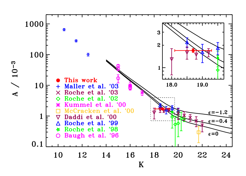
Figure 2: Amplitude $A$ of the angular correlation function $w(\theta)$ as a function of $K$-band magnitude. We have plotted our survey at an effective $K=18.7$ mag. Existing data comes from Baugh et al. (1996); Roche et al. (1998, 1999); Daddi et al. (2000); McCraken et al. (2000); Kümmel and Wagner (2000); Roche et al. (2002, 2003); Maller et al. (2003). All data have fixed $\gamma=1.8$ except for those of Maller et al. (2003) who found $\gamma\approx 1.76$, depending on scale. The lines are the evolving models of Roche et al. (2003), with stable ($\epsilon=0$), co-moving $\epsilon=-1.2$ and intermediate $\epsilon=-0.4$ clustering. An expanded view of our new measurement is shown in the inset.

In Figure 2 we compare our amplitude with that from various $K$-band surveys. Our errors are much smaller than existing measurements in these range but there is a very good agreement, the main issue is the uncertainty in how to compare the $K$- and $L$-band limits.

Roche et al. (2003) have modeled the clustering of $K$-band sources with the auto-correlation function evolving as

$$\xi(r,z)=\left(r/r_{0}\right)^{-\gamma}\left(1+z\right)^{-(3+\epsilon)}$$

Setting the local $r_{0}=5.85h^{-1}$ Mpc (Cabanac, de Lapparent and Hickson, 2000) and using their own model for the redshift distribution, they estimate the angular correlation function as shown in Figure 2. We find good agreement with their stable clustering, $\epsilon=0$, model. Interestingly their model appears to over-predict the strength of the 2MASS clustering (Maller et al., 2003), though these data have been plotted with the slightly shallower best-fit slopes $\gamma\approx 1.76$.

3.2 Estimation of 3D clustering

We can use our two-dimensional clustering measurement to infer the three-dimensional clustering statistics. To do this we need to know the shape of the redshift distribution $dN/dz(z)$. In the absence of spectroscopic redshifts or photometric redshifts for all our sources we use the model of Xu et al. (2003) to estimate the redshift distribution.

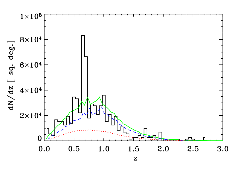
Figure 3: The redshift distribution from the K20 sample (Cimatti et al., 2002) compared with the model of Xu et al. (2003). The model starbursts are shown in blue (middle curve), spheroids in red (lower curve) and total counts in green (upper curve). We have normalized the total counts in the model to the total number of sources in the K20 sample (dividing by a factor of two).

We know that this model over predicts the 3.6 µm number counts (Lonsdale et al., 2004), so it is important to demonstrate that this model can nevertheless predict the shape of the redshift distribution. In Figure 3 we compare the model with the observed redshift distribution from the K20 sample (Cimatti et al., 2002). The shape is a reasonable fit. The median redshift of the K20 sample is $z_{\rm med}=0.74$; for our model starbursts and spirals we find $z_{\rm med}=0.92$, while for the spheroids $z_{\rm med}=0.86$, and the model as a whole has $z_{\rm med}=0.91$. The median redshift of the K20 sample is biased by a sharp peak at $z\simeq 0.74$, which is presumably an artifact of clustering. So although the K20 sample has a slightly lower median $z$ than our model, we regard the approximate agreement between the redshift distributions in Figure 3 as reasonable confirmation of the model.

Using this model we estimate that our $S_{3.6}\geq 32$ $\mu$Jy sample has a median redshift of $z_{\rm med}\approx 0.75$. If the median redshift is lower than this, say by a factor of 0.8 as in the K20 comparison above then the median redshift might be $z_{\rm med}\approx 0.6$.

Using the Limber’s equation (Limber, 1953) inversion technique adopted by Gonzalez-Solares et al. (2004), which uses a redshift distribution parameterized by the median redshift, we estimate the real-space correlation function $\xi(r)=(r/r_{0})^{1.8}$ for our combined sample and find $r_{0}=4.4\pm 0.1h^{-1}$ Mpc. The results for individual fields are shown in Table 1. Adopting the lower redshift, $z_{\rm med}=0.6$, this drops to $r_{0}=3.3\pm 0.1h^{-1}$ Mpc. For comparison the correlation function of quasars in the range $0.3<z<2.9$ has $r_{0}=3.99^{+0.34}_{-0.28}h^{-1}$ Mpc, with $\gamma=1.58^{+0.09}_{-0.10}$ (Croom et al., 2001) and hyper-luminous infrared galaxies also have a clustering strength similar to AGN at $z\sim 0.7$ (Farrah et al., 2004). The uncertainty in our correlation function is clearly dominated by our uncertainties in the redshift distribution and emphasizes the need to establish the redshift distribution of the SWIRE galaxies.

3.3 Conclusions and future work

We have performed the first clustering analysis on the SWIRE survey. We have a very strong detection of clustering with amplitude similar to $K$-band surveys but with smaller errors. We are thus consistent with an existing phenomenological model of $K$-band selected galaxies $\xi(r,z)=\left(r/r_{0}\right)^{-\gamma}\left(1+z\right)^{-3}$. Physically this model could be interpreted as stable clustering, i.e. that galaxies have broken free from the Hubble expansion, though this seems implausible on large scales. However, since $K$-band surveys sample different galaxies at different redshifts the interpretation of the phenomenological model is not this straightforward. Now that we have high quality data in the rest-frame $K$ at high redshift we need phenomenological models specifically designed to interpret these.

When we have a larger survey area available, and detailed selection functions, we will be able to extend the analysis to our completeness limit, which is fainter by a factor of nearly 10 in flux (or 2.5 magnitudes). We will then be able to subdivide our sample by flux and explore the evolution of clustering in much more detail. We will investigate the excess clustering seen on smaller angular scales, and we will also explore the clustering in the longer wavelength IRAC bands and the relative clustering of star-forming galaxies and passively evolving systems, thus gaining insights into the nature of galaxy bias.

Table 1: Parameterized $w(\theta)$ estimated from each of our sub samples.

Sample	Area	$N_{\rm gals}$	$N_{\rm stars}$	$A(\gamma=1.8)$	$A$	$\gamma$	$r_{0}(z_{\rm med}=0.75)$	$r_{0}(z_{\rm med}=0.6)$
	[sq. deg.]			$[10^{-3}]$	$[10^{-3}]$		$[h^{-1}{\rm Mpc}]$	$[h^{-1}{\rm Mpc}]$
Lockman (optical)	0.3	2115	872	$2.7\pm 0.5$	$1.2\pm 1.3$	$1.97\pm 0.25$	$5.5\pm 0.5$	$4.3\pm 0.5$
Lockman full tile	0.4	3685	1551	$2.0\pm 0.3$	$1.0\pm 1.0$	$1.95\pm 0.23$	$4.6\pm 0.4$	$3.7\pm 0.3$
ELAIS N1 tile_2_2	0.8	8677	4163	$1.7\pm 0.2$	$0.5\pm 0.3$	$2.06\pm 0.14$	$4.2\pm 0.3$	$3.3\pm 0.3$
ELAIS N1 tile_3_2	0.8	8472	4272	$1.7\pm 0.2$	$0.9\pm 0.6$	$1.95\pm 0.16$	$4.2\pm 0.3$	$3.3\pm 0.3$
Combined sample	2.0	20834	9986	$1.7\pm 0.1$	$0.6\pm 0.3$	$2.03\pm 0.10$	$4.4\pm 0.1$	$3.3\pm 0.1$

Column 3 is the number of galaxies included in each sample, and column 4 is the number of stars that were rejected. $w(\theta)$ is modeled as $w(\theta)=A\theta^{1-\gamma}$, with $\theta$ measured in degrees. Column 5 has $\gamma=1.8$ fixed, while columns 6 and 7 are the results for a free fit. Columns 8 and 9 are estimates of the strength of the correlation function $\xi(r)=(r/r_{0})^{1.8}$ assuming a median redshift of $z=0.75$ and $z=0.6$ respectively. The Lockman (optical) sample is a subset of the Lockman full tile and is not included in the combined sample.

Figure 1: The angular correlation function $w(\theta)$ in each of our fields. The best-fitting power law with fixed slope is shown as a solid line. This power law is the same for both ELAIS N1 tiles, $w(\theta)=0.0017\,(\theta/{\rm deg})^{-0.8}$, and this is plotted as a dotted line in the other panels for reference.

References

- Baugh et al. (1996) Baugh C. M., Gardner J. P., Frenk C. S., Sharples R.M ., 1996, MNRAS, 283, L15.
- Bennett et al. (2003) Bennett, C. L., et al. 2003, ApJS, 148, 1
- Benson et al. (2001) Benson A. J., Frenk C. S., Baugh C. M., Cole S., Lacey C. G., 2001, MNRAS, 327, 1041
- Cabanac, de Lapparent and Hickson (2000) Cabanac A., de Lapparent V., Hickson P., 2000, A&A, 364, 349.
- Cimatti et al. (2002) Cimatti A., et al. 2002, A&A, 391, L1
- Croom et al. (2001) Croom S.M, Shanks T., Boyle B.J., Smith R.J., Miller L., Loaring N.S., Hoyle F. 2001, MNRAS, 325, 483
- Cutri et al. (2003) Cutri, R. M., et al., 2003, Explanatory Supplement to the 2MASS All Sky Data Release, http://www.ipac.caltech.edu/2mass/releases/allsky/doc/explsup.html
- Daddi et al. (2000) Daddi E., Cimatti A., Pozzetti L., Hoekstra H., Röttgering, H., Renzini A., Zamorani G., Mannucci F, 2000, A&A, 361, 535.
- Farrah et al. (2004) Farrah et al., 2004, MNRAS, 349, 518
- Gonzalez-Solares et al. (2004) Gonzalez-Solares et al., 2004, MNRAS, (in press) astro-ph/0312451
- Jarrett et al. (1994) Jarrett, Jarrett, T. H., Dickman, R. L., & Herbst, W. 1994, ApJ, 424, 852
- Kümmel and Wagner (2000) Kümmel M. W., and Wagner S. J. 2000, A&A, 353, 867
- Landy and Szalay (1993) Landy S. D., and Szalay A. S., 1993, ApJ, 412, 64
- Limber (1953) Limber, D. N. 1953, ApJ, 117, 134
- Lonsdale et al. (2004) Lonsdale C., et al. 2004, ApJS, (this issue)
- Lonsdale et al. (2003) Lonsdale C., et al. 2003, PASP, 115, 897
- Maddox et al. (1990) Maddox, S. J., Efstathiou, G., Sutherland, W. J., & Loveday, J. 1990, MNRAS, 242, 43P
- Maller et al. (2003) Maller A. H., McIntosh D. H., Katz N., and Wessinberg M. D., 2003, astro-ph/0304005
- McCraken et al. (2000) McCracken H., Shanks T., Metcalfe N., Fong R., Campos A., 2000, MNRAS, 318, 913.
- Peebles (1980) Peebles P.J.E., 1980, The Large-Scale Structure of the Universe, Princeton University Press.
- Roche et al. (2002) Roche N., Almaini O., Dunlop J., Ivison R. J., Willott C. J., 2002, MNRAS, 337, 1282.
- Roche et al. (2003) Roche, N., Dunlop, J., Almaini, O., 2003, MNRAS, 346, 803
- Roche et al. (1999) Roche, N., Eales, S., Hippelein, H., Willott, C. J., 1999, MNRAS, 306, 538.
- Roche et al. (1998) Roche, N., Eales, S., Hippelein, H., 1998, MNRAS, 295, 946.
- Rowan-Robinson et al. (2004) Rowan-Robinson, M., et al., 2004, ApJS, (this issue)
- Surace et al. (2004) Surace, J., et al., 2004, in preparation
- Xu et al. (2003) Xu, C. K., Lonsdale, C. J., Shupe, D. L., Franceschini, A., Martin, C., and Schiminovich, D., 2003, ApJ, 587, 90