The Angular Power Spectrum of the First-Year WMAP Data Reanalysed

Abstract

We measure the angular power spectrum of the WMAP first-year temperature anisotropy maps. We use SpICE (Spatially Inhomogeneous Correlation Estimator) to estimate $C_{\ell}$’s for multipoles $\ell=2-900$ from all possible cross-correlation channels. Except for the map-making stage, our measurements provide an independent analysis of that by Hinshaw et al. (2003a). Despite the different methods used, there is virtually no difference between the two measurements for $\ell\lower 2.15277pt\hbox{$\;\buildrel<\over{\sim}\;$}700$ ; the highest $\ell$’s are still compatible within $1-\sigma$ errors. We use a novel intra-bin variance method to constrain $C_{\ell}$ errors in a model independent way. Simulations show that our implementation of the technique is unbiased within 1% for $\ell\lower 2.15277pt\hbox{$\;\buildrel>\over{\sim}\;$}100$. When applied to WMAP data, the intra-bin variance estimator yields diagonal errors $\sim 10\%$ larger than those reported by the WMAP team for $100<\ell<450$. This translates into a 2.4 $\sigma$ detection of systematics since no difference is expected between the SpICE and the WMAP team estimator window functions in this multipole range. With our measurement of the $C_{\ell}$’s and errors, we get $\chi^{2}/d.o.f.=1.042$ for a best-fit $\Lambda$CDM model, which has a 14 % probability, whereas the WMAP team (Spergel et al., 2003) obtained $\chi^{2}/d.o.f.=1.066$, which has a 5 % probability. We assess the impact of our results on cosmological parameters using Markov Chain Monte Carlo simulations. From WMAP data alone, assuming spatially flat power law $\Lambda$CDM models, we obtain the reionization optical depth $\tau=0.145\pm 0.067$, spectral index $n_{s}=0.99\pm 0.04$, Hubble constant $h=0.67\pm 0.05$, baryon density $\Omega_{b}h^{2}=0.0218\pm 0.0014$, cold dark matter density $\Omega_{cdm}h^{2}=0.122\pm 0.018$, and $\sigma_{8}=0.92\pm 0.12$, consistent with a reionization redshift $z_{re}=16\pm 5$ (68 $\%$ CL).

1 Introduction

The Wilkinson Microwave Anisotropy Probe satellite (WMAP) has provided the clearest view of the primordial universe to date. Its unprecedented high sensitivity and spatial resolution resulted in a unique set of cosmic microwave background (CMB) radiation maps with close to full sky coverage and uniformly high quality. As a result, fundamental cosmological parameters can be constrained to the highest precision ever. Thorough analysis of this dataset (Bennett et al., 2003) yielded a cosmic variance limited measurement of the angular power spectrum, $C_{\ell}$’s, of the CMB temperature anisotropy for multipoles $\ell\lower 2.15277pt\hbox{$\;\buildrel<\over{\sim}\;$}350$ (Hinshaw et al. (2003a); hereafter H03). This confirmed and improved measurements from previous experiments (e.g., Miller et al. (1999); de Bernardis et al. (2000); Hanany et al. (2000); Halverson et al. (2002); Mason et al. (2003); Scott et al. (2003); Benoît et al. (2003)). The acoustic peak structure revealed by the WMAP temperature and polarization power spectra provided strong observational support to inflation and constrained viable cosmological scenarios to the domain of flat $\Lambda$CDM models and its close variants.

Considering the importance of these results, our principal aim is to estimate the angular power spectrum in a completely independent way in the full range of multipoles probed by WMAP, $2\leq\ell\leq 900$, and systematically compare results to H03. Our $C_{\ell}$ estimation pipeline is based on SpICE (Spatially Inhomogeneous Correlator Estimator; Szapudi et al., 2001a, b), a quadratic estimator based on correlation functions. SpICE performs edge corrections and heuristic minimum variance weighting in pixel space to produce nearly optimal results. Our fast HEALPix implementation of SpICE scales as ${\rm{\cal O}(N^{3/2})}$ (${\rm N}$ is number of pixels).

2 Power Spectrum Estimation

Our estimation methodology closely follows that of H03, but adapted to our technique:

Step 1: We use the foreground cleaned intensity maps for the 3 highest frequency bands Q, V & W downloaded from the LAMBDA website . Strong diffuse Galactic emission and resolved point sources are masked out using the Kp0 and Kp2 masks, that leaves $76.8\%$ and $85.0\%$ of the sky useful for cosmological analyses, respectively. Monopole $\ell=0$ and dipole $\ell=1$ terms are also removed from non-masked pixels.

Step 2: Power-spectrum estimation is performed via SpICE: we compute the cross-correlations from 28 different pairs of channels constructed from the 8 “differencing assemblies” (DAs) Q1 through W4. Noise correlation among different channels is negligible, therefore our cross-power estimator is unbiased with respect to the noise (see e.g., H03). Like H03, we implement an heuristic $\ell$-dependent pixel noise weighting scheme that minimizes errors: we use flat weights (mask weight only) for $\ell<200$, inverse pixel noise variance for $\ell>450$, and a transitional inverse rms noise weight in the intermediate range $200<\ell<450$.

Step 3: A model for the power spectrum for unresolved extragalactic radio sources is subtracted from the cross-power spectrum of each channel. We implement the model given in §3.1 of H03.

Step 4: $C_{\ell}$’s from different channels are optimally combined using an inverse noise weighting, with DA sensitivities as described in the LAMBDA website. All channels are included, except for those in Q-band that are only used in the intermediate $\ell$-range. This helps minimizing galactic contamination at low $\ell$ and the window function cut-off at the highest multipoles.

Step 5: Our quadratic estimator is defined in pixel space, where mask effects can be easily corrected for (cf. Szapudi et al., 2001a). The two point correlation function is then transformed into harmonic space via Gauss-Legendre quadrature to obtain the $C_{\ell}$’s deconvolved from the window function of the experiment. Symmetrized non-Gaussian beam transfer profiles (Page et al., 2003) and pixel window functions are corrected for in $\ell$-space.

3 Principal Results

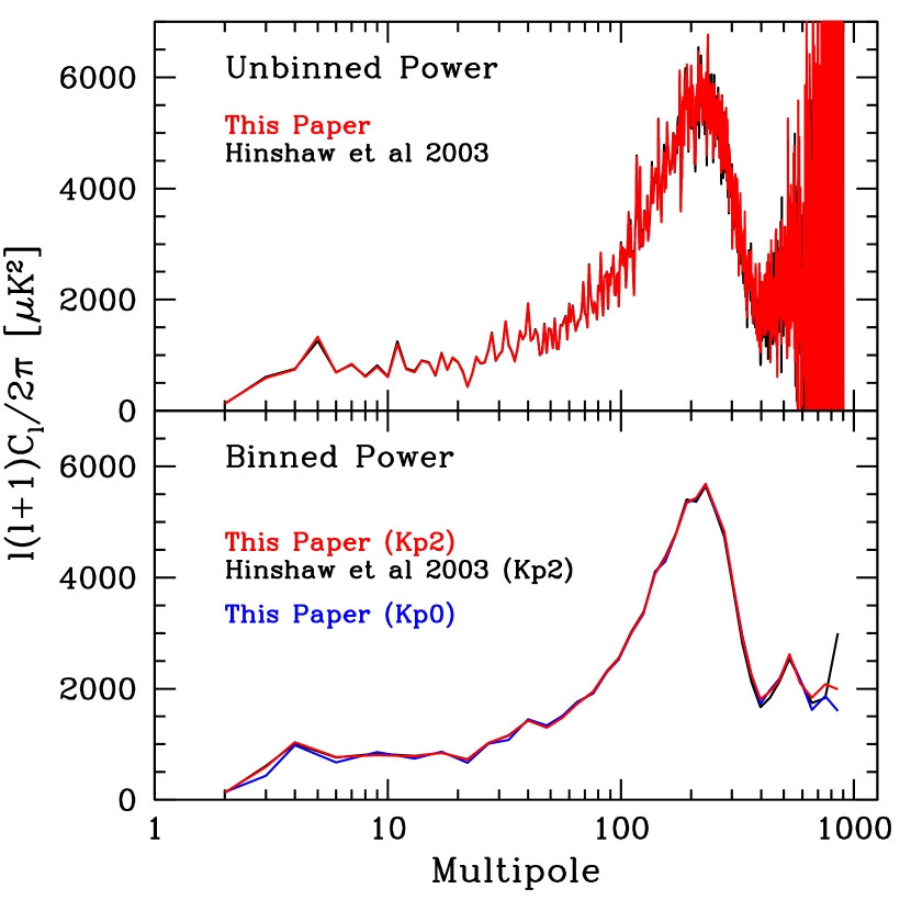
Figure 1: WMAP angular power spectrum of the 1st-year temperature anisotropy data. Upper panel: Measurement for individual multipoles (red line) using the Kp2 sky cut. Results from by H03 are also shown (black line, nearly indistinguishable from red). The agreement is excellent for most $\ell$’s. Lower panel: Binned power spectrum for two different sky cuts, Kp2 (red) & Kp0 (blue). We find excellent agreement with H03 (black line) for all multipoles $\ell\lower 2.15277pt\hbox{$\;\buildrel<\over{\sim}\;$}700$ and a slightly different amplitude for the highest $\ell$’s.

Figure 1 shows the angular power spectrum of WMAP, $\Delta T^{2}_{\ell}\equiv\ell(\ell+1)C_{\ell}/2\pi$, in $\mu$K² units, measured with SpICE. Upper panel shows the power spectrum for individual multipoles, using Kp2 sky cut. Our measurement (red line) is in excellent agreement with H03 (black line), multipole by multipole. In particular, for the quadrupole and octopole we find $\Delta T^{2}_{2}\sim 135\mu$K² and $\Delta T^{2}_{3}\sim 591\mu$K², respectively (H03 get $\sim 123\mu$K² and $\sim 612\mu$K²). For the highest ${\ell}$’s we find slightly different amplitudes than H03, but consistent at the 1-$\sigma$ level.

For the most part, we observe no systematic dependence of the measured $C_{\ell}$’s on the sky cut (see difference between red and blue lines in bottom panel of Figure 1). However, using Kp0 instead of Kp2 yields a $15\%$ lower amplitude of the octopole $\ell=3$ and a $15-20\%$ smaller amplitudes for the 3 highest band-powers centered at $\ell_{\rm eff}\sim 660,750,850$. This effect might be due to imperfect foreground removal and/or the intrinsic estimator variance due to finite volume and edge effects. We estimated the dispersion in a set of WMAP simulations with Kp0 & Kp2 sky cuts to be of the same order as the measured differences in the $C_{\ell}$’s of the data. On the other hand, the cross-correlation amplitude between the clean WMAP maps and the best fit foreground templates is at the 5% and 10% level of the WMAP $C_{\ell}$’s for the lowest and highest $\ell$’s, respectively. We thus conclude that sample variance due to sky coverage can account for most of the observed difference in the $C_{\ell}$’s, while residual foreground contamination is always subdominant. The low level of systematics in Kp2, and the increased statistical errors due to the decreased sky fraction left by Kp0, motivate us to adopt Kp2 (as in H03) for the best estimate of the $C_{\ell}$’s.

4 Error Estimation

In order to estimate the covariance of our $C_{\ell}$’s, we generated MC simulations of the CMB sky and instrument noise for each of the 8 DA’s (Q1 through W4). We used the running index $\Lambda$CDM model that best fits a combination of WMAP, CBI & ACBAR data (denoted WMAPext in Spergel et al. (2003)). Maps were convolved with the symmetric (non-Gaussian) beam transfer function for each DA (Page et al., 2003). As for the noise simulations, we downloaded 100 sky maps per DA from the LAMBDA website. These simulate 1 full year of flight instrument noise and they include all known radiometric effects (Hinshaw et al., 2003b; Jarosik et al., 2003). Simulations were analyzed in exactly the same way as the data (see §2). All in all, we have constrained the errors from $1500$ measurements in MC simulations (combining cross spectra using 100 MC’s for each of the 6 highest frequency DA’s V1 through W4) for the multipole ranges $\ell<200$ and $\ell>450$, and $2800$ measurements (combining cross-spectra using 100 MC’s from each of the 8 DA’s Q1 through W4) for the intermediate $\ell$-range $200<\ell<450$.

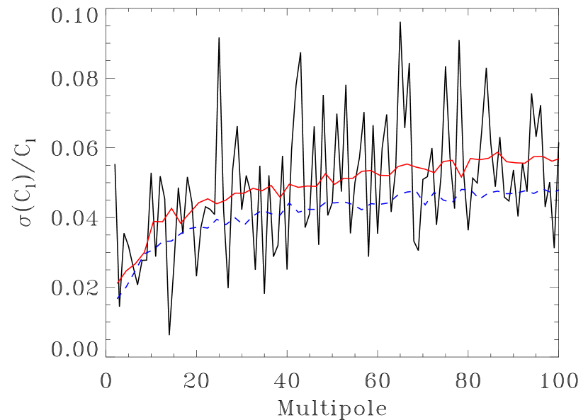
Figure 2: Errorbars estimated from uncorrelated (dash line) and correlated noise (solid smooth line) are shown. The spiky solid line shows the variance of the $C_{\ell}$’s among the data channels, what should depend on noise only. The Monte Carlo simulations with non-uniform noise appear to describe well the mean rms errors.

For multipoles $\ell<350$, errors in the WMAP power spectrum are dominated by cosmic or sample variance (see H03) and the noise only contributes at the few percent level. Figure 2 displays the noise contribution to the relative errors at low multipoles, $\ell\lower 2.15277pt\hbox{$\;\buildrel<\over{\sim}\;$}100$. Correlated noise simulation results are displayed (smooth solid line) along with results from uncorrelated noise simulations (dashed line). The latter tends to underestimate errors by $\sim 1\%$. Alternatively the noise level can be estimated from the data rms dispersion among the WMAP channels used (oscillating solid line). These results are in excellent agreement with H03 (cf. lower panel in their Figure 4).

At higher $\ell$’s pixel noise and systematic effects (e.g., beam and mode coupling, residual foregrounds) increasingly dominate the errors. MC methods assume detailed knowledge of all such effects. To provide a model independent check of the errors, we introduce a novel technique that allows estimating errors directly from the data: the intra-bin variance (IBV) method. IBV estimates the variance of a given $C_{\ell}$ from the rms dispersion in a bin $\rm B_{\ell}$ centered on $\ell$. The bin-width ${\Delta\ell}$ is a matter of practical consideration, balancing variance and bias. More precisely, our estimator for $\sigma(C_{\ell})$ reads

$$\sigma^{2}(C_{\ell})={1\over{\Delta{\ell}-1}}\sum_{{\ell}^{\prime}\in{\rm B_{\ell}}}({\Delta C_{{\ell}^{\prime}}}-{\langle{\Delta C_{\ell}\rangle}})^{2}$$ (1)

where $\langle{\Delta C_{\ell}}\rangle=1/\Delta{\ell}\sum_{{\ell}^{\prime}\in\rm B_{\ell}}\Delta C_{{\ell}^{\prime}},\,$ $\Delta C_{\ell}={\bar{C}_{\ell}}-C^{\rm th}_{\ell}$, ${\bar{C_{\ell}}}$ is the mean of the measured $C_{\ell}$’s over channels, and $C^{\rm th}_{\ell}$ is our best guess for the data mean using a theoretical $\Lambda$CDM model. The latter is subtracted to decrease the bias due to the slope of the angular power spectrum. We used $C^{\rm th}_{\ell}$ from the WMAP best-fit running index $\Lambda$CDM model (Spergel et al., 2003), although this is not critical: no baseline subtraction only biases at a few percent level. By construction, IBV should not be used to obtain errors with high resolution but to assess the overall level of errors in a range of $\ell$’s, typically larger than $\Delta\ell$.

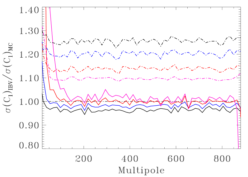
Figure 3: Solid lines show the ratio of intra-bin variance (IBV) to Monte Carlo errors measured in WMAP simulations. At $\ell\simeq 300$ lines correspond to $\Delta\ell=6,9,18,36$ (bottom up). The third line ($\Delta\ell=18$) is unbiased for $\ell>100$. Upper dotted lines (in reverse order to solid lines) correspond to the relative rms error on the estimated IBV errors (e.g., in the convention used, $1.15$ means $15\%$ error).

Figure 3 shows the ratio between the mean IBV rms dispersion to the usual MC rms dispersion, both estimated from $\sim 3000$ WMAP simulations of CMB signal and correlated noise. Narrow bins yield slightly biased (under-)estimates of the MC error at few percent level, possibly due to small mode-to-mode couplings. IBV method with $\Delta\ell=18$ yields unbiased estimates of the error for WMAP simulations at the 1% level for $\ell\lower 2.15277pt\hbox{$\;\buildrel>\over{\sim}\;$}100$. Doubling $\Delta\ell$ introduces a slight high bias and significant edge effects for low $\ell$’s that could be caused by the residual slope of the $C_{\ell}$’s. The unbiased bin-width, $\Delta\ell=18$, with $15\%$ variance is our choice for the WMAP error estimation.

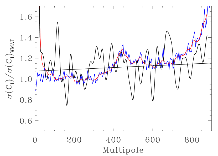
Figure 4: Ratio of measured errors vs. published WMAP errors (Verde et al., 2003; Hinshaw et al., 2003b; Kogut et al., 2003). The noisy blue line and smooth red line through the latter show the usual MC dispersion and the average IBV error respectively, for the same set of simulations. The large amplitude oscillating black line shows the IBV estimator applied to the WMAP data. The IBV method detects 8-15% larger errors than the published ones. A conservative IBV error estimation is depicted by the solid straight line obtained from a linear least square fit.

Figure 4 displays the WMAP data diagonal errorbars computed with the IBV method (spiky solid line) compared to the previously published diagonal errors (Verde et al. (2003),Hinshaw et al. (2003b),Kogut et al. (2003)). The largest IBV errors appear to correlate well with the outliers of the data $C_{\ell}$’s with respect to the best-fit $\Lambda$CDM model (see Figure 3 in Spergel et al. (2003)), suggesting that our IBV estimator is closely related to a diagonal $\chi^{2}$ test. It is clear that the mean overall error is higher than originally estimated (otherwise the IBV curve would fluctuate around unity). The simplest and most conservative interpretation of our results yields a monotonic error increase with respect to the WMAP team diagonal errors of the form, $\sigma(C_{\ell})_{IBV}/\sigma(C_{\ell})_{WMAP}\simeq 1.08+8.5\cdot 10^{-5}({\ell}-100)$ for $\ell>100$ (straight solid line in Figure 4). This smooth prediction results from a least squares minimization to the IBV curve (large amplitude oscillating line in Figure 4). Note that for $\ell>450$, the error excess is consistent with the errors estimated from MC simulations with correlated instrument noise (see noisy line in Figure 4 growing from left to right).

In the range $100<\ell<450$ the mean error level is incompatible with both MC simulations that include correlated noise and the WMAP team published errors: given that there are approximately 16 independent $\Delta{\ell}$ bins, with an intrinsic 15 % error each, and that the mean error excess is 9 % in this $\ell$-range, this amounts to a 2.4 $\sigma$ detection of the error excess. We have checked that using the $C_{\ell}$’s measured by Hinshaw et al. (2003a) yields comparable IBV errors in this multipole range. The excellent $\ell$-by-$\ell$ agreement between the SpICE and WMAP team’s measurement of the $C_{\ell}$’s (see Figure 1) indicates that both estimators window functions are virtually identical in this regime, and thus the observed error excess points to systematics unaccounted for in the WMAP team analyses. For $\ell>450$ the interpretation is less clear as there are hints that both window functions might be slightly different (see lower panel in Figure 1). Such differences might arise in the practical implementation of the estimators. We also estimate a $\sim 5\%$ correlated noise contribution at $\ell<100$ (see Figure 2), that was neglected in previous likelihood analyses. A more robust assessment of errors is provided below using the full $\chi^{2}$ test, where off-diagonal terms are also taken into account following Eq.(15) in Verde et al. (2003).

5 Discussion: Cosmological Parameters

We investigate the implications of our measurements using a Bayesian analysis of cosmological parameter estimation. We use CosmoMC, a Markov Chain Monte Carlo (MCMC) implementation (Lewis and Bridle, 2002) based on CAMB (Lewis et al. (2000); see also CMBFAST, Seljak and Zaldarriaga (1996)). In order to allow direct comparison with Spergel et al. (2003), we focus on the simplest 6-parameter cosmological model consistent with the WMAP temperature and cross-polarization data. Following Verde et al. (2003), we assume a set of flat $\Lambda$CDM models with radiation, baryons, cold dark matter and cosmological constant. Primordial fluctuations are taken to be adiabatic and Gaussian with a power-law power spectrum. We use the physical dark matter $\Omega_{cdm}h^{2}$ and baryon $\Omega_{b}h^{2}$ densities, the reionization optical depth $\tau$, the scalar spectral index $n_{s}$, the normalized Hubble constant $h$, and the dark matter power spectrum normalization $\sigma_{8}$ (Kosowsky et al., 2002). We estimate paramaters by combining 4 independent chains with 30000 accepted points each, and use the 6 paramater covariance matrix as proposal density from precomputed runs. This yields an excellent convergence-mixing Gelman & Rubin statistic $R-1\lower 2.15277pt\hbox{$\;\buildrel<\over{\sim}\;$}0.02$ for all cases studied.

Table 1: Best Fit Parameters for Power Law $\Lambda$ CDM^a

	SpICE $C_{\ell}$’s	WMAP $C_{\ell}$’s
	IBV Errorsb	Standard Errorsc
$\tau$	$0.145\pm 0.067$	$0.151\pm 0.069$
$n_{s}$	$0.99\pm 0.04$	$0.99\pm 0.04$
$h$	$0.67\pm 0.05$	$0.70\pm 0.05$
$\Omega_{b}h^{2}$	$0.0218\pm 0.0014$	$0.0234\pm 0.0013$
$\Omega_{cdm}h^{2}$	$0.122\pm 0.018$	$0.123\pm 0.017$
$\sigma_{8}$	$0.92\pm 0.12$	$0.92\pm 0.11$
$\chi^{2}_{eff}/dof$	1398.8/1342	1428.7/1342

Table 1 summarizes our results. Imposing the prior $\tau<0.3$, we find best fit values matching those of Spergel et al. (2003). In particular we obtain a $\chi^{2}/d.o.f.=1.042$ (i.e. it has a 14 % probability) for the best-fit model (see first column in Table 1), which is a slightly better fit to the data than that of Spergel et al. (2003), $\chi^{2}/d.o.f.=1.066$ (i.e. 5 % probability). Our $h$ and $\tau$ are slightly lower but still consistent at the $1-\sigma$ level. This is more significant for our estimates of the $C_{\ell}$’s and errors (see first column in Table 1). In particular, our measurement $\Omega_{b}h^{2}=0.0218\pm 0.0014$ agrees with that from the latest BBN results $\Omega_{b}h^{2}=0.022\pm 0.002$ (Cyburt et al., 2003; Vangioni-Flam et al., 2003; Cuoco et al., 2003). We have checked that relaxing the $\tau$ prior yields larger values of $\tau=0.19\pm 0.12$ (cf. Tegmark et al., 2004). Our main results (see first column in Table 1) are in excellent agreement with the best-fit values from WMAP+SDSS (Tegmark et al., 2004), and suggest a redshift of (abrupt) reionization $z_{re}=16\pm 5$ ($68\%$ CL). Data products and additional plots from this work can be found at http://www.ifa.hawaii.edu/cosmowave/wmap.html

We thank an anonymous referee for insightful comments, Jun Pan for help and discussions, Olivier Dore, Hans K. Eriksen, Eiichiro Komatsu for useful comments, and Antony Lewis for help with CosmoMC. We acknowledge extensive use of the Legacy Archive for Microwave Background Data Analysis (LAMBDA). Support for LAMBDA is provided by the NASA Office of Space Science. Some of the results in this paper have been derived using HEALPix (Górski et al., 1998). This research was supported by NASA through ATP NASA NAG5-12101 and AISR NAG5-11996, as well as by NSF grants AST02-06243 and ITR 1120201-128440.

References

- Hinshaw et al. (2003a) G. Hinshaw, D. N. Spergel, L. Verde, R. S. Hill, S. S. Meyer, C. Barnes, C. L. Bennett, M. Halpern, N. Jarosik, A. Kogut, et al., ApJS 148, 135 (2003a).
- Spergel et al. (2003) D. N. Spergel, L. Verde, H. V. Peiris, E. Komatsu, M. R. Nolta, C. L. Bennett, M. Halpern, G. Hinshaw, N. Jarosik, A. Kogut, et al., ApJS 148, 175 (2003).
- Bennett et al. (2003) C. L. Bennett, M. Halpern, G. Hinshaw, N. Jarosik, A. Kogut, M. Limon, S. S. Meyer, L. Page, D. N. Spergel, G. S. Tucker, et al., ApJS 148, 1 (2003).
- Miller et al. (1999) A. D. Miller, R. Caldwell, M. J. Devlin, W. B. Dorwart, T. Herbig, M. R. Nolta, L. A. Page, J. Puchalla, E. Torbet, and H. T. Tran, ApJ 524, L1 (1999).
- de Bernardis et al. (2000) P. de Bernardis, P. A. R. Ade, J. J. Bock, J. R. Bond, J. Borrill, A. Boscaleri, K. Coble, B. P. Crill, G. De Gasperis, P. C. Farese, et al., Nature 404, 955 (2000).
- Hanany et al. (2000) S. Hanany, P. Ade, A. Balbi, J. Bock, J. Borrill, A. Boscaleri, P. de Bernardis, P. G. Ferreira, V. V. Hristov, A. H. Jaffe, et al., ApJ 545, L5 (2000).
- Halverson et al. (2002) N. W. Halverson, E. M. Leitch, C. Pryke, J. Kovac, J. E. Carlstrom, W. L. Holzapfel, M. Dragovan, J. K. Cartwright, B. S. Mason, S. Padin, et al., ApJ 568, 38 (2002).
- Mason et al. (2003) B. S. Mason, T. J. Pearson, A. C. S. Readhead, M. C. Shepherd, J. Sievers, P. S. Udomprasert, J. K. Cartwright, A. J. Farmer, S. Padin, S. T. Myers, et al., ApJ 591, 540 (2003).
- Scott et al. (2003) P. F. Scott, P. Carreira, K. Cleary, R. D. Davies, R. J. Davis, C. Dickinson, K. Grainge, C. M. Gutiérrez, M. P. Hobson, M. E. Jones, et al., MNRAS 341, 1076 (2003).
- Benoît et al. (2003) A. Benoît, P. Ade, A. Amblard, R. Ansari, É. Aubourg, S. Bargot, J. G. Bartlett, J.-P. Bernard, R. S. Bhatia, A. Blanchard, et al., A&A 399, L19 (2003).
- Szapudi et al. (2001a) I. Szapudi, S. Prunet, D. Pogosyan, A. S. Szalay, and J. R. Bond, ApJ 548, L115 (2001a).
- Szapudi et al. (2001b) I. Szapudi, S. Prunet, and S. Colombi, ApJ 561, L11 (2001b).
- Hivon et al. (2002) E. Hivon, K. M. Górski, C. B. Netterfield, B. P. Crill, S. Prunet, and F. Hansen, ApJ 567, 2 (2002).
- Page et al. (2003) L. Page, C. Barnes, G. Hinshaw, D. N. Spergel, J. L. Weiland, E. Wollack, C. L. Bennett, M. Halpern, N. Jarosik, A. Kogut, et al., ApJS 148, 39 (2003).
- Hinshaw et al. (2003b) G. Hinshaw, C. Barnes, C. L. Bennett, M. R. Greason, M. Halpern, R. S. Hill, N. Jarosik, A. Kogut, M. Limon, S. S. Meyer, et al., ApJS 148, 63 (2003b).
- Jarosik et al. (2003) N. Jarosik, C. Barnes, C. L. Bennett, M. Halpern, G. Hinshaw, A. Kogut, M. Limon, S. S. Meyer, L. Page, D. N. Spergel, et al., ApJS 148, 29 (2003).
- Verde et al. (2003) L. Verde, H. V. Peiris, D. N. Spergel, M. R. Nolta, C. L. Bennett, M. Halpern, G. Hinshaw, N. Jarosik, A. Kogut, M. Limon, et al., ApJS 148, 195 (2003).
- Kogut et al. (2003) A. Kogut, D. N. Spergel, C. Barnes, C. L. Bennett, M. Halpern, G. Hinshaw, N. Jarosik, M. Limon, S. S. Meyer, L. Page, et al., ApJS 148, 161 (2003).
- Lewis and Bridle (2002) A. Lewis and S. Bridle, Phys. Rev. D66, 103511 (2002), astro-ph/0205436.
- Lewis et al. (2000) A. Lewis, A. Challinor, and A. Lasenby, Astrophys. J. 538, 473 (2000), astro-ph/9911177.
- Seljak and Zaldarriaga (1996) U. Seljak and M. Zaldarriaga, Astrophys. J. 469, 437 (1996), astro-ph/9603033.
- Kosowsky et al. (2002) A. Kosowsky, M. Milosavljevic, and R. Jimenez, Phys. Rev. D 66, 063007 (2002).
- Cyburt et al. (2003) R. H. Cyburt, B. D. Fields, and K. A. Olive, Physics Letters B 567, 227 (2003).
- Vangioni-Flam et al. (2003) E. Vangioni-Flam, A. Coc, and M. Cassé, Nuclear Physics A 718, 389 (2003).
- Cuoco et al. (2003) A. Cuoco, F. Iocco, G. Mangano, G. Miele, O. Pisanti, and P. D. Serpico, ArXiv Astrophysics e-prints (2003), astro-ph/0307213.
- Tegmark et al. (2004) M. Tegmark, M. A. Strauss, M. R. Blanton, K. Abazajian, S. Dodelson, H. Sandvik, X. Wang, D. H. Weinberg, I. Zehavi, N. A. Bahcall, et al., Phys. Rev. D 69, 103501 (2004).
- Górski et al. (1998) K. M. Górski, E. Hivon, and B. D. Wandelt, Proc. of the MPA/ESO Conf. ”Evolution of Large-Scale Structure: from Recombination to Garching”. Eds. A.J. Banday, R.K. Sheth and L. Da Costa (1998).