Estimation of Regularization Parameters
in Multiple-Image Deblurring

We consider the estimation of the regularization parameter for the simultaneous deblurring of multiple noisy images via Tikhonov regularization. We approach the problem in three ways. We first reduce the problem to a single-image deblurring for which the regularization parameter can be estimated through a classic generalized cross-validation (${\rm GCV}$) method. A modification of this function is used for correcting the undersmoothing typical of the original technique. With a second method, we minimize an average least-squares fit to the images and define a new ${\rm GCV}$ function. In the last approach, we use the classical ${\rm GCV}$ on a single higher-dimensional image obtained by concatanating all the images into a single vector. With a reliable estimator of the regularization parameter, one can fully exploit the excellent computational characteristics typical of direct deblurring methods, which, especially for large images, makes them competitive with the more flexible but much slower iterative algorithms. The performance of the techniques is analyzed through numerical experiments. We find that under the independent homoscedastic and Gaussian assumptions made on the noise, the three approaches provide almost identical results with the first single image providing the practical advantage that no new software is required and the same image can be used with other deblurring algorithms.

1 Introduction

An important problem in image processing is the simultaneous deblurring of a set of observed images (of a fixed object), each of which is degraded by a different point spread function (PSF). Consider, for example, images obtained by the Large Binocular Telescope (LBT). This instrument consists of two $8.4{\rm m}$ mirrors on a common mount with a spacing of $14.4{\rm m}$ between the centers (Angel et al. 1998). For a given orientation of the telescope, the diffraction-limited resolution along the center-to-center baseline is equivalent to that of a $22.8{\rm m}$ mirror, while the resolution along the perpendicular direction is that of a single $8{\rm m}$ mirror. One way to obtain an image with improved and uniform spatial resolution is to simultaneously deconvolve the images taken with different orientations of the telescope.

In a recent paper, Vio et al. (2004) presented an efficient solution based on a single image that improves the performance of iterative algorithms developed in the context of a least-squares approach (Bertero & Boccacci 2000). An important advantage of iterative algorithms is the ease with which constraints such as nonnegativity of the solution can be implemented. However, this incurs a high computational cost (especially in case of slow convergence). In addition, there is a lack of a reliable stopping criteria. Although these issues may not be critical for images of moderate size, they are critical for large images ($\approx 10^{7}-10^{8}$ pixels) or studies that require the deblurring of a large number of images. In this respect, direct methods are potentially more useful. For example, with a fixed regularization parameter, Tikhonov deblurring requires only two two-dimensional discrete Fourier transforms.

A limitation of any regularization method, and in particular of Tikhonov’s approach, is the need to get a computationally efficient and reliable estimate of the regularization parameter. We present three different methods for such a task in the case of multiple spatially invariant PSFs and additive Gaussian noise. In Section 2, we formalize the problem and propose three solutions in Sect. 3. Their performance is studied through numerical experiments in Sect. 4. Section 5 closes with final comments.

2 Formalization of the problem

The image restoration problem is to find an estimate $f(x,y)$ of a fixed two-dimensional object $f_{0}(x,y)$ given $p$ observed images $g_{j}(x,y)$ ($j=1,2,\ldots,p$) each of which is degraded by a different spatially invariant blurring operator; that is,

$$g_{j}(x,y)=\iint K_{j}(x-x^{\prime},y-y^{\prime})f_{0}(x^{\prime},y^{\prime})dx^{\prime}dy^{\prime},$$ (1)

where each $K_{j}(x,y)$ is a known space invariant PSF.

In practice, the observed images are discrete $N\times N$ arrays of pixels (images are assumed square for simplicity) contaminated by noise. Therefore, model (1) has to be recast in the form

$$g_{j}(m,n)=\sum_{m^{\prime},n^{\prime}=0}^{N-1}K_{j}(m-m^{\prime},n-n^{\prime})f_{0}(m^{\prime},n^{\prime})+w_{j}(m,n),$$ (2)

where $w_{j}(m,n)$ will be assumed to be Gaussian white noise with standard deviation $\sigma_{w_{j}}=\sigma_{w}$. Note however that the methods in Sect. 3 may be used when the noise is not white but has a correlation structure that is known up to a constant factor.

If the central peak (i.e., support) of each PSF is much smaller than the image and the object does not have structures near the image boundaries, then the convolution product in Eq. (2) can be well approximated by cyclic convolution, which leads to

$$\widehat{g}_{j}(m,n)=\widehat{K}_{j}(m,n)\widehat{f}_{0}(m,n)+\widehat{w}_{j}(m,n),$$ (3)

where the symbol “$\leavevmode\nobreak\ \widehat{}\leavevmode\nobreak\$” denotes the discrete Fourier transform (DFT).

In order to estimate $f_{0}$ using Tikhonov regularization, it is helpful to use matrix-vector notation. Rewrite Eq. (2) as

$$\boldsymbol{g}_{j}=\boldsymbol{A}_{j}\boldsymbol{f}_{0}+\boldsymbol{w}_{j},$$ (4)

where the arrays $\boldsymbol{g}_{j}$, $\boldsymbol{f}_{0}$ and $\boldsymbol{w}_{j}$ are obtained by column stacking $g_{j}(m,n)$, $f_{0}(m,n)$, and $w_{j}(m,n)$, respectively. The matrix $\boldsymbol{A}_{j}$ is block-circulant and defined by cyclic convolution with the $j$th PSF.

Bertero & Boccacci (2000) estimate $\boldsymbol{f}_{0}$ by Tikhonov regularization where the estimate $\boldsymbol{f}_{\lambda}$ minimizes an average fit to the images subject to a smoothness constraint:

$$\boldsymbol{f}_{\lambda} = \arg\min\,\left(\,\sum_{j=1}^{p}\|\boldsymbol{A}_{j}\boldsymbol{f}-\boldsymbol{g}_{j}\|^{2}+\lambda^{2}\|\,\boldsymbol{L}\boldsymbol{f}\,\|^{2}\,\right)$$ (5)

$$= \arg\min\,\left(\,\|\boldsymbol{\cal A}\boldsymbol{f}-\boldsymbol{\varrho}\|^{2}+\lambda^{2}\|\,\boldsymbol{L}\boldsymbol{f}\,\|^{2}\,\right),$$ (6)

where the global imaging matrix and global image are defined, respectively, as

$$\boldsymbol{\cal A}=\begin{pmatrix}\boldsymbol{A}_{1}\\ \boldsymbol{A}_{2}\\ \vdots\\ \boldsymbol{A}_{p}\end{pmatrix},\quad\boldsymbol{\varrho}=\begin{pmatrix}\boldsymbol{g}_{1}\\ \boldsymbol{g}_{2}\\ \vdots\\ \boldsymbol{g}_{p}\end{pmatrix},$$ (7)

$\lambda$ is the regularization parameter and $\boldsymbol{L}$ is, usually, the identity matrix (for energy bound) or a discrete Laplacian operator (for smoothness constraint) (Wahba 1990). The solution $\boldsymbol{f}_{\lambda}$ satisfies the normal equations

$$\left(\,\boldsymbol{A}+\lambda^{2}\boldsymbol{L}^{T}\boldsymbol{L}\,\right)\boldsymbol{f}_{\lambda}=\boldsymbol{\vartheta},$$ (8)

where

$$\boldsymbol{A}=\sum_{j=1}^{p}\boldsymbol{A}_{j}^{T}\boldsymbol{A}_{j},\qquad\boldsymbol{\vartheta}=\sum_{j=1}^{p}\boldsymbol{A}^{T}_{j}\boldsymbol{g}_{j}.$$ (9)

For a fixed value of $\lambda$, its explicit solution is given by:

$$\widehat{f}_{\lambda}(m,n)=\sum_{j=1}^{p}\frac{\widehat{K}_{j}^{*}(m,n)\widehat{g}_{j}(m,n)}{\widehat{\cal{K}}(m,n)+\lambda^{2}},$$ (10)

where $\widehat{\cal{K}}(m,n)=\sum_{j=1}^{p}|\widehat{K}_{j}(m,n)|^{2}$.

In the rest of the paper we consider the selection of the regularization parameter $\lambda$ for three different methods whose normal equations reduce in each case to (8).

3 Estimating the regularization parameter

3.1 A first single-image approach

The Tikhonov regularization (5) is transformed into a single-image problem (6) through the use of the higher dimensional global image $\boldsymbol{\varrho}$. We now define an alternative single-image approach whose dimensionality is the same as that of the original images.

The solution of the normal equations (8) depends on the original data $\boldsymbol{\varrho}$ only through $\boldsymbol{\vartheta}$. In fact, in the case of homoscedastic uncorrelated Gaussian noise, $\boldsymbol{\vartheta}$ and $\boldsymbol{\varrho}$ contain the same information about $\boldsymbol{f}_{0}$. This can be justified with a sufficiency argument on $\boldsymbol{\vartheta}$ (Lehmann & Casella 1998). It thus seems natural to pose the problem directly through $\boldsymbol{\vartheta}$: Since the expected value of $\boldsymbol{\vartheta}$ is $\boldsymbol{A}\boldsymbol{f}_{0}$, we propose to estimate $\boldsymbol{f}_{0}$ by regularizing the misfit $\|\,\boldsymbol{A}\boldsymbol{f}-\boldsymbol{\vartheta}\,\|^{2}$. But one problem with $\boldsymbol{\vartheta}$ is that its covariance matrix is ${\rm Cov}(\boldsymbol{\vartheta})=\sigma_{w}^{2}\,\boldsymbol{A}$, which is no longer proportional to the identity and therefore the classical generalized cross-validation (${\rm GCV}$) is not expected to work well. In fact, our simulations show that ${\rm GCV}$ consistently underestimates $\lambda$ when used with $\boldsymbol{\vartheta}$. However, since $\boldsymbol{A}$ is known, one can easily correct for this correlation using a square-root of the symmetric matrix $\boldsymbol{A}$: the image

$$\boldsymbol{\varsigma}=\boldsymbol{A}^{-1/2}\boldsymbol{\vartheta}$$ (11)

has mean $\boldsymbol{A}^{1/2}\boldsymbol{f}_{0}$ and covariance matrix $\sigma_{w}^{2}\,\boldsymbol{A}^{-1/2}\boldsymbol{A}\boldsymbol{A}^{-1/2}=\sigma_{w}^{2}\boldsymbol{I}$. Hence, we define the Tikhonov functional

$$\boldsymbol{f}_{\lambda}={\rm argmin}\left(\,\|\,\boldsymbol{A}^{1/2}\boldsymbol{f}-\boldsymbol{\varsigma}\,\|^{2}+\lambda^{2}\|\,\boldsymbol{L}\boldsymbol{f}\,\|^{2}\,\right).$$ (12)

It can be easily shown that the normal equations for (12) are given by (8). This result indicates that the functional (5) can be expressed in terms of a single-image $\boldsymbol{\varsigma}$ with PSF $\boldsymbol{A}^{1/2}$, whose Fourier domain representation is

$$\widehat{\varsigma}(m,n)=\sum_{j=1}^{p}\frac{\widehat{K}_{j}^{*}(m,n)\widehat{g}_{j}(m,n)}{\widehat{\cal{K}}^{1/2}(m,n)},$$ (13)

and $\widehat{\cal{K}}^{1/2}(m,n)$, respectively. Through $\widehat{\varsigma}(m,n)$, the solution (10) for $\widehat{f}_{\lambda}(m,n)$ can be expressed in the form

$$\widehat{f}_{\lambda}(m,n)=\frac{\widehat{\cal{K}}^{1/2}(m,n)\widehat{\varsigma}(m,n)}{\widehat{\cal{K}}(m,n)+\lambda^{2}}.$$ (14)

Since the covariance matrix of $\boldsymbol{\varsigma}$ is proportional to the identity, we can make use of the classical generalized cross-validation (${\rm GCV}$) function to estimate $\lambda$ (e.g., Wahba 1990; Vio et al. 2003):

$${\rm GCV}^{(\boldsymbol{\varsigma})}(\lambda)=\frac{1}{N^{2}}\frac{\|\,\boldsymbol{A}^{1/2}\boldsymbol{f}_{\lambda}-\boldsymbol{\varsigma}\,\|^{2}}{\left(\,1-{\rm Tr}[\boldsymbol{H}^{(\boldsymbol{\varsigma})}]/N^{2}\,\right)^{2}},$$ (15)

where $\boldsymbol{H}^{(\boldsymbol{\varsigma})}=\boldsymbol{A}^{1/2}\left(\,\boldsymbol{A}+\lambda^{2}\boldsymbol{L}^{t}\boldsymbol{L}\,\right)^{-1}\boldsymbol{A}^{1/2}$, with frequency domain representation

$${\rm GCV}^{(\boldsymbol{\varsigma})}(\lambda)$$

$$= N^{2}\sum_{m,n}\Bigg{|}\frac{\widehat{\varsigma}(m,n)|\widehat{\delta}(m,n)|^{2}}{\widehat{\cal{K}}(m,n)+\lambda^{2}|\widehat{\delta}(m,n)|^{2}}\Bigg{|}^{2}$$

$$/ \left(\sum_{m,n}\frac{|\widehat{\delta}(m,n)|^{2}}{\widehat{\cal{K}}(m,n)+\lambda^{2}|\widehat{\delta}(m,n)|^{2}}\right)^{2}.$$ (16)

Here, $\widehat{\delta}(m,n)$ provides the two-dimensional DFT of matrix $\boldsymbol{L}$. However, despite its theoretical justification and adequate practical performance, ${\rm GCV}$ tends to underestimate the regularization parameter (too small a $\lambda$) in about $10\%$ of the cases. A corrected ${\rm GCV}$ can be used to control this without sacrificing its generally good performance. The corrected weighted ${\rm GCV}$ is:

$${\rm GCV_{\alpha}}^{(\boldsymbol{\varsigma})}(\lambda)$$

$$=\frac{1}{N^{2}}\sum_{m,n}\Bigg{|}\frac{\lambda^{2}\widehat{\varsigma}(m,n)|\widehat{\delta}(m,n)|^{2}}{\widehat{\cal{K}}(m,n)+\lambda^{2}|\widehat{\delta}(m,n)|^{2}}\Bigg{|}^{2}/$$

$$\left((1-\alpha)+\frac{\alpha}{N^{2}}\sum_{m,n}\frac{\lambda^{2}|\widehat{\delta}(m,n)|^{2}}{\widehat{\cal{K}}(m,n)+\lambda^{2}|\widehat{\delta}(m,n)|^{2}}\right)^{2}$$ (17)

where $\alpha>1$. It reduces to (3.1) when $\alpha=1$ and yields smoother estimates as $\alpha$ increases.

Empirical studies suggest good values of $\alpha$ for practical use in the range of 1.2 and 1.4. Modifications of this sort have been suggested by various researchers (e.g., Nychka et. al. 1998). However, only recently (Cummins et al. 2001; Kim & Gu 2004) have systematic simulation studies been conducted to evaluate the performance of the corrected ${\rm GCV}$ in the context of statistical nonparametric modeling. The optimality of the corrected ${\rm GCV}$ (3.1) can be interpreted in a way similar to that of ${\rm GCV}$ (3.1). Instead of estimating a relative loss function, Eq. (3.1) estimates a weighted combination of the average squared bias and the average variance (Cummins et al. 2001). It should also be noted that ${\rm GCV}$ is a function of both $\lambda$ and $\alpha$, but it is difficult to decide whether ${\rm GCV}$ should be minimized over $\alpha$. Current research efforts are still trying to resolve this issue.

It is important to emphasize that the problem of underestimation is not unique to ${\rm GCV}$, it is common to virtually all regularization parameter selection techniques. For example, the generalized maximum likelihood (GML) estimate of $\lambda$ (Wahba 1985) asymptotically tends to deliver slightly smaller estimates than ${\rm GCV}$. An attractive feature of our simple correction is that it is not restricted to ${\rm GCV}$, and sheds a fresh light on underestimation corrections for GML and other approaches.

The minimization of the ${\rm GCV}$ function cannot be done analytically, some numerical iteration method has to be used. In our simulation we use the Newton-Raphson algorithm.

3.2 Multiple-image approach

Although the single-image $\boldsymbol{\varsigma}$ is adequate for applications where the most important information is preserved in the single image, here we define ${\rm GCV}$ for functions (5) and (6), and compare their performances with that obtained with the single-image $\boldsymbol{\varsigma}$.

We start by defining a multiple-image ordinary cross validation (${\rm CV}$) function. One such function can be obtained by estimating the prediction error of each image using a leave-one-out estimate

$${\rm CV}(\lambda)=\frac{1}{p}\sum_{j=1}^{p}\frac{1}{N^{2}}\sum_{i=1}^{N^{2}}(g_{ji}-\tilde{g}_{j,-i})^{2}.$$ (18)

Here, $\tilde{g}_{j,-i}$ is the prediction based on the estimate of $\boldsymbol{f}_{0}$ that uses all the data except the $i$th entry in $\boldsymbol{g}_{j}$. Simple algebra leads to an equation for $\tilde{g}_{j,-i}$ in terms of $\boldsymbol{\tilde{g}}_{j}$ (see Appendix A)

$$\tilde{g}_{j,-i}=g_{ji}+\frac{r_{j,i}}{1-(\boldsymbol{H}_{j})_{ii}},\quad r_{j,i}=\tilde{g}_{ji}-{g}_{ji},$$ (19)

where,

$$\boldsymbol{\tilde{g}}_{j}=\boldsymbol{A}_{j}\boldsymbol{f}_{\lambda},\quad\boldsymbol{H}_{j}=\boldsymbol{A}_{j}(\,\boldsymbol{A}+\lambda^{2}\boldsymbol{L}^{T}\boldsymbol{L}\,)^{-1}\boldsymbol{A}_{j}^{T}.$$ (20)

The multiple-image ${\rm CV}$ function can then be written as

$${\rm CV}(\lambda)=\frac{1}{N^{2}\,p}\sum_{j=1}^{p}\sum_{i=1}^{N^{2}}\frac{r_{j,i}^{2}}{(1-(\boldsymbol{H}_{j})_{ii})^{2}}.$$ (21)

The multiple-image ${\rm GCV}$ is obtained by modifying (18) to be rotationaly invariant. That is, the value of the GCV function should remain unchanged if each $\boldsymbol{g}_{i}$ is rotated. There is no unique way to achieve such rotational invariance but one method is to substitute the average diagonal value ${\rm Tr}\,[\boldsymbol{H}_{j}]/N^{2}$ for $(\boldsymbol{H}_{j})_{ii}$

$${\rm GCV}^{(\boldsymbol{g})}(\lambda)=\frac{1}{N^{2}\,p}\sum_{j=1}^{p}\frac{\|\,\boldsymbol{r}_{j}\,\|^{2}}{(1-{\rm Tr}\,\boldsymbol{H}_{j}/N^{2})^{2}},$$ (22)

where $\boldsymbol{r}_{j}=\boldsymbol{\tilde{g}}_{j}-{\boldsymbol{g}}_{j}$. Note that Eq. (22) reduces to the classical ${\rm GCV}$ when $p=1$.

The implementation of Eq. (22) is done in the frequency domain. It can be rewritten as

$${\rm GCV}^{(\boldsymbol{g})}(\lambda)=\frac{N^{2}}{p}\sum_{j=1}^{p}\frac{{\cal N}_{j}}{{\cal D}_{j}}$$ (23)

where

$${\cal N}_{j}=\sum_{m,n}\Bigg{|}\frac{\widehat{K}_{j}(m,n)\widehat{g}(m,n)}{\widehat{\cal{K}}(m,n)+\lambda^{2}|\widehat{\delta}(m,n)|^{2}}-\widehat{g}_{j}(m,n)\Bigg{|}^{2},$$ (24)

with $\widehat{g}(m,n)=\sum_{l=1}^{p}\widehat{K}^{*}_{l}(m,n)\widehat{g}_{l}(m,n)$, and

$${\cal D}_{j}=\left[\sum_{m,n}\left(1-\frac{|\widehat{K}_{j}(m,n)|^{2}}{\widehat{\cal{K}}(m,n)+\lambda^{2}|\widehat{\delta}(m,n)|^{2}}\right)\right]^{2}.$$ (25)

To avoid underestimating the regularization parameter, the corrected ${\rm GCV}$ for (22) can be derived as

$${\rm GCV}_{\alpha}^{(\boldsymbol{g})}(\lambda)=\frac{1}{N^{2}\,p}\sum_{j=1}^{p}\frac{\|\,\boldsymbol{r}_{j}\,\|^{2}}{(1-\alpha\leavevmode\nobreak\ {\rm Tr}[\boldsymbol{H}_{j}]/N^{2})^{2}}.$$ (26)

Its form in the frequency domain is given by Eqs. (23)-(24), and

$${\cal D}_{j}=\left[\sum_{m,n}\left(1-\frac{\alpha|\widehat{K}_{j}(m,n)|^{2}}{\widehat{\cal{K}}(m,n)+\lambda^{2}|\widehat{\delta}(m,n)|^{2}}\right)\right]^{2}.$$ (27)

3.3 A second single-image approach

An alternative form for the ${\rm GCV}$ functional (22) can be obtained by applying the standard ${\rm GCV}$ directly to Eq. (6) based on the single global-image $\boldsymbol{\varrho}$. In this case the rotation invariance is enforced in a higher dimensional space of concatenated images which leads to

$${\rm GCV}_{\alpha}^{(\boldsymbol{\varrho})}(\lambda) = \frac{1}{pN^{2}}\frac{\sum_{j}\|\,\boldsymbol{r}_{j}\,\|^{2}}{(\,1-\alpha\leavevmode\nobreak\ {\rm Tr}[\boldsymbol{H}^{(\boldsymbol{\varrho})}]/(pN^{2})\,)^{2}}$$ (28)

$$= \frac{1}{pN^{2}}\frac{\sum_{j}\|\,\boldsymbol{r}_{j}\,\|^{2}}{(\,1-\alpha\leavevmode\nobreak\ \sum_{j}{\rm Tr}[\boldsymbol{H}_{j}]/(pN^{2})\,)^{2}},$$

where $\boldsymbol{H}^{(\boldsymbol{\varrho})}=\boldsymbol{\cal A}(\boldsymbol{A}+\lambda^{2}\boldsymbol{L}^{t}\boldsymbol{L})^{-1}\boldsymbol{\cal A}^{t}$.

Following the usual interpretation of the denominator in the ${\rm GCV}$ function (Wahba 1990), we see that ${\rm GCV}^{(\boldsymbol{g})}(\lambda)$ and ${\rm GCV}^{(\boldsymbol{\varrho})}(\lambda)$ differ in that the former weights each residual error by the noise degrees of freedom of each image; images with a larger trace of $\boldsymbol{H}_{j}$ receive a higher weight. In our case the two ${\rm GCV}$ functions provide identical results (see below).

It can also be shown that even though $\boldsymbol{\varsigma}$ and $\boldsymbol{\varrho}$ lead to the same normal equations, their solutions may differ because their ${\rm GCV}$ may give different answers. In fact, one can check that

$${\rm GCV}^{(\boldsymbol{\varsigma})}(\lambda)-p\,{\rm GCV}^{(\boldsymbol{\varrho})}(\lambda)=$$

$$\frac{1}{N^{2}}\sum_{j,k}\boldsymbol{g}_{j}^{t}\boldsymbol{A}_{j}\boldsymbol{A}^{-1}\boldsymbol{A}_{k}^{t}\boldsymbol{g}_{k}-\frac{1}{N^{2}}\sum_{j}\|\,\boldsymbol{g}_{j}\,\|^{2}.$$ (29)

4 Some numerical experiments

We present the results of numerical simulations to test the reliability of the regularization parameter estimated through the ${\rm GCV}$ functions defined in Sect. 3.

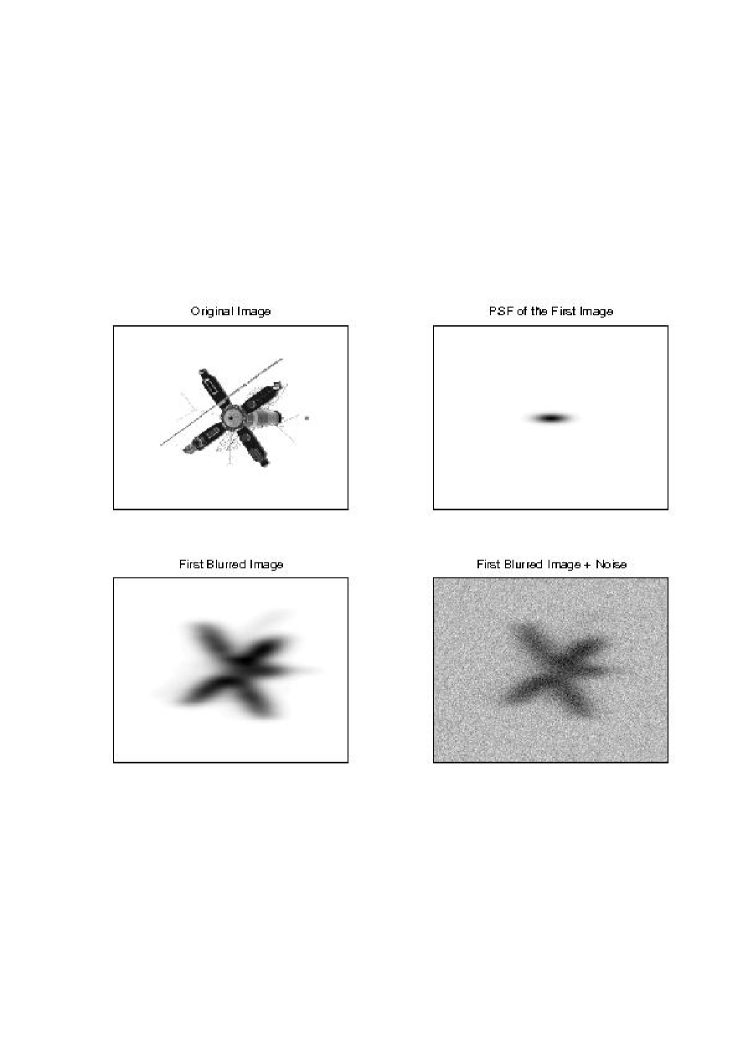
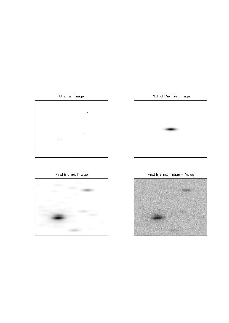
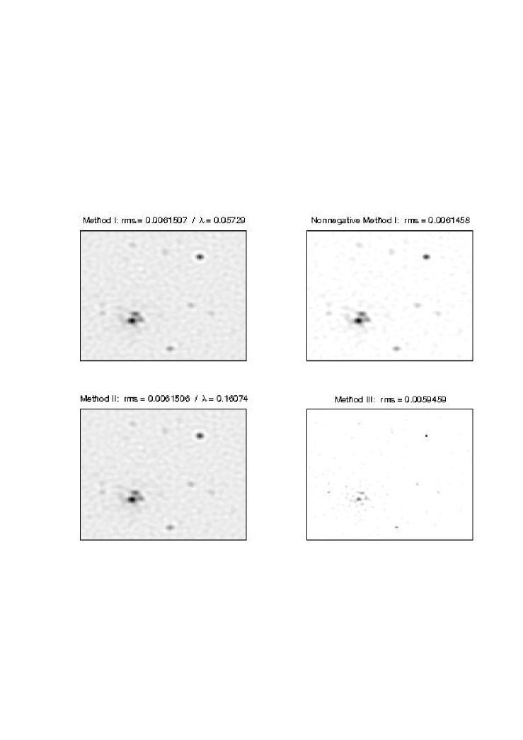
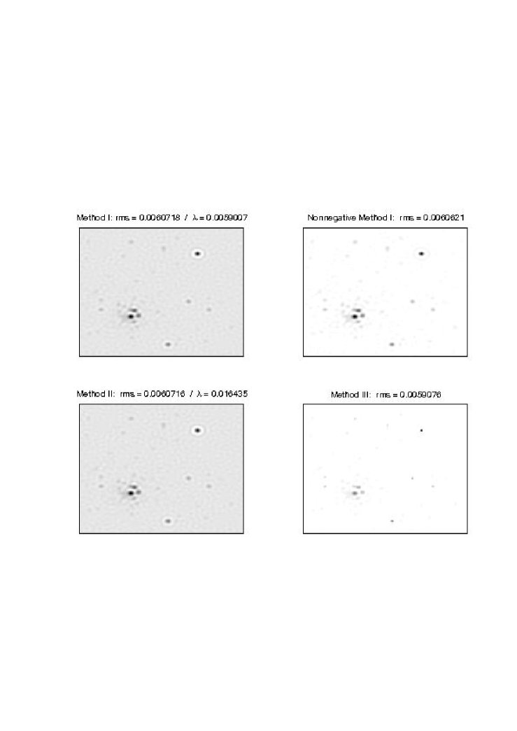
Figures 1-6 compare the deblurring of an extended object with a sharp outline and a set of point-like objects. We have chosen these particular examples because their restoration is a difficult problem. Eight images are available for each object. In each case the PSF is a bidimensional Gaussian with dispersion along the major axis set to twelve pixels, and to four pixels along the minor axis. Their inclinations take equispaced values in the range $0^{\circ}-160^{\circ}$. Gaussian white noise is added with two different levels of noise by setting the standard deviations to $1\%$ and $10\%$, respectively, of the maximum value of the blurred images. Three deblurring methods have been used: (I) single-image Tikhonov based on the functional (12) and the ${\rm GCV_{\alpha}^{(\boldsymbol{\varsigma})}}$ function (3.1) ($\alpha=1.4$); (II) Tikhonov based on the functional (5) and ${\rm GCV_{\alpha}^{(\boldsymbol{g})}}$ function (26) ($\alpha=1.4$); (III) a classic iterative Projected Landweber Method applied to the single-image images for the iterative methods obtained as explained in Vio et al. (2004), that can be used to enforce nonnegativity of the solution (a maximum number of $2000$ iterations has been adopted, that is sufficient to provide results that do not show further appreciable visual changes).

There is no need to test the ${\rm GCV}$ functional (28) because in our case it is identical to (26). The reason is that the shape of all the selected PSFs is the same, they only differ in their orientation, and since orientation information is lost through the trace, the denominator ${\cal D}_{j}$ does not depend on the image index $j$. That is, all the images share the same effective degrees of freedom.

Since the Tikhonov technique does not enforce the nonnegativity constraint, the deblurred images obtained with the single-image approach are also shown with their negative values set to zero. Finally, for each of the experiments, the true “optimal” value (in the sense of the minimization of the rms of the true residuals) for the regularization parameter provided by the ${\rm GCV}$ function (3.1) has been determined, with an accuracy of two significant digits, by a simple grid search. In all cases, the “true” and the estimated regularization parameter have been almost identical. In particular, the relative difference between the rms of the true residuals of the corresponding solutions was always less than $0.3\%$.

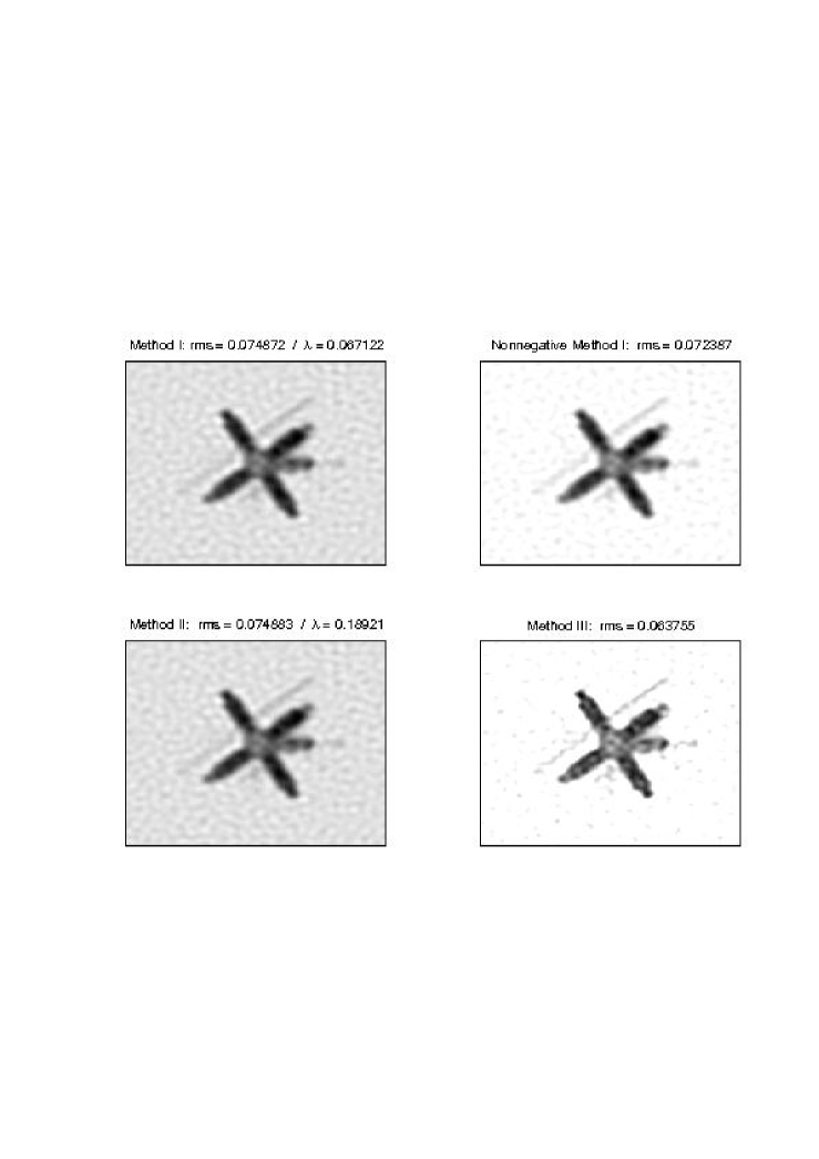
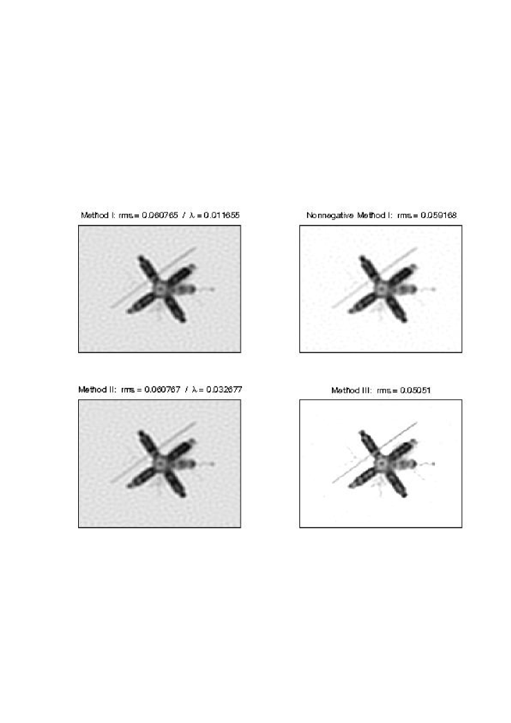
As shown by the figures, the multiple and single-image approaches lead to very similar, if not identical, residual rms values.

As expected, Projected Landweber provides the best results in terms of visual appearance and residual rms. In fact, as is well known, the nonnegativity constraint limits the ringing effect around the sharp structures in the image. However, in these experiments the difference seems important only for point-like objects. In any case, these results are obtained at a very high computational cost (each iteration requires the computation of two two-dimensional DFTs).

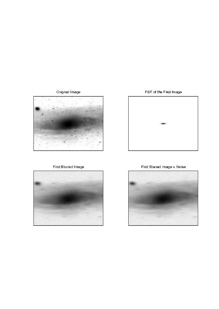
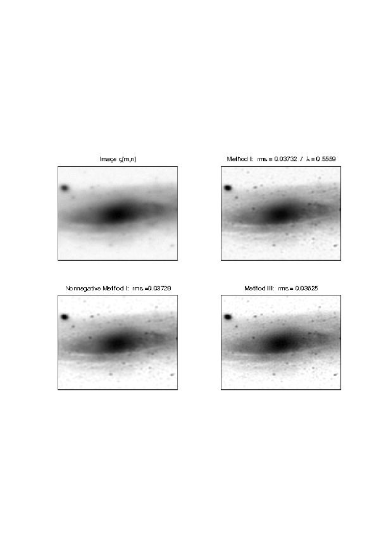
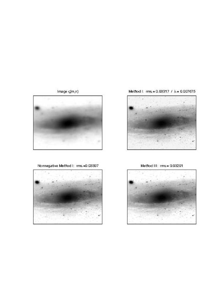
Apart from the nonnegativity constraint, the worst performance of the Tikhonov method is due to the functional $\boldsymbol{L}$ that tends to smooth out structures with sharp features. This characteristic makes Tikhonov more suited for the restoration of images of diffuse objects. In fact, Figs. 7-9 show that for diffuse objects, single-image Tikhonov provides competitive restoration quality (see also Bertero & Boccacci 1998). Because of the presence of features close to the borders of the images, calculations for the image $\varsigma(m,n)$ and the deblurring operation have been implemented with the windowing procedure as explained in Vio et al. (2004). This has required the removal of a border $50$ pixels thick from the image and has only been done with the single-image Tikhonov approach because, given the necessity of windowing each single image, it would be tortuous to implement the other version of the algorithm.

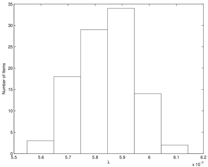
In order to test the stability of the $\lambda$ estimates, for each experiment $100$ realizations of the corresponding noise process are generated and added to the image. In general, the estimates of this parameter appear quite stable; as measured by the rms of the estimated values divided by their median, they fall in the range $1\%-2\%$. Fig. 10 shows the histogram of the values of $\lambda$ obtained with the single-image Tikhonov approach in the experiments with the worst relative variation.

5 Concluding remarks

We have considered the estimation of the regularization parameter for the simultaneous Tikhonov deblurring of multiple noisy images using three types of ${\rm GCV}$ functions based on different data transformations. The first approach reduces the multiple-image problem to single-image deblurring that allows the use of the classical ${\rm GCV}$, but we use a corrected ${\rm GCV}$ that reduces its tendency to undersmooth the final solution. A second approach is perhaps the most natural as it is a straightforward extension of a classical single-image approach. It aims to achieve a balance between the smoothness of the unknown image and its average goodness of fit to the observed images. The regularization parameter is estimated through a multiple-image extension of the traditional ${\rm GCV}$ function. The third approach is based on a higher dimensional single image defined by concatenating all the images into a single vector and then using the classical ${\rm GCV}$.

Our numerical experiments indicate that the three approaches provide very similar results, with the lower-dimensional single image providing the practical advantage that no new software is required and the same image can be used with other deblurring algorithms.

We have assumed that the noise in all the images is independent Gaussian and of constant variance. Combinations of the methods we propose can be used when some of these assumptions are not met. For example, if there are $k$ groups of images with different variances, a weighted Tikhonov regularization method can be applied to a multiple-image deblurring of $k$ single images. In additon, the multiple-image approach can be used if the noise in the original image is correlated but the covariance matrix is known up to a constant (e.g., Gu 2002).

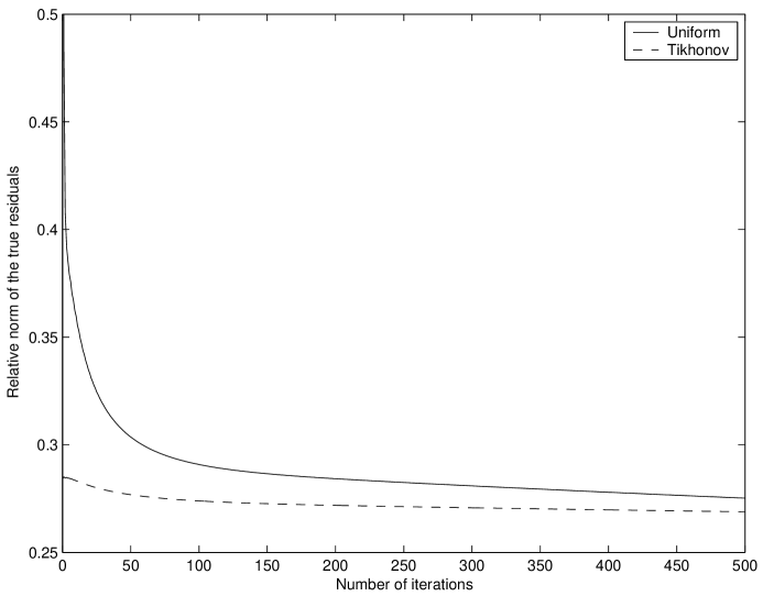
The extreme computational efficiency, coupled with the stability and reliabilty of the estimated regularization parameters, make Tikhonov’s method competitive with the more flexible, but much slower, iterative algorithms. In fact, and especially for very large images, even in situations where these algorithms are expected to provide better results (e.g., when the nonnegativity constraint can be exploited), the Tikhonov approach is still a valuable resource (see also Bertero & Boccacci 2000). For example, it can be used to obtain initial solutions for iterative algorithms that may speed up the convergence. Figure 11 shows the residual rms as a function of iteration number for the Projected Landweber algorithm started at a Tikhonov solution and at the uniform image traditionally used. The figure shows that the saving in computation time can be considerable (here it is more than a factor of $10$).

Figure 1: Original image, blurred version and blurred + noise version of the first image in the set (see text) and corresponding PSF. The images are $256\times 256$ pixels, and the standard deviation of the noise is $10\%$ of the maximum value of the blurred image.

Figure 2: Deblurring of the image in Fig. 1 with the methods decribed in the text: (I) single-image Tikhonov (12) and ${\rm GCV^{(\boldsymbol{\varsigma})}_{\alpha}}$  (3.1); its version with the negative elements zeroed; (II) Tikhonov (5) and ${\rm GCV^{(\boldsymbol{g})}_{\alpha}}$ (26); (III) a classic iterative Projected Landweber Method (convergence after $61$ iterations). Tikhonov has been used with $\boldsymbol{L}=\boldsymbol{I}$ and $\alpha=1.4$.

Figure 3: The same as Fig. 2 but obtained from an image contaminated with noise whose standard deviation is $1\%$ of the maximum value of the blurred image. For the Projected Landweber algorithm $2000$ iterations have been carried out.

Figure 4: Original image, blurred version and blurred + noise version of the first image in the set (see text) and corresponding PSF. The images are $256\times 256$ pixels, and the standard deviation of the noise is $10\%$ of the maximum value of the blurred image.

Figure 5: Deblurring of the image in Fig. 4 with the methods described in the text: (I) single-image Tikhonov (12) and ${\rm GCV^{(\boldsymbol{\varsigma})}_{\alpha}}$  (3.1); its version with the negative elements zeroed; (II) Tikhonov (5) and ${\rm GCV^{(\boldsymbol{g})}_{\alpha}}$ (26); (III) a classic iterative Projected Landweber Method ($2000$ iterations). Tikhonov has been used with $\boldsymbol{L}=\boldsymbol{I}$ and $\alpha=1.4$.

Figure 6: The same as Fig. 5 but obtained from an image contaminated with noise whose standard deviation is $1\%$ of the maximum value of the blurred image.

Figure 7: Original image, blurred version and blurred + noise version of the first image in the set (see text) and corresponding PSF. The original images was $600\times 600$ pixels, but only the central $500\times 500$ pixels are displayed (see text). The standard deviation of the noise is $10\%$ of the standard deviation of the blurred image.

Figure 8: Image $\varsigma(m,n)$ for the image shown in Fig. 4, single-image Tikhonov deblurring ($\boldsymbol{L}=$ discrete Laplacian), its version with the negative elements zeroed, and the iterative Projected Landweber deblurring (convergence after $24$ iterations).

Figure 9: The same as Fig. 8 but obtained from an image contaminated with noise whose standard deviation is $1\%$ of the standard deviation of the blurred image. Tikhonov has been used with $\boldsymbol{L}=\boldsymbol{I}$. For the Projected Landweber algorithm $2000$ iterations have been carried out.

Figure 10: Histogram of the values of the estimated parameter $\lambda$ for the $100$ experiments based on Fig. 6.

Figure 11: Convergence rates for the Projected Landweber algorithm in the numerical experiment corresponding to Fig. 3. Two starting guesses are used: the uniform image typical of the classic implementation of the algorithm, and the nonnegative single-image Tikhonov shown in Fig. 3.

Appendix A Derivation of Eq.(19)

Let $\boldsymbol{e}_{i}$ be the vector with 1 in the $i$th entry and zero everwhere else, and $\boldsymbol{\tilde{f}}_{k,-i}$ the estimate of $\boldsymbol{f}$ that does not use the $i$th entry of $\boldsymbol{g}_{k}$. We can write

$$g_{k,i}=\boldsymbol{e}_{i}^{T}\boldsymbol{g}_{k},\qquad\widehat{g}_{k,-i}=\boldsymbol{e}_{i}^{T}\boldsymbol{A}_{k}\boldsymbol{\tilde{f}}_{k,-i}.$$

Let $\boldsymbol{P}_{i}$ be the projection that deletes the $i$th entry:

$$\boldsymbol{g}_{k,-i}=\boldsymbol{P}_{i}\boldsymbol{g}_{k}$$

so that $\boldsymbol{P}_{i}^{T}\boldsymbol{P}_{i}=\boldsymbol{I}-\boldsymbol{e}_{i}\boldsymbol{e}_{i}^{T}$. Let

$$\boldsymbol{a}_{ki}=\boldsymbol{A}_{k}^{T}\boldsymbol{e}_{i},\qquad\boldsymbol{H}_{k}=\boldsymbol{A}_{k}(\,\boldsymbol{A}+\lambda\boldsymbol{I}\,)^{-1}\boldsymbol{A}_{k}^{T},$$

then, by definition,

$$\boldsymbol{\tilde{f}}_{k,-i} =\left(\,\sum_{i\neq k}\boldsymbol{A}_{i}^{T}\boldsymbol{A}_{i}+\boldsymbol{A}_{k}^{T}\boldsymbol{P}_{i}^{T}\boldsymbol{P}_{i}\boldsymbol{A}_{k}+\lambda\boldsymbol{I}\,\right)^{-1}$$

$$\times\left(\,\sum_{i\neq k}\boldsymbol{A}_{i}^{T}\boldsymbol{g}_{i}+\boldsymbol{A}_{k}^{T}\boldsymbol{P}_{i}^{T}\boldsymbol{P}_{i}\boldsymbol{g}_{k}\,\right)$$

$$= \left(\,\boldsymbol{A}+\lambda\boldsymbol{I}-\boldsymbol{A}_{k}^{T}\boldsymbol{e}_{i}\boldsymbol{e}_{i}^{T}\boldsymbol{A}_{k}\,\right)^{-1}\left(\,\boldsymbol{\vartheta}-\boldsymbol{A}_{k}^{T}\boldsymbol{e}_{i}\boldsymbol{e}_{i}^{T}\boldsymbol{g}_{k}\,\right)$$

$$= \left[\,(\,\boldsymbol{A}+\lambda\boldsymbol{I}\,)^{-1}+\frac{(\,\boldsymbol{A}+\lambda\boldsymbol{I}\,)^{-1}\boldsymbol{a}_{ki}\boldsymbol{a}_{ki}^{T}(\,\boldsymbol{A}+\lambda\boldsymbol{I}\,)^{-1}}{1-\boldsymbol{a}_{ki}^{T}(\,\boldsymbol{A}+\lambda\boldsymbol{I}\,)^{-1}\boldsymbol{a}_{ki}}\,\right]$$

$$\times\left(\,\boldsymbol{\vartheta}-\boldsymbol{A}_{k}^{T}\boldsymbol{e}_{i}\boldsymbol{e}_{i}^{T}\boldsymbol{g}_{k}\,\right).$$

It follows that

$$\boldsymbol{A}_{k}\boldsymbol{\tilde{f}}_{k,-i}=\boldsymbol{A}_{k}\boldsymbol{\tilde{f}}-\boldsymbol{H}_{k}\boldsymbol{e}_{i}\boldsymbol{e}_{i}^{T}\boldsymbol{g}_{k}$$

$$+\frac{\boldsymbol{H}_{k}\boldsymbol{e}_{i}\boldsymbol{a}_{ki}^{T}(\,\boldsymbol{A}+\lambda\boldsymbol{I}\,)^{-1}\boldsymbol{\vartheta}-\boldsymbol{H}_{k}\boldsymbol{e}_{i}\boldsymbol{e}_{i}^{T}\boldsymbol{H}_{k}\boldsymbol{e}_{i}\boldsymbol{e}_{i}^{T}\boldsymbol{g}_{k}}{1-(\boldsymbol{H}_{k})_{ii}}$$

$$\boldsymbol{e}_{i}^{T}\boldsymbol{A}_{k}\boldsymbol{\tilde{f}}_{k,-i} -{\tilde{g}}_{ki}=\frac{(\boldsymbol{H}_{k})_{ii}}{1-(\boldsymbol{H}_{k})_{ii}}$$

$$\times\left(\boldsymbol{a}_{ki}^{T}(\,\boldsymbol{A}+\lambda\boldsymbol{I}\,)^{-1}\boldsymbol{\vartheta}-\boldsymbol{e}_{i}^{T}\boldsymbol{g}_{k}\,\right)$$

$$=\frac{(\boldsymbol{H}_{k})_{ii}}{1-(\boldsymbol{H}_{k})_{ii}}\,\left(\,\boldsymbol{e}_{i}^{T}\boldsymbol{A}_{k}\boldsymbol{\widehat{f}}-g_{ki}\,\right)$$

$$=\frac{(\boldsymbol{H}_{k})_{ii}}{1-(\boldsymbol{H}_{k})_{ii}}\,\left(\,{\tilde{g}}_{ki}-g_{ki}\,\right)$$

$${\tilde{g}}_{k,-i}-g_{ki}={\tilde{g}}_{ki}-g_{ki}+\frac{(\boldsymbol{H}_{k})_{ii}}{1-(\boldsymbol{H}_{k})_{ii}}\,\left(\,{\tilde{g}}_{ki}-g_{ki}\,\right)$$

$${\tilde{g}}_{k,-i}-g_{ki}=\frac{1}{1-(\boldsymbol{H}_{k})_{ii}}\,\left(\,{\tilde{g}}_{ki}-g_{ki}\,\right).$$

References

• Angel et al. (1998) Angel, J.R.P., Hill, J.M., Strittmatter, P.A., Salinari, P., & Weigelt, G., 1998, in: Astronomical Interferometry, eds., R.D. Reasenberg, Proc. SPIE, 3352, 881
• Bertero & Boccacci (1998) Bertero, M., & Boccacci, P. 1998, Introduction to Inverse Problems in Imaging (IOP Publishing, Bristol)
• Bertero & Boccacci (2000) Bertero, M., & Boccacci, P. 2000, A&A, 147, 323
• Gu (2002) Gu, C. 2002, Smoothing Spline ANOVA Models (Springer-Verlag, New York)
• Cummins et al. (2001) Cummins, D. J., Filloon, T. G., & Nychka, D. 2001, Journal of the American Statistical Association, 96, 233
• Kim & Gu (2004) Kim, Y.J., & Gu, C. 2004, Journal of the Royal Statistical Society (B), 66, 337
• Lehmann & Casella (1998) Lehmann, E. L. & Casella, G. 1998, Theory of Point Estimation (Springer-Verlag, New York)
• Nychka et. al. (1998) Nychka, D., Haaland, P.D., O’Connell, M.A., & Ellner, S. 1998, Case Studies in Environmental Statistics, Nychka et. al., eds. (Springer-Verlag, New York)
• Vio et al. (2003) Vio, R., Nagy, J., Tenorio, L., et al. 2003, A&A, 401, 389
• Vio et al. (2004) Vio, R., Nagy, J., Tenorio, L., & Wamsteker 2004, A&A, 416, 403
• Wahba (1985) Wahba, G. 1985, Ann. Stat., 13, 1378
• Wahba (1990) Wahba, G. 1990, Spline Models for Observational Data (SIAM, Philadelphia)