A View through Faraday’s Fog 2:
Parsec Scale Rotation Measures in 40 AGN

Abstract

Results from a survey of the parsec scale Faraday rotation measure properties for 40 quasars, radio galaxies and BL Lac objects are presented. Core rotation measures for quasars vary from approximately 500 to several thousand rad m^-2 . Quasar jets have rotation measures which are typically 500 rad m^-2 or less. The cores and jets of the BL Lac objects have rotation measures similar to those found in quasar jets. The jets of radio galaxies exhibit a range of rotation measures from a few hundred rad m^-2 to almost 10,000 rad m^-2 for the jet of M87. Radio galaxy cores are generally depolarized, and only one of four radio galaxies (3C 120) has a detectable rotation measure in the core. Several potential identities for the foreground Faraday screen are considered and we believe the most promising candidate for all the AGN types considered is a screen in close proximity to the jet. This constrains the path length to approximately 10 parsecs, and magnetic field strengths of approximately 1 $\mu$Gauss can account for the observed rotation measures. For 27 out of 34 quasars and BL Lacs their optically thick cores have good agreement to a $\lambda^{2}$ law. This requires the different $\tau=1$ surfaces to have the same intrinsic polarization angle independent of frequency and distance from the black hole.

1 Introduction

The first rotation measure (RM) towards an extragalactic radio source was published by Cooper & Price (1962). They discussed the potential for such measurements as a probe of the galactic Faraday screen. Wardle (1977) analyzed radio polarization monitoring observations of compact extragalactic sources for signs of Faraday rotation. Wardle suggested that the combined Faraday rotation from our galaxy and the host object were relatively small. Observations on arcsecond scales of 555 steep spectrum sources by Simard-Normandin, Kronberg, & Button (1981), and of flat spectrum sources by Rudnick & Jones (1983) and Rusk (1988) all confirmed this result. An expectation was established using these observations that the unresolved parsec scale cores of AGN would similarly show negligible Faraday rotation. It was not until simultaneous, multi-frequency polarimetry became available with the Very Long Baseline Array (VLBA) that these expectations were proven false. Extreme parsec scale rest frame rotation measures were first reported for OQ 172 (Udomprasert et al., 1997, 40000 rad m^-2 ) and 3C 138 (Cotton et al., 1997, 5300 rad m^-2 ). Such RMs show that interpretations of polarization observations on parsec scales in AGN requires simultaneous determination of the rotation measure. Without knowledge of the rotation measure in a source the orientations of polarization vectors in the relativistic jets of AGN is uncertain. For example, a rotation measure of 250 rad m^-2 will change the intrinsic polarization angle of a source by 25^∘ at 8 GHz. The existence of RMs in quasar cores of 1000 rad m^-2 or more (Taylor, 1998, 2000) and time variability of RMs in quasar cores (Zavala & Taylor, 2001) shows how essential knowledge of the rotation measure is for the correct interpretation of the observed polarization.

Michael Faraday first observed what we now refer to as Faraday rotation when he passed polarized light through glass in the presence of a magnetic field (Faraday, 1933). He correctly surmised that this observation hinted at the connection between electric and magnetic fields and light. Light subject to Faraday rotation will have its intrinsic polarization angle $\chi_{0}$ rotated to an observed angle $\chi$ by

$$\chi=\chi_{0}+\rm{RM}{\lambda}^{2}$$ (1)

where $\lambda$ is the observed wavelength. The linear relationship to $\lambda^{2}$ is the characteristic signature of Faraday rotation. The slope of the line is known as the Rotation Measure (RM) and depends linearly on the electron density $\rm{n_{e}}$, the net line of sight magnetic field $\rm{B_{\parallel}}$, and path length $\rm{dl}$ through the plasma. Using units of cm^-3, mG and parsecs the rotation measure is given by:

$$\rm{RM=812\int{n_{e}B_{\parallel}\,dl}\quad rad\ m^{-2}}.$$ (2)

A suitably designed experiment can resolve the n$\pi$ ambiguity inherent in polarization vector orientations. By obtaining observations with sufficient long and short spacings in $\lambda^{2}$ this ambiguity can be resolved, and the correct RM determined.

This paper completes the presentation of a rotation measure survey of 40 AGN suggested in Taylor (2000). The first half of the observations appeared in Zavala & Taylor (2003). We present our observations and data reduction procedures in §2. Results for individual sources are shown in §3. In §4 we consider the rotation measure properties of the sample as a whole, including a few additional sources in the literature. Conclusions appear in §5.

2 Observations and Data Reduction

The observations, performed on 2001 June 20 (2001.47), were carried out at seven widely separated frequencies between 8.1 and 15.2 GHz using the 10 element VLBA. This 24 hour observation targeted the sources listed in Table 1. Due to an electrical short in the elevation system the Ft. Davis antenna was lost for the first 7.5 hours of the 24 hour run. Prior to self-calibration all processing was performed in the Astronomical Image Processing System (AIPS; van Moorsel, Kemball, & Greisen, 1996). AIPS procedures described in Ulvestad, Greisen & Mioduszewski (2001) were employed and are indicated by eight letter capitalized words (e.g. VLBACPOL). Data collected at elevations less than 10^∘ were flagged. Amplitude calibration was performed with the task APCAL. An opacity correction was employed at all frequencies as several antennas (Pie Town, Ft. Davis, Kitt Peak, and Hancock) reported rain during the observation. Plots of T_sys versus airmass also indicated a variable opacity at North Liberty. The procedure VLBAPANG corrected the observations for varying parallactic angles of the alt-azimuth mounted VLBA antennas. VLBAMPCL was used on two minutes of data from 3C 279 to remove errors due to clock and correlator model inaccuracies. A global fringe fit was run on all the data to remove the remaining delay and rate errors with the procedure VLBAFRNG. VLBAFRNG uses the AIPS task FRING, an implementation of the Schwab$-$Cotton algorithm (Schwab & Cotton, 1983). The delay offset between the right and left circularly polarized data was removed using the procedure VLBACPOL (Cotton, 1993). A bandpass correction table was made with BPASS using 1741$-$038 as a bandpass calibrator. The data were then averaged in frequency across the individual intermediate frequencies (IFs).

Self-calibration was done using DIFMAP (Shepherd, 1997; Shepherd, Pearson & Taylor, 1994) and AIPS in combination. Considerable radio frequency interference was present at 12 GHz on almost all baselines for 3C 279 and 3C 446, and was edited out. This resulted in the loss of 49% of the visibilities for 3C 279 and 23% for 3C 446 at 12 GHz. As the gain curves of the antennas used in the amplitude calibration are poorly known at 12 GHz we compared the VLBA flux at 12 GHz with that from the VLA Polarization Monitoring web page (Taylor & Myers, 2000) and data from the University of Michigan Radio Astronomy Observatory (UMRAO; H. Aller, 2003, private communication). This comparison suggested a reduction of approximately 10% in the gain solution was required at 12 GHz, and this was applied with the task SNCOR. Table 1 lists the number of scans on each source, as well as the RMS and peak flux in the 15 GHz I map that this calibration produced. Scans were three and one half minutes long. If all ten antennas are present in 7 scans the expected thermal noise at 15 GHz is approximately 0.5 mJy beam^-1.

Polarization leakage of the antennas (D-terms) were determined using the AIPS task LPCAL (Leppänen, Zensus, & Diamond, 1995). We chose 0552+398 as the D-term calibrator as it had a wide parallactic angle coverage, and a simple and nearly unresolved polarization structure. Plots of the real versus imaginary crosshand polarization data indicated that a satisfactory D-term solution was obtained. This was also verified in plots of the real and imaginary crosshand data versus (u,v) parallactic angle. After applying the D-term solution no variation was seen as a function of (u,v) parallactic angle.

Absolute electric vector position angle (EVPA) calibration was determined by using the EVPA of 3C 279 listed in the VLA Polarization Monitoring Program. We used the integrated Q and U fluxes from the VLBA data to derive a position angle, which we compared to that listed on the polarization monitoring web page. This calibration scheme rests on the assumption that most of the polarized flux observed by the VLA is seen with the VLBA. To verify this the polarized flux observed by UMRAO, the VLA and the VLBA are listed in Table 2 for 8 and 15 GHz, with their respective observation dates. The good agreement between these values for telescopes with very different resolutions makes us confident in our absolute EVPA calibration. The position angles for 3C 279 were observed with the VLA in B array on 2001 Jun 24. These position angles were in good agreement with nearly contemporaneous observations from the UMRAO data for 3C 279. The EVPA calibration at 8 GHz was directly obtained from the polarization calibration website. Polarization monitoring observations at 8 and 22 GHz were interpolated to produce position angles at 12 and 15 GHz, assuming the EVPA’s obeyed a $\lambda^{2}$ Faraday rotation law. Fig. 1 shows the final calibrated VLBA EVPA’s with the VLA EVPA’s from the polarization monitoring webpage.

The uncertainty in the EVPA calibration using the RM fit in Fig. 1 is approximately $\pm$1 degree. To this uncertainty we add in quadrature the uncertainty derived from the individual Stokes Q and U maps. There will be some additional uncertainty from the lack of simultaneous VLA polarization observations which is difficult to quantify. Data obtained with UMRAO and the VLA to establish the EVPA calibration were taken within 1-5 days of the VLBA observation. If the lack of simultaneous observations by the VLA and/or UMRAO were significant we would expect all the fits to a $\lambda^{2}$ law to require a systematic increase in their error budget. Although some sources do not show good agreement to a $\lambda^{2}$ law many do, and thus we conclude that the errors have been properly accounted for.

To perform the rotation measure analysis data cubes in $\lambda^{2}$ were constructed. The upper and lower pairs of 12 GHz IFs and all four 15 GHz IFs were averaged to improve the signal to noise ratio and to obtain long and short spacings in $\lambda^{2}$. Final frequencies used for the RM analysis are shown in Table 3. This provides adequate short and long spacings in $\lambda^{2}$ to properly recover RMs between $\pm$ 30000 rad m^-2. The 12 and 15 GHz images used to produce the polarization angle maps were tapered to approximate the 8 GHz resolution, and a restoring beam matched to the 8 GHz beam was used. All images are naturally weighted.

3 Results

Maps showing the rotation measure, RM corrected electric vectors and spectral index between 8.5 and 12.1 GHz are presented. If the fits to a $\lambda^{2}$ law do not appear satisfactory a reduced $\chi^{2}$ test was performed. If the reduced $\chi^{2}$ indicates that a $\lambda^{2}$ law is ruled out at a 3$\sigma$ level or higher we remove the source from consideration when examining the RM properties of the sample as a whole (§4).

3.1 B0202+149

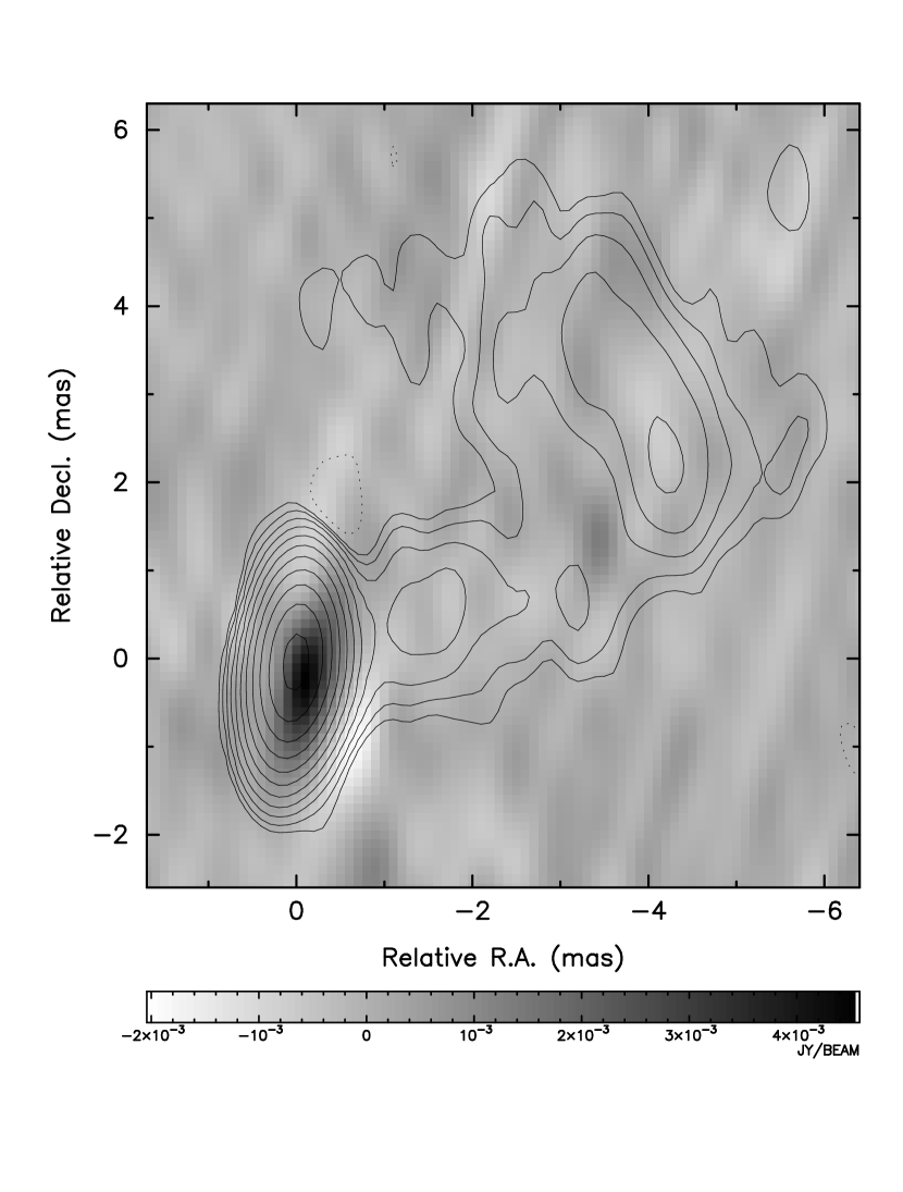
Figure 2: Full resolution 15 GHz Stokes U flux in greyscale overlaid on Stokes I contours at 15 GHz for B0202+149. Contours start at 1.2 mJy beam^-1 and increase by factors of two.

This object was depolarized at 12 and 8 GHz, and thus no rotation measure image is provided. The object is classified as a blazar at a redshift of 0.405 (Perlman et al., 1998). Observations of superluminal motion (Pyatunina et al., 2000), a brightness temperature in excess of of 10¹² K (Moellenbrock et al., 1996), and the high probability of detection with EGRET (Mattox et al., 1997) all agree with a blazar identification for this source. This is surprising as unlike other blazars such as 3C 279 and BL Lac (Zavala & Taylor, 2003, and references therein) there is no detectable rotation measure in 0202+149. This is the case for another EGRET detected blazar, 0420$-$014 (Zavala & Taylor, 2003), whose depolarization seems to be explained by the superposition of components of differing position angles. For 0202+149 this may be the case. The source is only detected in polarization in Stokes U at 15 GHz and a full resolution image (Fig. 2) shows two components of Stokes U of opposite sign and but different magnitude. The negative U component is only weakly detected. Tapering and restoring with a beam matched to the 8 GHz resolution nearly eliminates the polarized components of 0202+149 at 15 GHz.

3.2 B0336$-$019

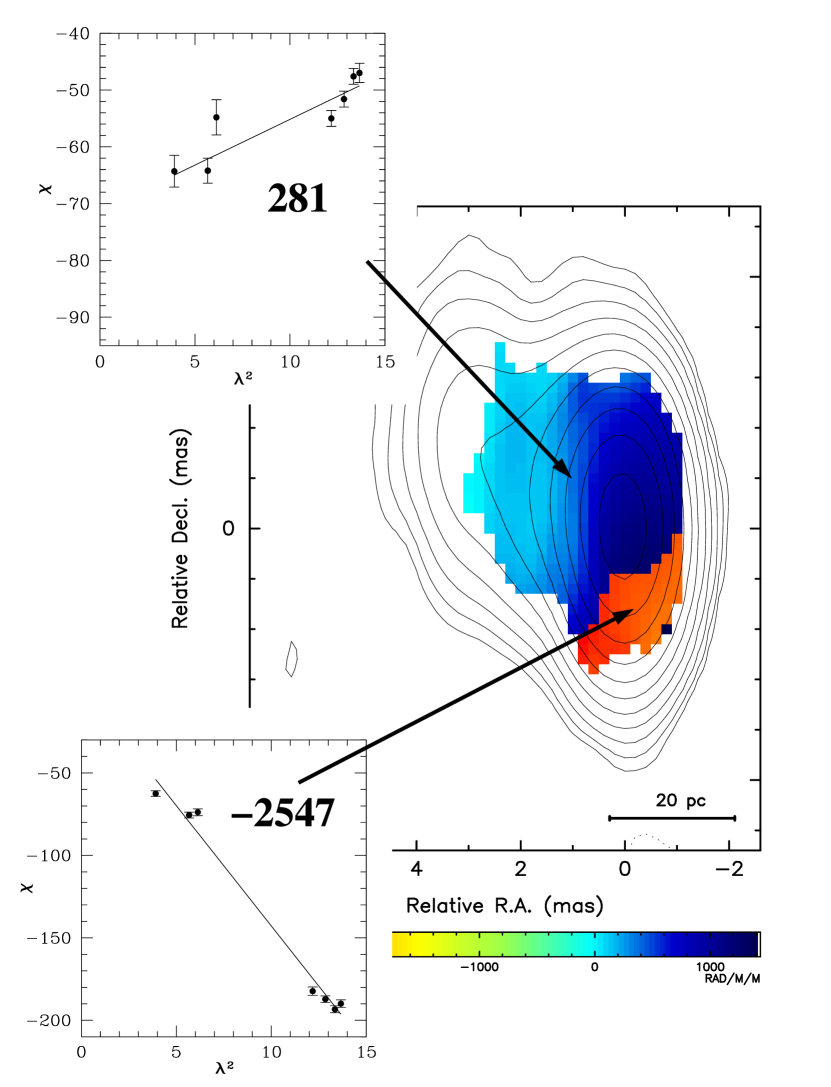
Figure 3: (a) Rotation measure image (color) for 0336$-$019 overlaid on Stokes I contours at 15 GHz. The inset is a plot of EVPA $\chi$ (deg) versus $\lambda^{2}$ (cm²). (b) Electric vectors (1 mas = 67 mJy beam^-1 polarized flux density) corrected for Faraday Rotation overlaid on Stokes I contours. Contours start at 1.5 mJy beam^-1 and increase by factors of two.

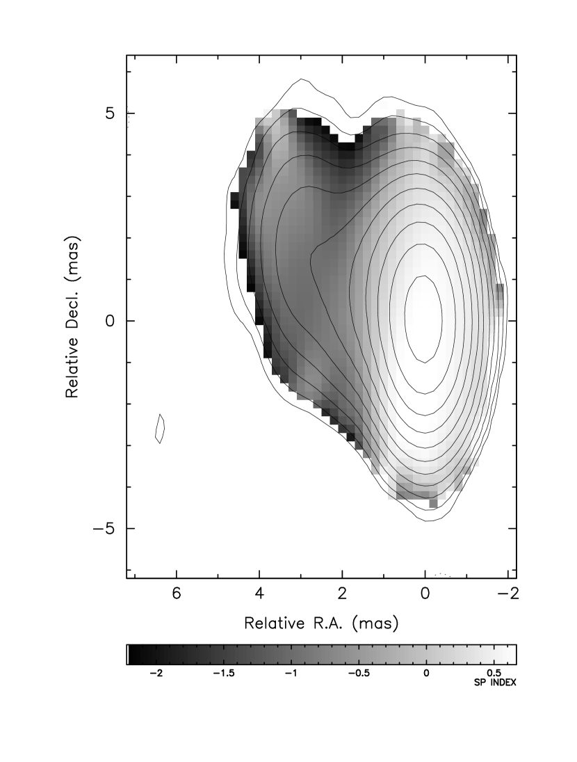
Figure 4: Spectral index $\alpha_{12.1}^{8.1}$ plot for 0336$-$019 overlaid on Stokes I contours at 15 GHz. Contours start at 1.5 mJy beam^-1 and increase by factors of two.

This source has an RM of $-$2547 $\pm$ 33 rad m^-2  which decreases to 281 $\pm$ 37 rad m^-2 (Fig. 3a). A sharp border between the negative slope to the RM in the core and the positive slope in the jet coincides with a change in the intrinsic electric vector direction as shown in Fig. 3b. This change in the slope of the RM and electric vector orientation occurs as the spectral index changes from positive to negative (Fig. 4).

The quality of the fits to a $\lambda^{2}$ law for this quasar appear suspect (Fig. 3a). The reduced $\chi^{2}$ of the fits are 7.7 or larger. With 5 degrees of freedom this implies that a $\lambda^{2}$ law can be ruled out with a confidence of more than 3$\sigma$.

3.3 B0355+508

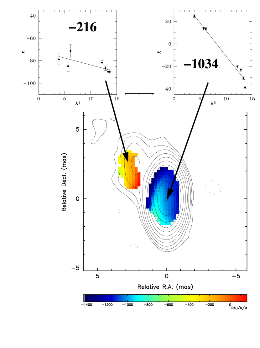
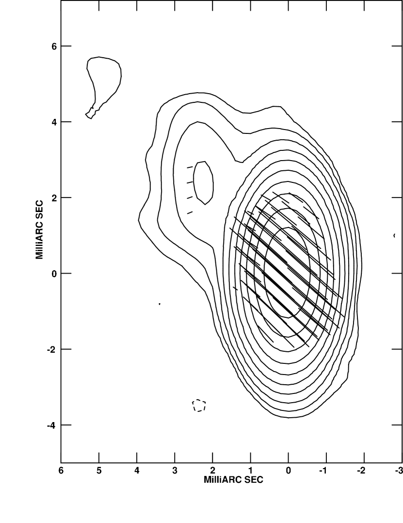
Figure 5: (a) Rotation measure image (color) for 0355+508 overlaid on Stokes I contours at 15 GHz. The inset is a plot of EVPA $\chi$ (deg) versus $\lambda^{2}$ (cm²). (b) Electric vectors (1 mas = 67 mJy beam^-1 polarized flux density) corrected for Faraday Rotation overlaid on Stokes I contours. Contours start at 6.9 mJy beam^-1 and increase by factors of two.

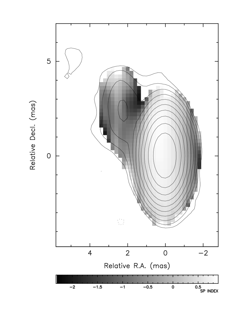
Figure 6: Spectral index $\alpha_{12.1}^{8.1}$ plot for 0355+508 overlaid on Stokes I contours at 15 GHz. Contours start at 6.9 mJy beam^-1 and increase by factors of two.

Also known as NRAO 150, this source has no optical counterpart and thus no redshift available. The RM in the core is $-1034\pm 21$ rad m^-2 and this decreases by approximately a factor of five ($-216\pm 65$ rad m^-2) in the jet component (Fig. 5a). The core and jet have very different electric vector orientations (Fig. 5b), but it should be noted that the signal in the jet component is fairly weak as can be seen in the inset EVPA vs. $\lambda^{2}$ plot in Fig. 5a. As Fig. 6 shows, the core is optically thick, while the jet component is optically thin.

The 8 GHz core EVPA values suggest a non-linear variation of $\chi$ with $\lambda^{2}$. However, the reduced $\chi^{2}$ for the core cannot rule out a Faraday rotation law at a level of $3\sigma$ or higher, and we therefore conclude that the core of 0355+508 adheres to the $\lambda^{2}$ law. The reduced $\chi^{2}$ for the RM fits in the jet can rule out a $\lambda^{2}$ at a level of $3\sigma$ or more, and we conclude that the data for the jet are not consistent with the $\lambda^{2}$ law.

3.4 B0458$-$020

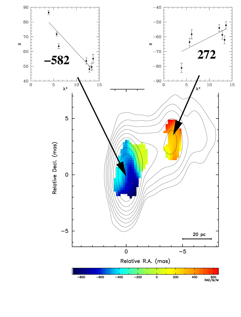
Figure 7: (a) Rotation measure image (color) for 0458$-$020 overlaid on Stokes I contours at 15 GHz. The inset is a plot of EVPA $\chi$ (deg) versus $\lambda^{2}$ (cm²). (b) Electric vectors (1 mas = 25 mJy beam^-1 polarized flux density) corrected for Faraday Rotation overlaid on Stokes I contours. Contours start at 1.4 mJy beam^-1 and increase by factors of two.

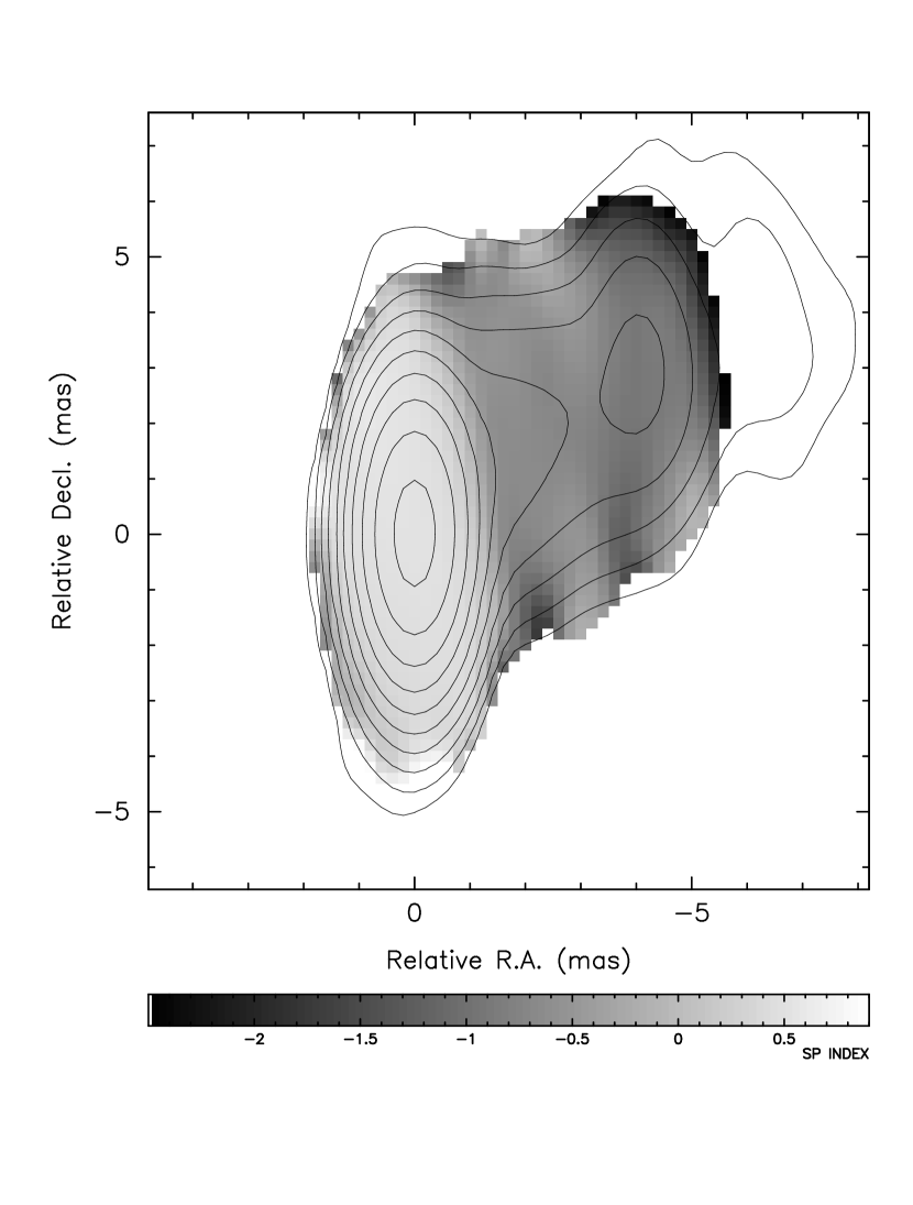
Figure 8: Spectral index $\alpha_{12.1}^{8.1}$ plot for 0458$-$020 overlaid on Stokes I contours at 15 GHz. Contours start at 1.4 mJy beam^-1 and increase by factors of two.

Fig. 7a shows that the fits to a $\lambda^{2}$ law are not very convincing for this source. The RM of $-582\pm 32$ rad m^-2 has a reduced $\chi^{2}$ of 12. The $3\sigma$ confidence level with 5 degrees of freedom is approximately 3.1, and we reject the $\lambda^{2}$ law for the core of 0458$-$020. Similarly, we reject the $\lambda^{2}$ law for the jet as the reduced $\chi^{2}$ is 6. Assuming Faraday rotation does apply to 0458$-$020 we see in Fig. 7b that the jet and core have nearly the same electric vector alignments. 0458$-$020 has an optically thick core and optically thin jet (Fig. 8).

3.5 B0552+398

O’Dea et al. (1990) classify 0552+398 as a gigahertz peaked spectrum (GPS) source. Infrared imaging suggests it is an interacting galaxy in a dense cluster (Hutchings et al., 1999). Wills & Wills (1976) note that the redshift of 0552+398 is uncertain because of a lack of firmly identified spectral lines.

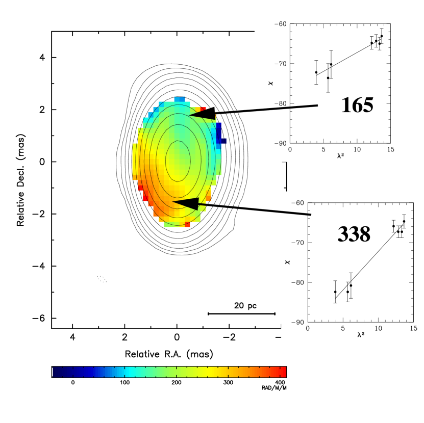
Figure 9: (a) Rotation measure image (color) for 0552+398 overlaid on Stokes I contours at 15 GHz. The inset is a plot of EVPA $\chi$ (deg) versus $\lambda^{2}$ (cm²). (b) Electric vectors (1 mas = 25 mJy beam^-1 polarized flux density) corrected for Faraday Rotation overlaid on Stokes I contours. Contours start at 2.7 mJy beam^-1 and increase by factors of two.

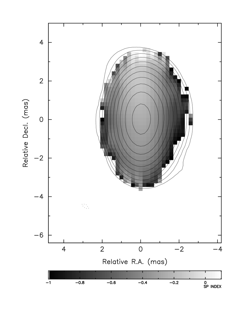
Figure 10: Spectral index $\alpha_{12.1}^{8.1}$ plot for 0552+398 overlaid on Stokes I contours at 15 GHz. Contours start at 2.7 mJy beam^-1 and increase by factors of two.

We are just able to resolve a rotation measure gradient across this source, as shown in Fig. 9a. The RM changes from 338 $\pm$ 39 rad m^-2 to 165 $\pm$ 45 rad m^-2. This gradient is across a projected distance of 20 pc. This distance would incorporate the high RM core and lower RM jet in 3C 273 shown in Zavala & Taylor (2001). The 8$-$15 GHz RM image of 3C 273 in Zavala & Taylor (2001) showed lower RMs than the the higher resolution 15$-$43 GHz RM images. Therefore a much higher RM may be hidden under the coarse spatial resolution of our image. RM corrected electric vectors are aligned East-West (Fig. 9b). The spectral index changes from approximately 0 in the north to $-$0.5 or less in the south (Fig. 10).

3.6 B0605$-$085

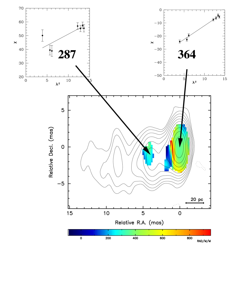
Figure 11: (a) Rotation measure image (color) for 0605$-$085 overlaid on Stokes I contours at 15 GHz. The inset is a plot of EVPA $\chi$ (deg) versus $\lambda^{2}$ (cm²). (b) Electric vectors (1 mas = 25 mJy beam^-1 polarized flux density) corrected for Faraday Rotation overlaid on Stokes I contours. Contours start at 1.5 mJy beam^-1 and increase by factors of two.

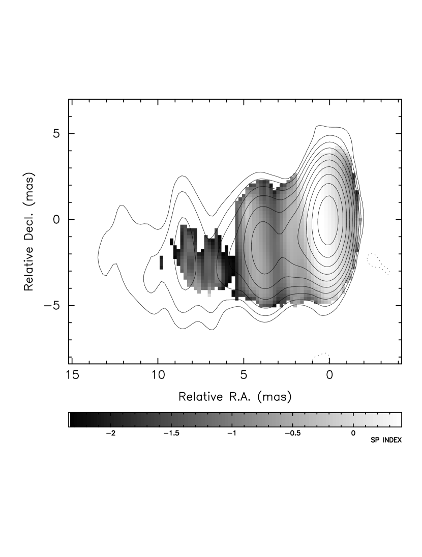
Figure 12: Spectral index $\alpha_{12.1}^{8.1}$ plot for 0605$-$085 overlaid on Stokes I contours at 15 GHz. Contours start at 1.5 mJy beam^-1 and increase by factors of two.

The core and jet component 4 mas east of the core show similar RMs, although there is a lower SNR at the higher frequencies for the jet component (Fig. 11a). The inset plots in Fig. 11a have RMs of 364 $\pm$ 20 rad m^-2 and 287 $\pm$ 57 rad m^-2. About 2 mas SE of the core there seems to be a flattening of the RM slope, and this is coincident with a change in the RM corrected EVPA (Fig. 11b). Fig. 12 shows that this region 2 mas from the core marks the transition to a negative spectral index.

As the SNR for the RM fit in the jet appears rather low we examined the reduced $\chi^{2}$ for both the jet and core RM fits. The core RM fits all have reduced $\chi^{2}$ consistent with a $\lambda^{2}$ law with values less than the 3$\sigma$ level. Even the apparently poor RM fit in the jet has a reduced $\chi^{2}$ of 2.1, and thus consistent with a $\lambda^{2}$ law interpretation.

3.7 B0736+017

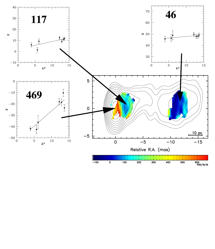
Figure 13: (a) Rotation measure image (color) for 0736+017 overlaid on Stokes I contours at 15 GHz. The inset is a plot of EVPA $\chi$ (deg) versus $\lambda^{2}$ (cm²). (b) Electric vectors (1 mas = 17 mJy beam^-1 polarized flux density) corrected for Faraday Rotation overlaid on Stokes I contours. Contours start at 1.5 mJy beam^-1 and increase by factors of two.

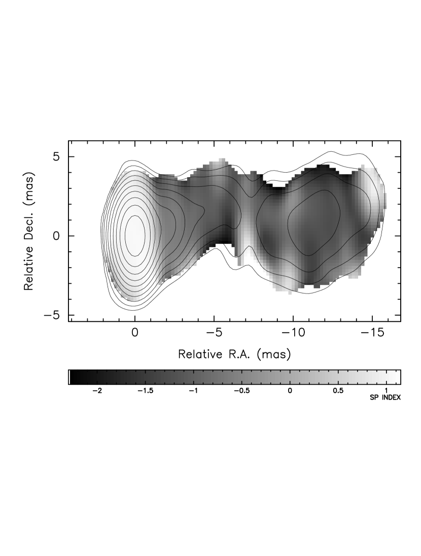
Figure 14: Spectral index $\alpha_{12.1}^{8.1}$ plot for 0736+017 overlaid on Stokes I contours at 15 GHz. Contours start at 1.5 mJy beam^-1 and increase by factors of two.

This quasar has recently been shown to exhibit a dramatic optical flare, and shows evidence for microvariability (Clements, Jenks & Torres, 2003). The weakly polarized core (0.6%) has an RM of $469\pm 40$ rad m^-2 (Fig. 13a), but approximately 50% of the pixels within a beam area centered on the core have a reduced $\chi^{2}$ which rules out a $\lambda^{2}$ law at a level greater than $3\sigma$. We thus reject the optically thick (Fig. 14) core as a region where the Faraday rotation law applies. Beyond a beamwidth ($\approx$1mas west) of the core the reduced $\chi^{2}$ values are consistent with a $\lambda^{2}$ law, and the spectrum changes to optically thin 2-3mas west of the core (Fig. 14).

3.8 B0748+126

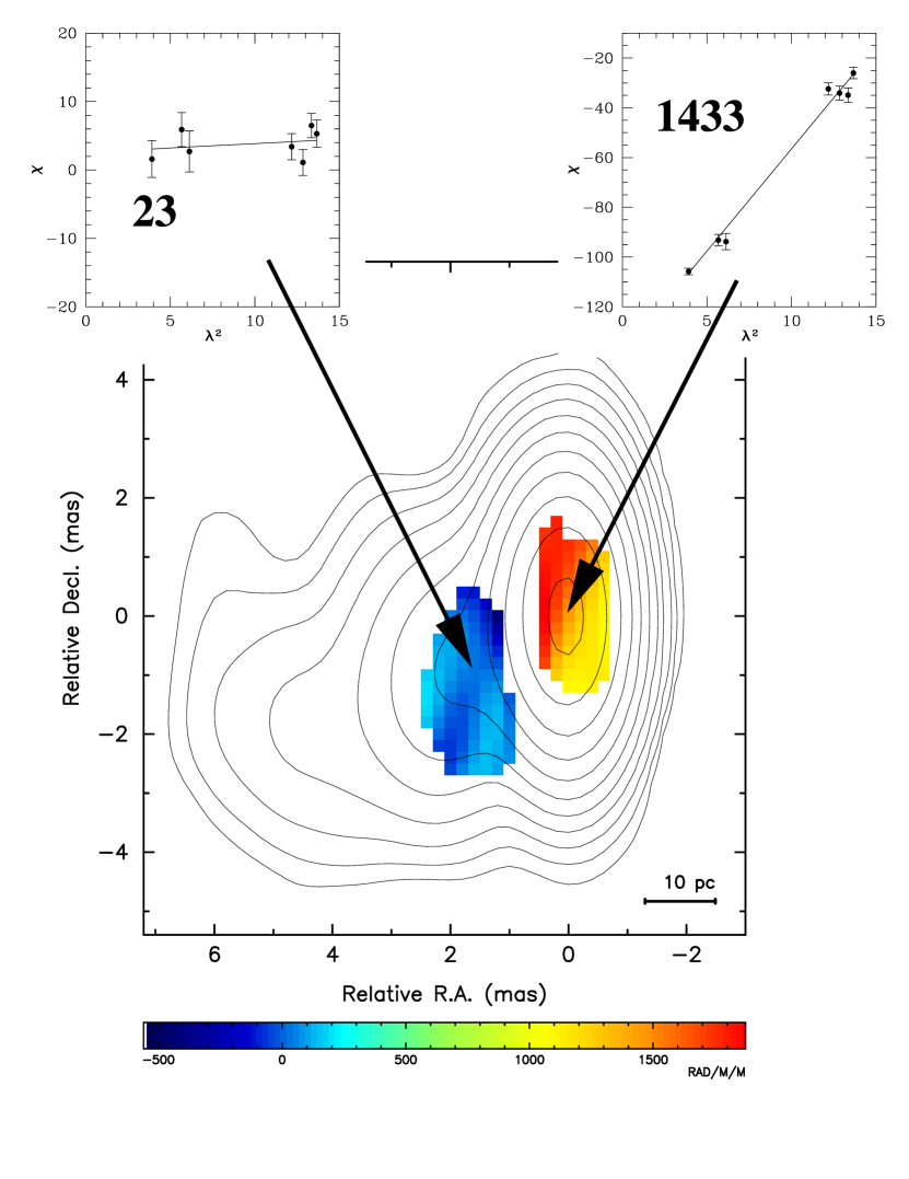
Figure 15: (a) Rotation measure image (color) for 0748+126 overlaid on Stokes I contours at 15 GHz. The inset is a plot of EVPA $\chi$ (deg) versus $\lambda^{2}$ (cm²). (b) Electric vectors (1 mas = 17 mJy beam^-1 polarized flux density) corrected for Faraday Rotation overlaid on Stokes I contours. Contours start at 1.2 mJy beam^-1 and increase by factors of two.

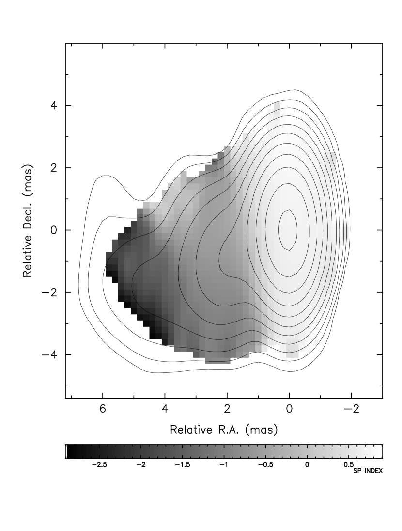
Figure 16: Spectral index $\alpha_{12.1}^{8.1}$ plot for 0748+126 overlaid on Stokes I contours at 15 GHz. Contours start at 1.2 mJy beam^-1 and increase by factors of two.

A typical quasar core RM of 1433 $\pm$ 34 rad m^-2 and jet RM consistent with 0 (23 $\pm$ 40 rad m^-2) are shown in Fig. 15a. These two RM regions have EVPAs which differ by $\approx$ 45^∘ (Fig. 15b). Fig. 16 shows the typical flat spectrum core and steep spectrum jet. Wills & Wills (1976) report an uncertainty in the published redshift.

3.9 B1055+018

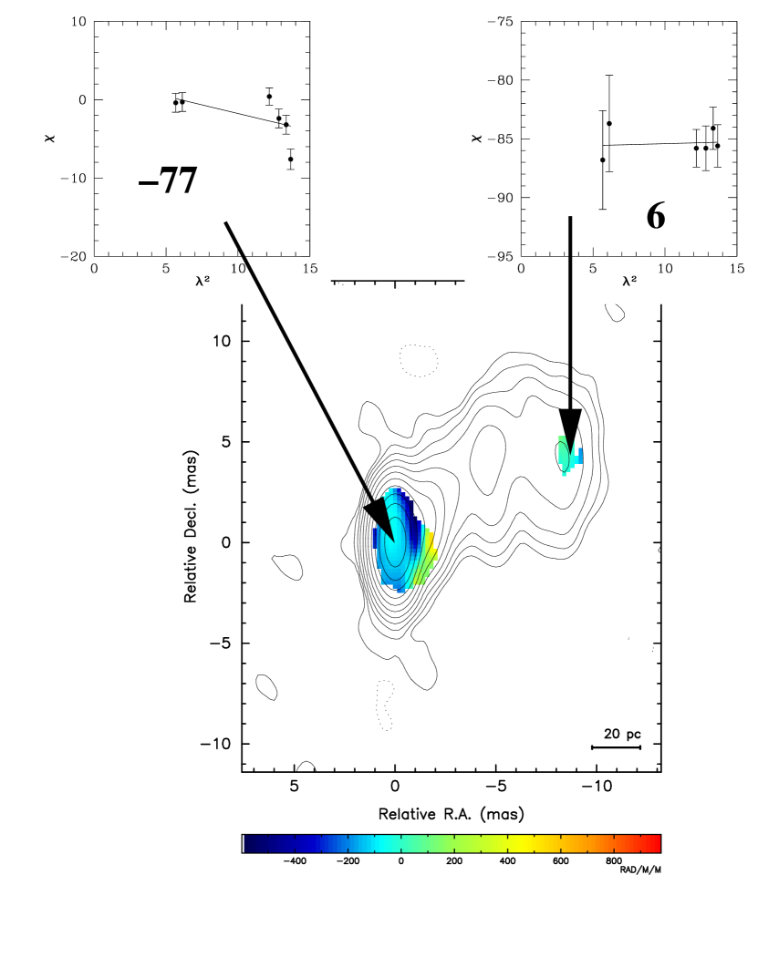
Figure 17: (a) Rotation measure image (color) for 1055+018 overlaid on Stokes I contours at 12.5 GHz. The inset is a plot of EVPA $\chi$ (deg) versus $\lambda^{2}$ (cm²). (b) Electric vectors (1 mas = 25 mJy beam^-1 polarized flux density) corrected for Faraday Rotation overlaid on Stokes I contours. Contours start at 2.4 mJy beam^-1 and increase by factors of two.

An error in the observing schedule caused the loss of the 15 GHz data for 1055+018, so the total intensity contours in Figs 17a & b, and Fig. 18 are for 12.5 GHz. Table 4 shows the core of this BL Lacertae object is relatively weakly polarized at 8.1 GHz, and the core and jet RMs ($-77\pm 25$ and $6\pm 73$ rad m^-2) are consistent with zero. Approximately 50% of pixels have a reduced $\chi^{2}$ which is not consistent with a $\lambda^{2}$ law. For the same reason we reject the $\lambda^{2}$ law for the jet of 1055+018. The core is optically thick and the jet component 9 mas NW of the core is optically thin. The jet does not exhibit the interesting “spine & sheath” polarization structure found by Attridge, Roberts, & Wardle (1999) at 5 GHz. Our observations probably lack the sensitivity to reveal the sheath structure which Attridge, Roberts & Wardle observed.

3.10 3C 279

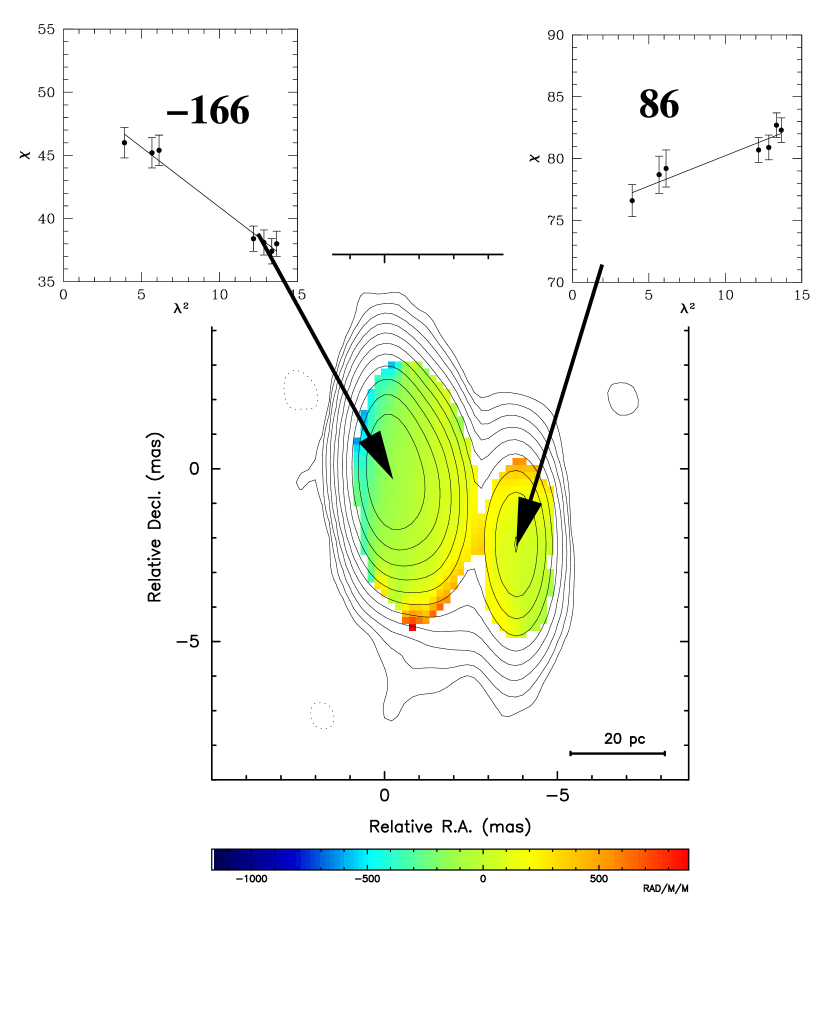
Figure 19: (a) Rotation measure image (color) for 3C 279 overlaid on Stokes I contours at 15 GHz. The inset is a plot of EVPA $\chi$ (deg) versus $\lambda^{2}$ (cm²). (b) Electric vectors (1 mas = 250 mJy beam^-1 polarized flux density) corrected for Faraday Rotation overlaid on Stokes I contours. Contours start at 5.3 mJy beam^-1 and increase by factors of two.

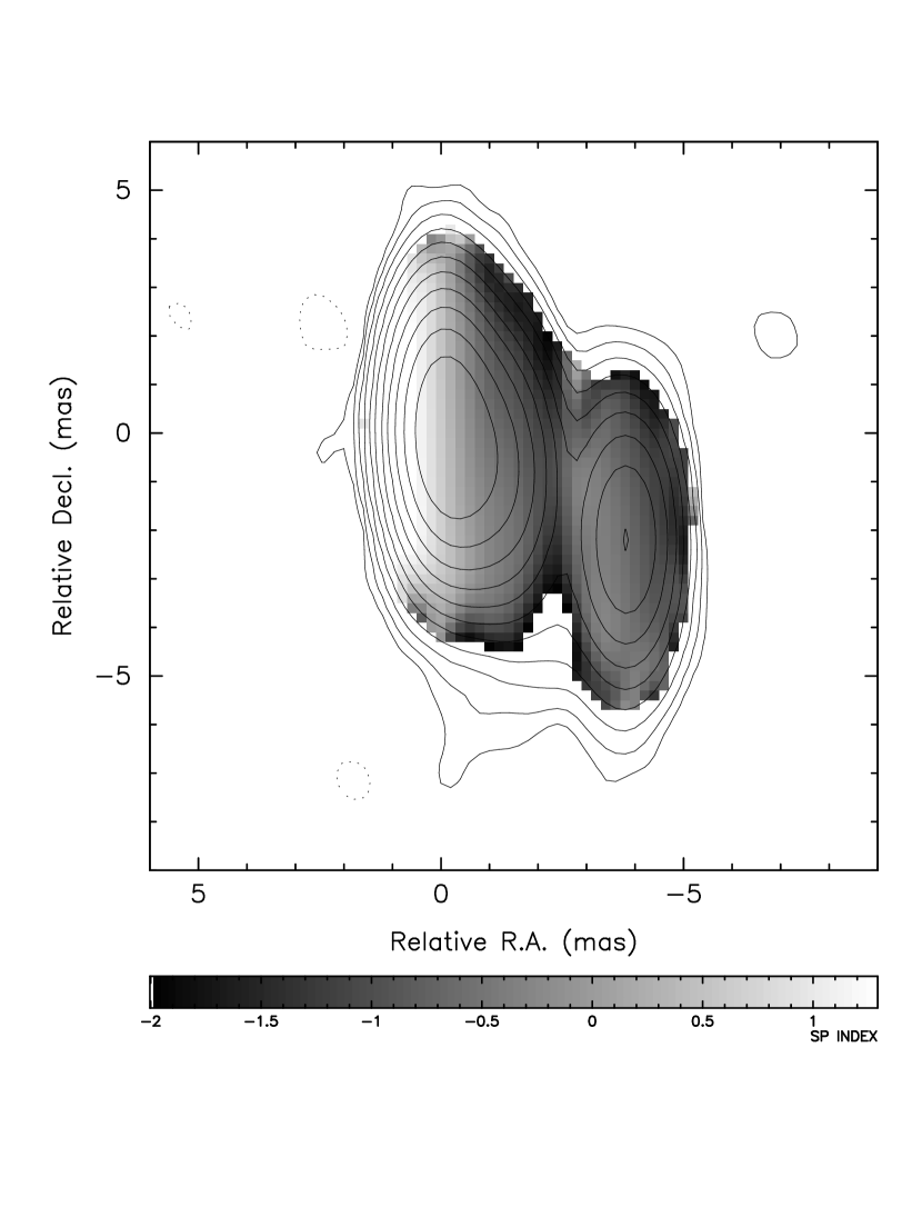
Figure 20: Spectral index $\alpha_{12.1}^{8.1}$ plot for 3C 279 overlaid on Stokes I contours at 15 GHz. Contours start at 5.3 mJy beam^-1 and increase by factors of two.

This paper presents the fifth epoch of RM monitoring for the quasar 3C 279. Previous epochs were presented in Taylor (1998, 2000) and Zavala & Taylor (2001, 2003). The core RM (Fig. 19a) is $-$166 $\pm$ 19 rad m^-2 and component C4 (4 mas west of the core) has an RM 86 $\pm$ 21 rad m^-2. The RM corrected EVPA (Fig. 19b) of the core is 50^∘ and for C4 is 76^∘. Within a milliarcsecond of the core the spectral index becomes negative (Fig. 20).

3.11 B1546+027

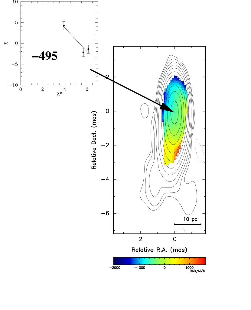
Figure 21: (a) Rotation measure image (color) for 1546+027 overlaid on Stokes I contours at 15 GHz. The inset is a plot of EVPA $\chi$ (deg) versus $\lambda^{2}$ (cm²). (b) Electric vectors (1 mas = 67 mJy beam^-1 polarized flux density) corrected for Faraday Rotation overlaid on Stokes I contours. Contours start at 1.2 mJy beam^-1 and increase by factors of two.

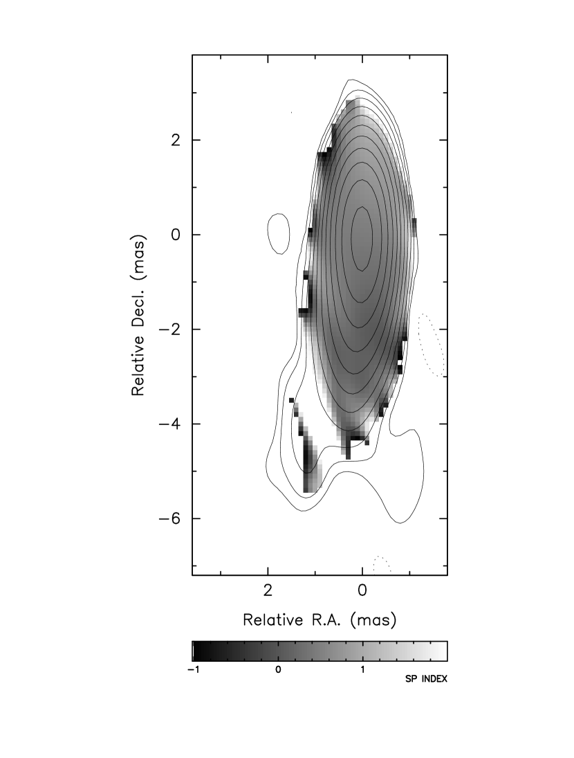
Figure 22: Spectral index $\alpha_{15.1}^{12.5}$ plot for 1546+027 overlaid on Stokes I contours at 15 GHz. Contours start at 1.2 mJy beam^-1 and increase by factors of two.

A error in the observation caused the loss of the 8 GHz data for 1546+027. The RM in the core (Fig. 21a) of $-$495 $\pm$ 105 rad m^-2 is over 15 and 12 GHz only. There is a change in the RM corrected EVPA from N$-$S as one proceeds along the jet (Fig. 21b). Fig. 22, the spectral index map, shows that 1546+027 has an inverted spectrum up to 15 GHz.

3.12 B1548+056

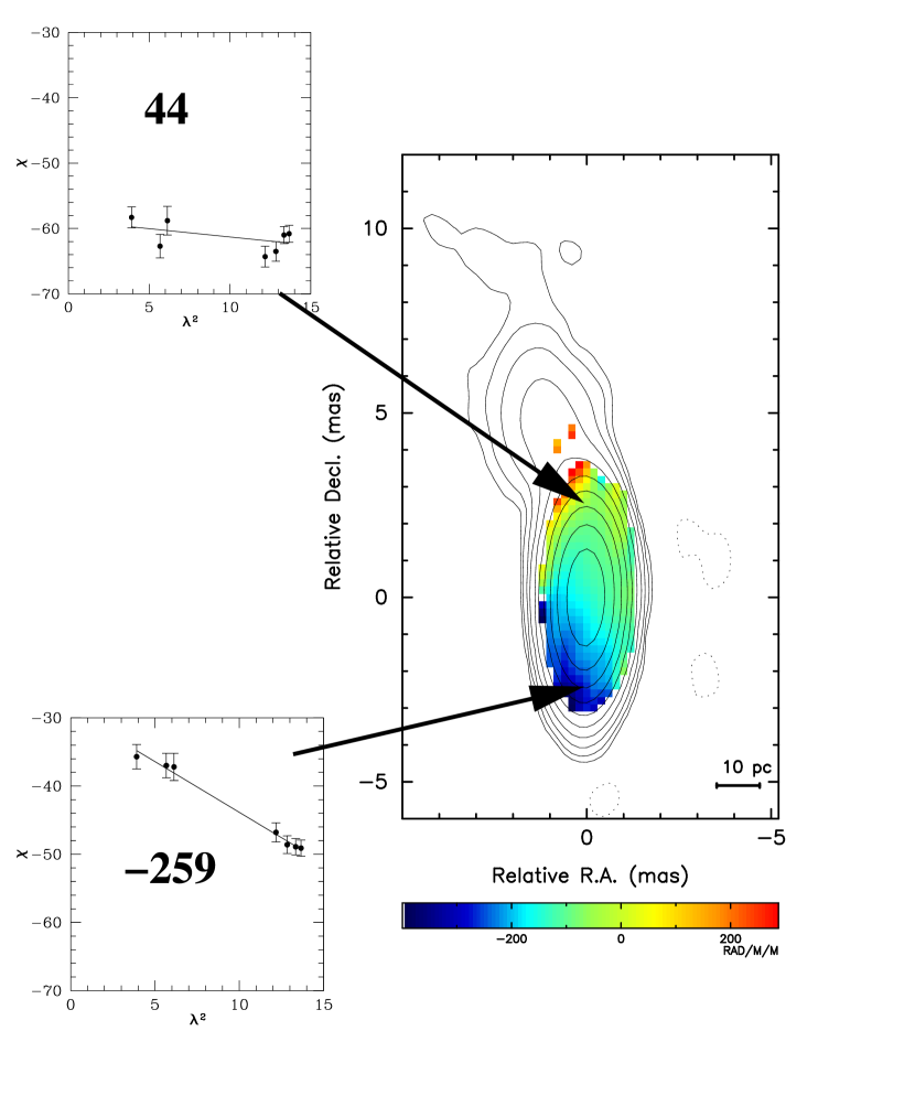
Figure 23: (a) Rotation measure image (color) for 1548+056 overlaid on Stokes I contours at 15 GHz. The inset is a plot of EVPA $\chi$ (deg) versus $\lambda^{2}$ (cm²). (b) Electric vectors (1 mas = 50 mJy beam^-1 polarized flux density) corrected for Faraday Rotation overlaid on Stokes I contours. Contours start at 2.4 mJy beam^-1 and increase by factors of two.

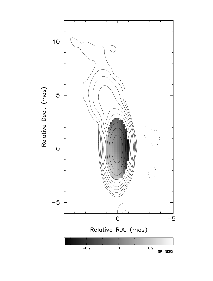
Figure 24: Spectral index $\alpha_{12.1}^{8.1}$ plot for 1548+056 overlaid on Stokes I contours at 15 GHz. Contours start at 2.4 mJy beam^-1 and increase by factors of two.

A gradient in rotation measure is visible across 1548+056 from south$-$north in Fig. 23a. Three mas south of the peak the RM is $-$259 $\pm$ 27 rad m^-2, while 3 mas north of the peak the RM has declined to 44 $\pm$ 59 rad m^-2. This occurs over a projected distance of less than 60 pc. The RM corrected electric vectors maintain a roughly constant orientation across the source (Fig. 23b). There is a flat spectral index along the RM gradient as shown in Fig. 24.

3.13 B1741$-$038

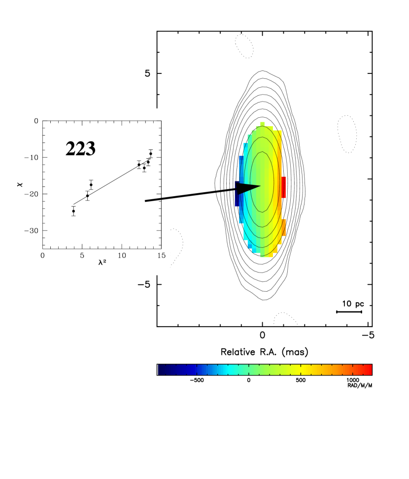
Figure 25: (a) Rotation measure image (color) for 1741$-$038 overlaid on Stokes I contours at 15 GHz. The inset is a plot of EVPA $\chi$ (deg) versus $\lambda^{2}$ (cm²). (b) Electric vectors (1 mas = 100 mJy beam^-1 polarized flux density) corrected for Faraday Rotation overlaid on Stokes I contours. Contours start at 5.4 mJy beam^-1 and increase by factors of two.

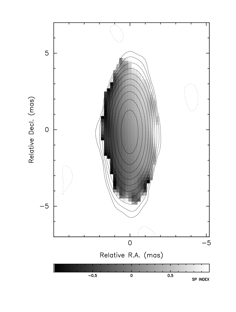
Figure 26: Spectral index $\alpha_{12.1}^{8.1}$ plot for 1741$-$038 overlaid on Stokes I contours at 15 GHz. Contours start at 5.4 mJy beam^-1 and increase by factors of two.

1741$-$038 was one of the first three sources detected with a Space VLBI experiment (Levy et al., 1986). This quasar is essentially unresolved (Fig. 25a), and has a core RM of 223 $\pm$ 20 rad m^-2. The RM corrected electric vectors are oriented along a SE-NW axis (Fig. 25b). The spectrum steepens from S$-$N as shown in Fig. 26.

3.14 B1749+096

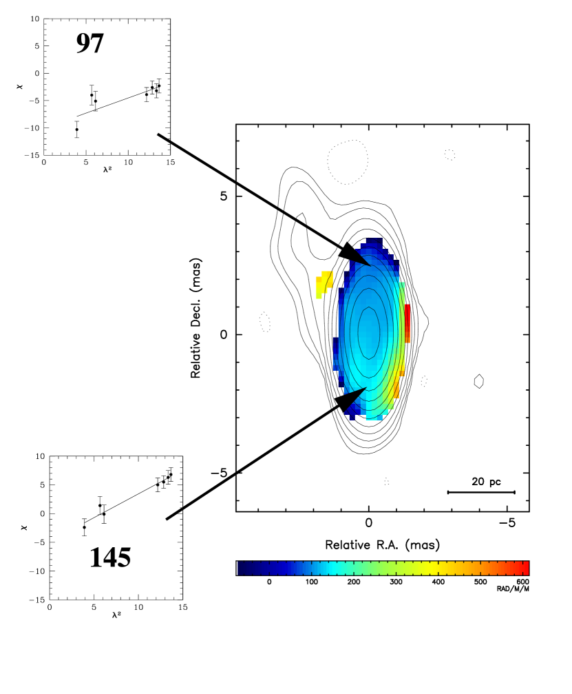
Figure 27: (a) Rotation measure image (color) for 1749+096 overlaid on Stokes I contours at 15 GHz. The inset is a plot of EVPA $\chi$ (deg) versus $\lambda^{2}$ (cm²). (b) Electric vectors (1 mas = 67 mJy beam^-1 polarized flux density) corrected for Faraday Rotation overlaid on Stokes I contours. Contours start at 2.1 mJy beam^-1 and increase by factors of two.

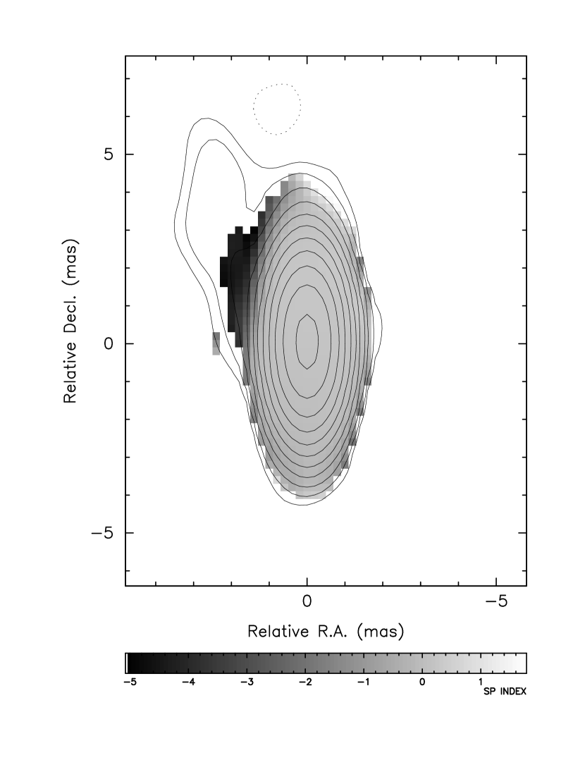
Figure 28: Spectral index $\alpha_{12.1}^{8.1}$ plot for 1749+096 overlaid on Stokes I contours at 15 GHz. Contours start at 2.1 mJy beam^-1 and increase by factors of two.

The BL Lac object 1749+096 has a fairly uniform RM distribution. The fits in the inset plots of Fig. 27a have RMs of 145 $\pm$ 24 rad m^-2 and 97 $\pm$ 25 rad m^-2, which are essentially the same within the errors. The RM corrected electric vectors appear roughly perpendicular to the projected direction of the jet (Fig. 27b). 1749+096 is dominated by a flat spectrum core (Fig. 28), thus the magnetic vectors are parallel to the electric vectors (Aller, 1970) in Fig. 27b.

3.15 B2021+317

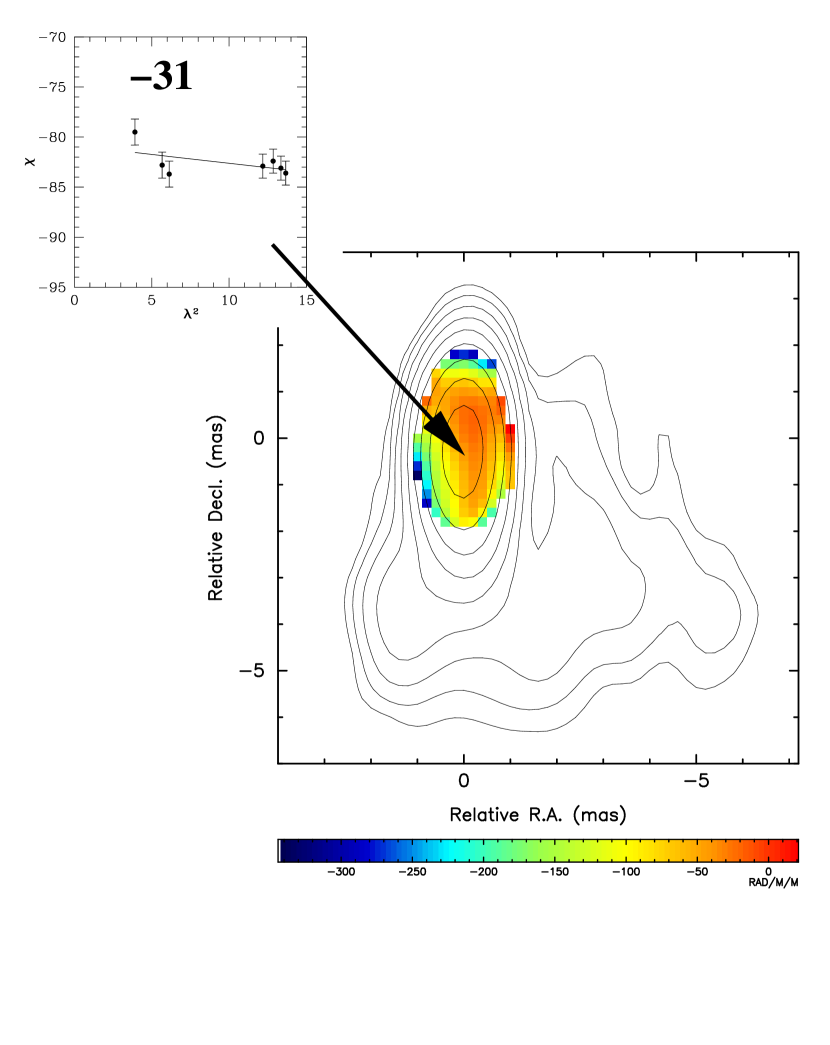
Figure 29: (a) Rotation measure image (color) for 2021+317 overlaid on Stokes I contours at 15 GHz. The inset is a plot of EVPA $\chi$ (deg) versus $\lambda^{2}$ (cm²). (b) Electric vectors (1 mas = 12.5 mJy beam^-1 polarized flux density) corrected for Faraday Rotation overlaid on Stokes I contours. Contours start at 1.2 mJy beam^-1 and increase by factors of two.

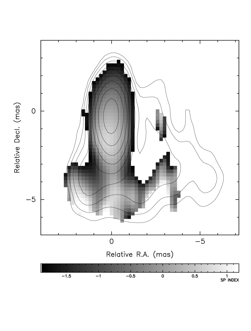
Figure 30: Spectral index $\alpha_{12.1}^{8.1}$ plot for 2021+317 overlaid on Stokes I contours at 15 GHz. Contours start at 1.2 mJy beam^-1 and increase by factors of two.

This source lacks an optical counterpart, and has an RM consistent with zero ($-$31 $\pm$ 21 rad m^-2) in Fig 29a. The NRAO VLA Sky Survey (NVSS; Condon et al., 1998) image shows a jet extending 2 arcminutes to the NE, an extreme misalignment with the structure seen on parsec scales. The jet has a very diffuse and poorly ordered structure. The RM corrected electric vectors are oriented E-W (Fig 29b). The core is optically thick (Fig. 30), and the magnetic vectors are therefore parallel to the electric vectors in Fig 29b.

3.16 B2201+315

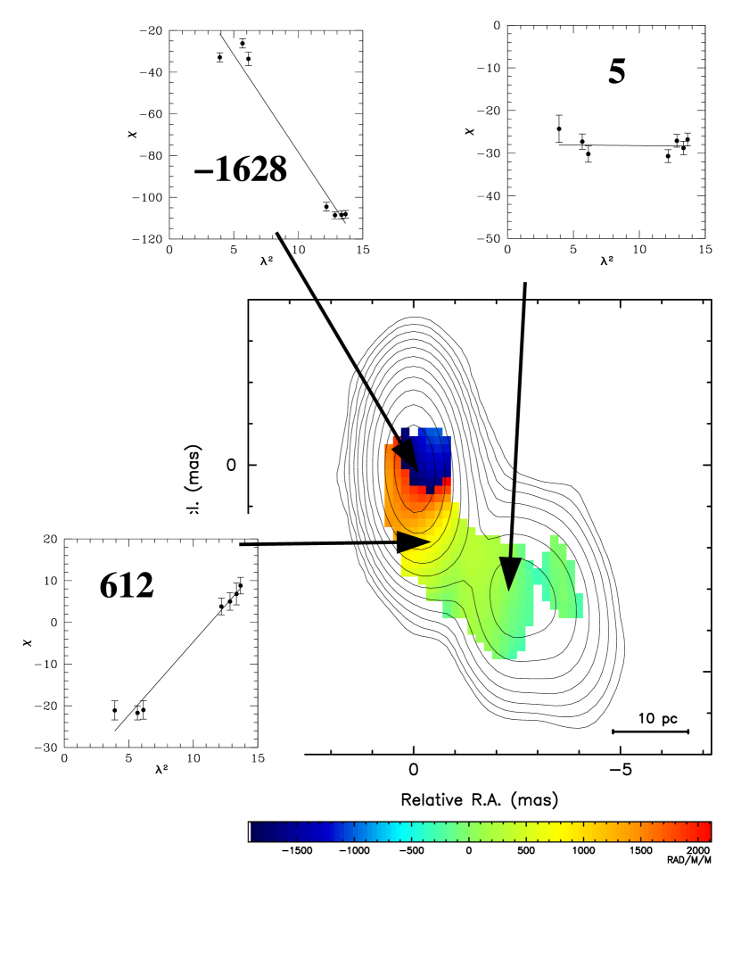
Figure 31: (a) Rotation measure image (color) for 2201+315 overlaid on Stokes I contours at 15 GHz. The inset is a plot of EVPA $\chi$ (deg) versus $\lambda^{2}$ (cm²). (b) Electric vectors (1 mas = 10 mJy beam^-1 polarized flux density) corrected for Faraday Rotation overlaid on Stokes I contours. Contours start at 1.2 mJy beam^-1 and increase by factors of two.

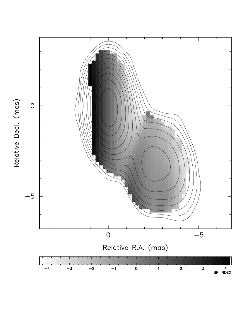
Figure 32: Spectral index $\alpha_{12.1}^{8.1}$ plot for 2201+315 overlaid on Stokes I contours at 15 GHz. Contours start at 1.2 mJy beam^-1 and increase by factors of two.

There is a sign change in the slope of the RM across the core of this quasar from $-$1628 $\pm$ 36 to 612 $\pm$ 36 rad m^-2 (Fig. 31a). RM corrected electric vectors appear in Fig. 31b. The 12 and 15 GHz position angles in the core do not appear to follow the slope set by the 8 GHz position angles. This may result from optical depth effects as the core is optically thick (Fig. 32). Nearly half of the pixels of the core have a reduced $\chi^{2}$ greater than the $3\sigma$ level. Beyond 2 mas SW of the core the RM fit $\chi^{2}$ do become consistent with a $\lambda^{2}$ law. Four mas southwest of the core the RM has decreased to 5 $\pm$ 33 rad m^-2, or consistent with zero.

3.17 3C 446

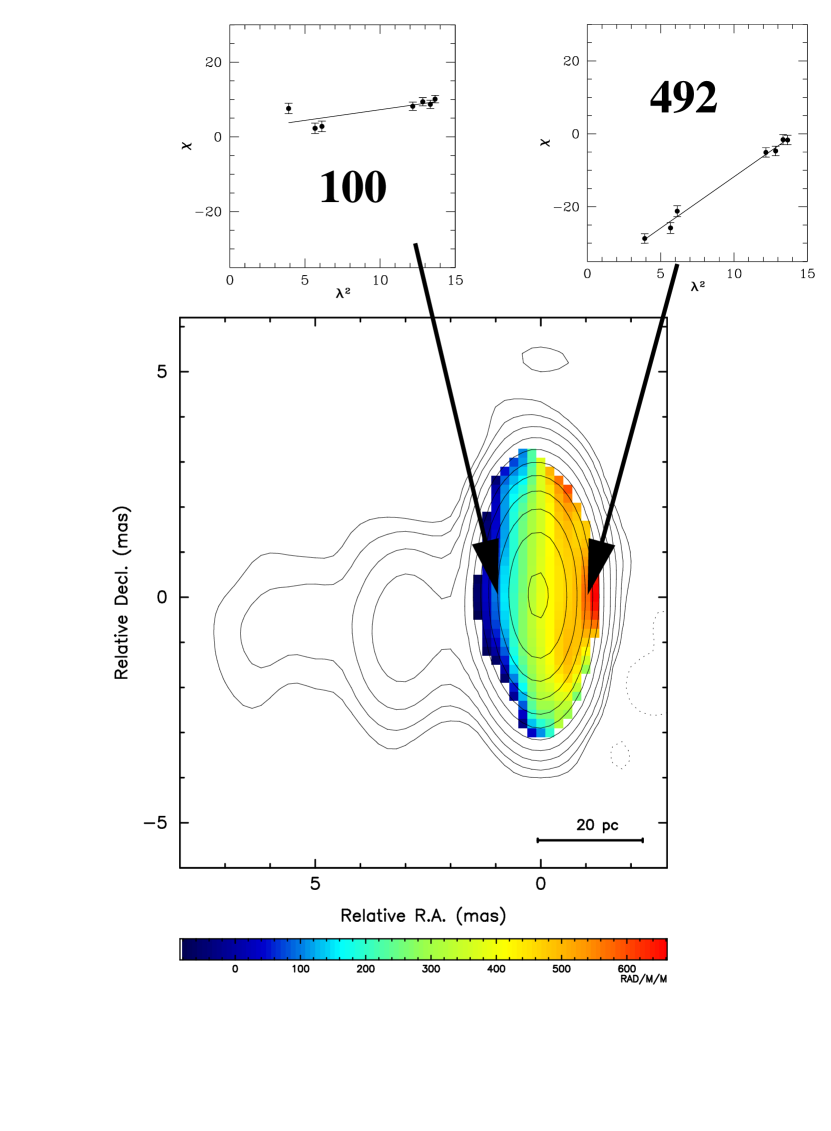
Figure 33: (a) Rotation measure image (color) for 3C 446 overlaid on Stokes I contours at 15 GHz. The inset is a plot of EVPA $\chi$ (deg) versus $\lambda^{2}$ (cm²). (b) Electric vectors (1 mas = 200 mJy beam^-1 polarized flux density) corrected for Faraday Rotation overlaid on Stokes I contours. Contours start at 5.1 mJy beam^-1 and increase by factors of two.

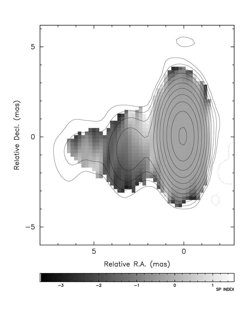
Figure 34: Spectral index $\alpha_{12.1}^{8.1}$ plot for 3C 446 overlaid on Stokes I contours at 15 GHz. Contours start at 5.1 mJy beam^-1 and increase by factors of two.

3C 446 could be a transition object between the quasar and BL Lacertae objects (Falomo, Scarpa, & Bersanelli, 1994), but the case for a quasar identification has also been made by Bregman et al. (1986) and Bregman et al. (1988). In Fig. 33a the RM decreases from 492 $\pm$ 23 rad m^-2 west of the core to 100 $\pm$ 22 rad m^-2 east of the core. This gradient in RM tracks a change in the RM corrected electric vector direction of almost 60^∘ (Fig. 33b). 3C 446 has a flat, optically thick spectrum throughout its RM distribution (Fig. 34). The jet, which has no detected polarized flux, is optically thin.

4 Discussion

To characterize the RM distribution of the various sources we consider the RM value of the cores of the AGN presented here. Fig. 35 shows the histogram of the observed core RM in 200 rad m^-2 bins. Although this is the RM at a single pixel, it is generally representative of the values found in the flat spectrum cores of the individual AGN. As expected there is no preference to the sign of the RM, and the mean RM observed is 137 rad m^-2. The sparse sampling prevents a reliable determination of the distribution function, but the general appearance is consistent with a zero mean Gaussian distribution. To understand the magnitude of the parsec scale RM effect we determined the average of the absolute value of the observed core RM. This average absolute value, 644 rad m^-2, is approximately twice the maximum of about 300 rad m^-2 expected on larger angular scales from the observed rotation measures in Simard-Normandin, Kronberg, & Button (1981).

4.1 RM and Radio Luminosity

Our understanding of AGN is based largely on an empirical foundation which suggests a differentiation based on luminosity (Lawrence, 1987). We attempt to test for this differentiation by plotting the rest frame core RM versus 15 GHz radio luminosity in Fig. 36. The cosmology used was $\Omega_{m}$ = 0.23, $\Omega_{vac}$ = 0.77, and H₀ = 75 km sec^-1 Mpc^-1. We made use of E. L. Wright’s online cosmology calculator to determine the luminosity distance, and allowed for relativistic beaming by using a unit solid angle. Fig. 36 looks like a scatter plot, but an interesting fact emerges. The multi-epoch data for 3C 279 shows that the rotation measure is relatively insensitive to luminosity. At a given radio luminosity 3C 279 has high and low rotation measures. Whatever causes the change in rotation measure in the core of 3C 279 does not require large changes in the radio luminosity.

The intrinsic rotation measure and radio luminosity are both redshift dependent properties. Therefore, a false correlation is expected in Fig. 36. As the plot resembles a scatter plot the false correlation from plotting two redshift dependent quantities versus each other does not appear significant. To quantify this we used the ASURV Revision 1.2 statistics package (Lavalley, Isobe, & Feigelson, 1992). We used the Cox and generalized Kendall’s $\tau$ tests (Isobe, Feigelson, & Nelson, 1986) to test for a radio luminosity$-$intrinsic RM correlation. The Cox test gives the probability of no correlation at the 20% level, and the Kendall’s $\tau$ rules out a correlation at the 5% level. We conclude that there is no correlation between the intrinsic RM and radio luminosity even though one might be expected.

4.2 Fractional polarization properties

Faraday rotation by a foreground screen can produce beam depolarization (Gardner & Whiteoak, 1966). Longer wavelengths will exhibit this effect to a higher degree due to the $\lambda^{2}$ nature of Faraday rotation. Fig. 37a shows the 15 GHz core fractional polarization versus observed rotation measure for the sources in Table 4. There is a lack of sources with high core fractional polarization and high observed rotation measure. This distinction is somewhat more pronounced at 8 GHz as seen in Fig. 37b. In Zavala & Taylor (2003) we noted that an RM gradient of 770 rad m^-2 across a beam is sufficient to cause substantial depolarization at 8 GHz. To more quantitatively account for the observed fractional polarization the beam depolarization can be modeled in the same manner as depolarization due to internal Faraday rotation (Gardner & Whiteoak, 1966). The observed fractional polarization is a sinc function of the rotation measure. By fixing $\lambda^{2}$ and varying the RM we can plot the expected beam depolarization, but this requires setting an amplitude to the sinc function at zero RM. We set this amplitude at 10%, in agreement with the maximum observed fractional polarization at 8 GHz for this small sample. This is similar to the maximum core fractional polarization at 5 GHz found for 106 quasars by Pollack, Taylor, & Zavala (2003). In Fig. 37a & b the solid line plots the expected beam depolarization using the equation

$$\rm{m(\%)}=10|sinc(RM\lambda^{2})|$$ (3)

as derived by Burn (1966). This is a simple model of a constant gradient across the beam. Fig. 37b appears to agree with the expected 8 GHz beam depolarization. The 15 GHz fractional polarization data seem to respond to the expected depolarization more strongly. The first null in fractional polarization for 15 GHz in this simple model is not expected to occur until an RM gradient of almost 8000 rad m^-2. Yet the fractional polarization is 2% or less at 2000 rad m^-2. This indicates that the real situation is more complicated than a constant RM gradient in a foreground screen.

Tribble (1991) put forth a modification to the treatment of Burn by considering variations in the rotation measure which are comparable to the resolution of the telescope. His results increase the fractional polarization as compared to the Burn model, and so would not help a foreground gradient to explain together the 8 and 15 GHz fractional polarization data.

Surprisingly, the maximum core fractional polarizations of our 8 GHz data presented here, and at 5 GHz from Pollack, Taylor, & Zavala (2003) are higher than the 6% found by Lister (2001) at 43 GHz. One might expect that the decreased depolarization and less blending of components at 43 GHz would yield higher core fractional polarizations than observed at lower frequencies.

Multi-epoch monitoring of the RM structure in 3C 279 allows us to revisit the idea of a luminosity/RM correlation. Fig. 38 shows the results from five years of rotation measure data for the core of the quasar 3C 279. The solid line in Fig. 38 shows the observed core rotation measure versus epoch. The 8 and 15 GHz core fractional polarization are shown as dashed and dash-dot lines respectively. What is immediately evident is the anti-correlation between the core fractional polarization at 8 and 15 GHz, and the observed core rotation measure. From Table 4 we see that the highest rotation measure and lowest fractional polarizations occur when the quasar has the highest radio luminosity. This may also be seen in the optical monitoring data of taken at Foggy Bottom Observatory of Colgate University (Balonek & Kartaltepe, 2002, 2004). From January 1997 to June 2001 3C 279 brightened from an R magnitude of 15.5 to 13.6, reaching almost to magnitude 12.5 by August 2001. Superimposed on this trend is considerable variability on time scales of days, as well as microvariability. Overinterpreting the better time-sampled optical light curve should be discouraged, but a relation between the radio and optical luminosity and the varying rotation measure deserves further scrutiny.

4.3 Identification of the Faraday Screen

Faraday rotation serves as a probe of the physical conditions responsible for the observed rotation, but this is only useful if the screen can be identified. We first consider and rule out several locations in order of increasing distance from the supermassive black hole. We then make the argument that the screen is located close to the relativistic jet itself.

The broad emission line region (BLR) is not a likely candidate for the foreground Faraday screen. The BLR is thought to be less than a parsec with a small (1%) volume filling factor $\epsilon$ (Osterbrock, 1989) and cannot account for Faraday affects which appear on scales of tens of parsecs. Reverberation mapping in AGN provides similar size constraints for the BLR (Kaspi et al., 2000). Additionally, the multi-epoch RM maps of 3C 279 can be used to rule out the BLR as a source of variations in the core RM of this blazar. Koratkar et al. (1998) have shown that the Lyman$\alpha$ line in 3C 279 does not track variations in the optical continuum over an eight year period. This implies that as the optical continuum varies any Faraday depth due to the BLR clouds would remain constant. Although the sampling interval of Koratkar et al. (1998) did not coincide with our rotation measure monitoring, it seems reasonable to accept this finding and disregard the BLR as a Faraday screen candidate.

Proceeding out from the center of an AGN the next viable candidate for the Faraday screen is the narrow emission line region (NLR), or the thermal gas expected to confine the NLR clouds. In Zavala & Taylor (2003) and Zavala & Taylor (2002) we ruled out the NLR clouds as a Faraday screen based on similar volume filling factor arguments used to eliminate the BLR clouds. If the NLR clouds are confined in the vicinity of the jet this eliminates the volume filling factor argument.

The hot rarefied gas which confines the NLR clouds is ruled out as the observed RM distributions in individual sources do not exhibit a zero-mean Gaussian distribution (Zavala & Taylor, 2003). Even with this in mind, we examined the possibility of such a stochastic screen using the results of Melrose & MacQuart (1998). Melrose & MacQuart predict that the variance of the Stokes parameters Q and U should decrease as exp($-\lambda^{4}$) in the presence of a stochastic foreground Faraday screen, while the expectation value $<Q^{2}+U^{2}>$ should remain constant. This decrease in Q and U, while $<Q^{2}+U^{2}>$ remains constant, is termed the polarization covariance by Melrose & MacQuart. We examined polarization covariance for the quasar 1611+343 whose RM distribution appears in Zavala & Taylor (2003). The spatial sampling of the RM distribution for this quasar was fairly good, and we found that the variance in Q and U increased with wavelength. The polarization covariance remained constant, or possibly increased slightly. This is further evidence against a purely random Faraday screen.

The accumulating rotation measure observations reinforce the conclusion of Udomprasert et al. (1997) that the Faraday screen cannot be located in the ISM or IGM, and we do not consider this suggestion further.

Essentially by process of elimination we are left to consider a Faraday screen in close proximity to the relativistic jets of AGN. This has important implications for probing the physics of relativistic jets. An exciting example is the suggestion by Blandford (1992) that observers search for evidence of helical magnetic fields through observations of a gradient in the rotation measure transverse to a jet axis. Asada et al. (2002) report the detection of an RM gradient across the jet of 3C 273 and interpret this as evidence for the helical magnetic field expected by some theories and simulations.

Interactions between the jets and ambient material in the centers of AGN as described by Bicknell, Saxton & Sutherland (2003) have also been considered (Zavala & Taylor, 2003). A mixing layer described in Zavala & Taylor (2002) and Zavala & Taylor (2003) also has potential as a foreground Faraday screen. Examinations of the relatively rare (Pollack, Taylor, & Zavala, 2003) broad and polarized jets in AGN will be required to settle the identity of the Faraday screen. For example, the interaction model may be tested by observing the alignment of magnetic vectors at the interaction site through shocks, and an increasing fractional polarization due to this alignment relative to regions of the jet upstream from the supposed interaction.

If a turbulent mixing layer is the Faraday screen than an upper limit to the layer thickness is approximately a jet radius. This requirement exists to prevent significant deceleration of the jet due to mass entrainment (DeYoung, 2002; Rosen et al., 1999). Relativistic motion in the jets of quasars and BL Lac objects, and 3C 120 (Gómez et al., 2000) clearly show that deceleration has not occurred. Non-detection of counterjets shows that relativistic beaming is still substantial, and is another indicator that no significant deceleration has taken place. The deceleration argument limits the maximum screen thickness to less than the observed jet radius. The line of sight distance $L$ is constrained to about 10 parsecs or less.

In Zavala & Taylor (2003) an upper limit to $n_{e}$ was set at a few times 10⁴ cm^-3 due to the lack of apparent free$-$free absorption. Recently published electron densities for the narrow line radio galaxy Cygnus A put $n_{e}$ at 300 cm^-3 (Taylor, Tadhunter, & Robinson, 2003), and we consider this a useful lower limit. Thus, it is reasonable to set $n_{e}$ to 1000 cm^-3. With typical jet rotation measures of 100$-$500 rad m^-2 the net line of sight B field is $\sim$ 0.1$-$0.6 $\mu$Gauss for a 1 parsec path length. Should the same path lengths and electron densities be responsible for the core RMs of quasars then the field strengths will be approximately 1$-$4 $\mu$Gauss, for RMs of 1000$-$3000 rad m^-2. However, the assumption of similar physical conditions for the screen within 10 parsecs of the black hole seems unlikely. A gradient in the physical conditions is expected as we proceed closer to the center of activity.

These magnetic fields are surprisingly weak. To be in equilibrium with a thermal gas similar to that in the NLR (T = 10000 K, $n_{e}$ = 1000 cm^-3) would require fields of approximately 200$\mu$G, approximately two orders of magnitude or more than the simple estimates here produce for the B fields. These weak field estimates may present a problem for a dynamically significant helical magnetic field. It is difficult to see how a helical field could be dynamically important for the relativistic jet with field strengths of less than 10 $\mu$G.

4.4 RM Properties and Optical Classification

For some time it has been apparent that optical AGN classification correlates with fractional polarizations. For example, Gabuzda et al. (1992) presented results which showed that the cores of BL Lac objects were more strongly polarized than quasar cores. This result was verified for a larger sample of AGN by Pollack, Taylor, & Zavala (2003). Using arcsecond scale polarization data Saikia (1999) noted that BL Lac objects and core-dominant quasars had higher fractional polarizations than either lobe-dominant quasars or radio galaxies. Saikia attributed this to an orientation effect due to an obscuring torus which depolarized the cores of radio galaxies and lobe-dominant quasars. Based on the high rotation measures found on parsec scales in quasars Taylor (2000) predicted lower core rotation measures in BL Lacs as compared to quasars. This would arise if BL Lacs have their jets more closely aligned to the line of sight, and if the relativistic jet clears out the magneto-ionic gas responsible for the Faraday rotation. Contrary to this expectation BL Lac itself was found to have a non-negligible Faraday rotation (Reynolds, Cawthorne, & Gabuzda, 2001). With this in mind we will examine whether the rotation measure properties of the cores and jets of BL Lacs and quasars are significantly different. Using the values for the peak rest frame rotation measures (last column of Table 4) we see that the quasars and BL Lacs appear to be different. Table 5 shows the number, the mean $\mu$, error of the mean , and the median rest frame rotation measures for quasars and BL Lac objects. For the quasars there are 26 measurements for 21 quasars because of the multi-epoch observations of 3C 273 and 3C 279. As only one radio galaxy has a core rotation measure we exclude this class from consideration. The quasars have a mean rest frame rotation measure three times that observed for the BL Lac objects. The median values, which are less affected by outliers, agree with this result. As expected by Taylor (2000) BL Lacs seem to have a systematically lower core RM compared to quasars. These are small number statistics, and a Kolmogorov-Smirnov test (Press et al., 1992) gives a probability of 0.011 that the BL Lac and quasar core RMs are drawn from the same parent distribution. This is only a 2.5$\sigma$ result. Fig. 39 is a histogram of the rest frame core RM of BL Lacs (angular line boxes) and quasars (open boxes). Clearly small number statistics limit our ability to distinguish any difference between the two AGN classes that might exist based on RM. All we can say is that there is a suggestion that quasar and BL Lac core rotation measures are different, and better statistics are needed to establish this on a firm foundation.

Some shaking to this foundation has already occurred. Mutel & Denn (2003) report in their multi-epoch monitoring of BL Lac an observation of a rotation measure of 6000 rad m^-2. This quasar-like RM further blurs the distinction between the quasars and BL Lac’s which also exists in their optical spectral line properties (Vermeulen et al., 1995). The BL Lac redshift distribution does not extend much beyond a z of 1 (Rector & Stocke, 2001) so we have only a small overlap for quasars and BL Lacs with redshifts less than 1. Our primarily single epoch RM observations may certainly undersample a highly variable phenomenon as Mutel & Denn (2003) and Zavala & Taylor (2001) demonstrate.

The same cannot be said for the jets of BL Lacs and quasars. To define the jets we used the 8-12 GHz spectral index maps, and defined the jets to be the regions where the spectral index map shows the jet is optically thin ($\alpha<-0.5$). The RM maps are blanked retaining pixels where this criteria for $\alpha$ is met, which enables the RM distribution for the predominantly optically thin jet regions to be determined. We further required that this “jet” region be at least one beamwidth from the map peak, the location where the core RM in Table 4 is taken. These criteria limited the number of sources for which we could investigate the jet RM statistics. Table 6 presents the results of this comparison, and the smaller number statistics are immediately apparent. Neither the mean nor the median values appear significantly different. A K-S test was not performed due to the small numbers present in the comparison of jet RM properties. These small number statistics, especially in the case of the BL Lac objects, and the already noted RM variability of BL Lac objects (§ 4.1), leaves these comparisons of core and jet RM properties suspect. A larger sample of RM observations, with good time sampling, is required to confirm that the jet regions are indeed similar while the cores appear different.

4.5 Breaking the $\lambda^{2}$ Faraday Law

As noted in Section 3 the $\lambda^{2}$ law does not seem to be universally applicable. Both 0202+149 and 0420$-$014 are depolarized perhaps through a superposition of components smaller than the beam size, and no fits to a $\lambda^{2}$ law were possible. There are sources for which sufficient polarized flux is detected at all frequencies and a $\lambda^{2}$ law does not seem applicable. Table 7 lists the sources for which agreement to a $\lambda^{2}$ law seems unlikely based on the reduced $\chi^{2}$ obtained for the RM fits. Lack of agreement to the Faraday rotation law may result for several reasons which we now consider.

Almost all sources have cores optically thick to synchrotron emission as shown in the spectral index maps. This is especially true at 8 and 12 GHz. Observations at different frequencies see different $\tau=1$ surfaces which may not have the same intrinsic polarization angle. If this were the case the RM fits in the optically thick cores should always fail to agree with the $\lambda^{2}$ law as the $\lambda=0$ position angles would not agree. This is not true in general, as most sources show good agreement to the $\lambda^{2}$ law even in the optically thick cores. This is especially true for 3C 273 and 3C 279 which show good agreement to the Faraday rotation law in their optically thick cores over several epochs separated by months to year timescales. This is an interesting result as it requires the different $\tau=1$ surfaces to maintain the same polarization angle orientation. It is known that the jets collimate within a small distance from the black hole (Junor, Biretta, & Livio, 1999) and this collimation may also order the magnetic field within this short distance. For the optically thick regions of the jet higher frequencies see farther down the jet and closer to the black hole (Blandford & K$\rm\ddot{o}$nigl, 1979). As the $\lambda^{2}$ law holds in the optically thick regions, then the different $\tau=1$ surfaces, located at different radii from the black hole, must have the same intrinsic polarization angle and hence magnetic field orientation.

There is no consistent observational picture for the sources which do not show good agreement to a $\lambda^{2}$ law based on the reduced $\chi^{2}$ of the RM fits. Comparing Table 7 with Fig. 36 shows that these sources are not systematically brighter or fainter relative to other sources in the sample. Optical class seems unimportant for the moment as BL Lacs and quasars appear in proportion to their representation in the sample as a whole. Opacity effects do not seem to be important as optically thick sources do show good agreement to the Faraday law for most cases. We examined depolarization as a characteristic and find that the depolarization spans a wide range of values for these sources. Fig. 40 shows the depolarization as the ratio of the 15 GHz fractional polarization to the 8 GHz fractional polarization. Arrows in Fig. 40 show the locations of the five sources for which a reduced $\chi^{2}$ is not in agreement with that expected if the Faraday law were true. The most depolarized source in Fig. 40 is 3C 273 (epoch 2000.07) which shows good agreement to a $\lambda^{2}$ law even with a high depolarization ratio. Homan et al. (2002) report that two sources (not included in this sample) also exhibit non-Faraday law behavior, based on variations in polarization angles at two frequencies over several epochs.

5 Conclusions

The rotation measure properties for a sample of over 40 quasars, radio galaxies and BL Lac objects are examined. The core rotation measures in quasars are observed to vary from approximately 500 rad m^-2 to several thousand rad m^-2 within 10 parsecs of the core. Jet rotation measures are typically 500 rad m^-2 or less. The cores of the seven BL Lac objects examined have RMs in their cores and jets similar to quasar jets. Radio galaxies usually have depolarized cores, and exhibit RMs in their jets varying from a few hundred to 10,000 rad m^-2. A gradient in the foreground Faraday screen is invoked to explain the observed depolarization properties of the sample. The Faraday screen is likely located close to the relativistic jet, although its exact nature remains unclear. Observations of broad, polarized jets, are required to further constrain the identity of the Faraday screen. Net line of sight magnetic fields of 0.1$-$0.6 $\mu$Gauss can account for the observed jet rotation measures. If similar physical conditions exist in quasar cores then the field strength required is of order 1 $\mu$Gauss. Agreement to the $\lambda^{2}$ law in the optically thick cores of quasars and BL Lac objects requires a constant magnetic field orientation at different $\tau=1$ surfaces, and thus at different radii from the black hole.

Table 1: Target Sources

Source	Name	Identification	Magnitude	z	$S_{15}$	Scans	$\sigma_{15\rm{GHz}}$	Peak15GHz
(1)	(2)	(3)	(4)	(5)	(6)	(7)	(8)	(9)
0202+149		Q	22.1	0.41	2.29	8	0.4	1.52
0336$-$019	CTA26	Q	18.4	0.85	2.23	9	0.5	2.01
0355+508	NRAO150	EF	$\cdots$	$\cdots$	3.23	7	3.4	6.40
0458$-$020		Q	18.4	2.29	2.33	9	0.3	0.91
0552+398	DA193	Q	18.0	2.37	5.02	7	1.2	3.02
0605$-$085		Q	18.5	0.87	2.80	7	0.8	1.10
0736+017		Q	16.5	0.19	2.58	7	0.4	1.31
0748+126		Q	17.8	0.89	3.25	7	0.3	1.27
1055+018		BL	18.3	0.89	2.15	11	0.8	4.03
1253$-$055	3C 279	Q	17.8	0.54	21.56	7	2.2	8.81
1546+027		Q	18.0	0.41	2.83	8	0.4	1.53
1548+056		Q	17.7	1.42	4.05	8	1.3	1.68
1741$-$038		Q	18.6	1.05	4.06	7	2.1	4.32
1749+096		BL	16.8	0.32	5.58	7	0.6	2.54
2021+317		EF	$\cdots$	$\cdots$	2.02	9	0.3	0.356
2201+315		Q	15.5	0.30	3.10	10	0.3	2.01
2223$-$052	3C 446	BL	17.2	1.40	3.92	8	1.5	4.74

Note. — Col. (1): B1950 source name. Col. (2): Alternate common name. Col. (3): Optical identification from the literature (NED) with Q = quasar, BL = BL Lac object, EF = empty field. Col. (4): Optical magnitude. Col. (5): Redshift. Col. (6): Total flux density at 15 GHz measured by Kellermann et al. (1998). Col. (7): Number of scans. Col. (8): RMS (mJy beam^-1) in 15 GHz untapered map. Col. (9): Peak flux (Jy) in 15 GHz untapered map.

Table 2: EVPA Calibration using 3C 279

Telescope	Freq.	Date	Pol. Flux	$\chi$
	GHz		mJy	Deg.
UMRAO	8.0	20010620	2044	56.6
	14.5	20010625	2058	60.5
VLA	5.0	20010624	1297	64.0
	8.5	20010624	1995	58.2
	22	20010624	2016	57.0
	43	20010624	1889	57.0
VLBA	8.5	20010621	1894	34.0
	15.15	20010621	2147	$-66$

Table 3: Observational Parameters

Frequency	Bandwidth
8.114, 8.209, 8.369, 8.594	8
12.115, 12.591	16
15.165	32

Note. — Frequencies in GHz, bandwidths in MHz

Table 4: Core RM & Polarization Properties

				8 GHz				15 GHz				8 GHz			15 GHz
Source	Name	ID	z	Peak	Integ	PeakPOL		Peak	Integ	PeakPOL	RM0	Rc	mc		Rc	mc	RMi
(1)	(2)	(3)	(4)	(5)	(6)	(7)		(8)	(9)	(10)	(11)	(12)	(13)		(14)	(15)	(16)
0133+476	DA55	Q	0.86	2921	3103	55		3736	3802	50	-1410	0.941	1.88		0.983	1.33	-4878
0202+149		Q	0.41	1664	2016	$<$1.9		1648	1869	3	$\cdots$	0.825	$<$1.1		0.882	0.18	$\cdots$
0212+735		Q	2.37	2229	3125	39		1844	2445	41	-542	0.713	1.75		0.754	2.22	-6155
0336$-$019	CTA26	Q	0.85	1447	1919	15		2191	2512	28	$\cdots$	0.754	1.04		0.873	1.28	$\cdots$
0355+508		EF	$\cdots$	4631	5479	16		7001	7245	126	-1028	0.845	0.35		0.966	1.80	$\cdots$
0415+379	3C111	G	0.05	861	1963	$<$2.0		1537	2263	$<$1.8	$\cdots$	0.439	$<$2.3		0.679	$<$1.2	$\cdots$
0420$-$014		Q	0.92	2035	2377	7		2644	2872	6	$\cdots$	0.856	0.34		0.921	0.23	$\cdots$
0430+052	3C120	G	0.03	1075	3307	$<$2.1		797	2519	4	2082	0.325	$<$1.5		0.316	3.8	2209
0458$-$020		Q	2.29	668	858	3		931	1055	13	$\cdots$	0.779	0.45		0.882	1.40	$\cdots$
0528+134		Q	2.06	2924	3479	11		3100	3439	32	-163	0.840	0.38		0.901	1.03	-1526
0552+398	DA193	Q	2.37	4440	5345	64		3794	4260	38	215	0.831	1.44		0.891	1.00	2442
0605$-$085		Q	0.87	1114	1674	27		1321	1762	45	401	0.665	2.42		0.750	3.41	1402
0736+017		Q	0.19	758	1102	4		1330	1539	8	$\cdots$	0.688	0.53		0.864	0.60	$\cdots$
0748+126		Q	0.89	955	1276	4		1437	1689	16	1442	0.748	0.42		0.851	1.11	5151
0923+392		Q	0.70	8367	10640	104		7179	8959	175	-218	0.786	1.24		0.801	2.44	-630
1055+018		B	0.89	2969	3813	18		4117	4594	96	$\cdots$	0.779	0.61		0.896	2.33	$\cdots$
1226+023	3C273	Q	0.16	13271	26828	38		12341	21571	173	1800	0.495	0.29		0.572	1.40	2422
	3C273	Q	0.16	9500	27955	27		13500	27180	297	-1900	0.340	0.28		0.497	2.20	-2557
1228+126	M87	G	0.00	1042	2180	$<$2.5		1029	1920	$<$1.8	$\cdots$	0.478	$<$2.4		0.536	$<$1.7	$\cdots$
1253$-$055	3C279	Q	0.54	10824	18538	1056		12226	19773	816	-166	0.583	9.76		0.618	6.67	-394
	3C279	Q	0.54	13277	21207	1139		14650	21335	1457	-91	0.626	8.58		0.687	9.95	-216
	3C279	Q	0.54	12860	20402	1024		14070	21980	1238	-166	0.630	7.96		0.640	8.80	-396
	3C279	Q	0.54	17898	23485	336		19865	24766	1344	-310	0.762	1.88		0.802	6.77	-735
	3C279	Q	0.54	9100	$\cdots$	224		17528	22129	700	-1280	$\cdots$	2.46		0.792	3.99	-3036
1308+326		B	1.00	843	1467	29		667	1079	20	113	0.575	3.44		0.618	3.00	452
1546+027		Q	0.41	$\cdots$	$\cdots$	$\cdots$		1630	1900	64	-474	$\cdots$	$\cdots$		0.858	3.93	-982
1548+056		Q	1.42	2108	2426	118		2149	2469	100	-150	0.869	5.55		0.870	4.65	-878
1611+343	DA406	Q	1.40	2630	4377	46		2692	3880	58	-519	0.601	1.75		0.694	2.15	-2989
1641+399	3C345	Q	0.59	4220	$\cdots$	62		4920	$\cdots$	167	-130	$\cdots$	1.47		$\cdots$	3.39	-329
1741$-$038		Q	1.05	4525	4890	72		4923	5212	86	216	0.925	1.59		0.945	1.75	908
1749+096		B	0.32	2347	2437	162		2643	2702	136	122	0.963	6.90		0.978	5.15	213
1803+784		B	0.68	1798	2430	103		1716	2179	86	-201	0.740	5.73		0.788	5.01	-567
1823+568		B	0.66	599	838	31		647	829	45	-128	0.715	5.18		0.780	6.96	-353
1828+487	3C380	Q	0.69	650	$\cdots$	8		1250	$\cdots$	6	-2220	$\cdots$	1.23		$\cdots$	0.48	-6341
1901+319	3C 395	Q	0.64	834	$\cdots$	13		890	$\cdots$	13	300	$\cdots$	1.6		$\cdots$	1.5	807
1928+738		Q	0.30	1970	$\cdots$	19		2310	$\cdots$	6	-1300	$\cdots$	0.96		$\cdots$	0.26	-2197
2005+403		Q	1.74	750	2154	8		1403	2327	21	654	0.348	1.07		0.603	1.50	4911
2021+317		EF	$\cdots$	437	721	18		476	683	16	-31	0.606	4.12		0.697	3.36	$\cdots$
2021+614		G	0.23	1764	3016	$<$2.0		1559	2174	$<$1.5	$\cdots$	0.585	$<$0.11		0.717	$<$0.1	$\cdots$
2134+004		Q	1.93	3240	$\cdots$	140		3170	$\cdots$	183	1120	$\cdots$	4.32		$\cdots$	5.77	9615
2200+420	BL Lac	B	0.07	1969	3277	63		2029	2982	60	-376	0.601	3.20		0.680	2.96	-430
2201+315		Q	0.30	1111	1779	8		2262	2746	11	$\cdots$	0.625	0.72		0.824	0.49	$\cdots$
2223$-$052	3C446	B	1.40	6184	7227	190		5779	6446	215	383	0.856	3.07		0.897	3.72	2206
2230+114	CTA102	Q	1.04	2740	$\cdots$	13		4490	$\cdots$	48	-610	$\cdots$	0.47		$\cdots$	1.07	-2539
2251+158	3C454.3	Q	0.86	5084	9382	66		5509	8442	40	-263	0.542	1.30		0.653	0.73	-910

Note. — This table is also available in the electronic edition of the Journal. The printed edition contains only a sample. Col. (1): B1950 source name. Col. (2): Alternate common name. Col. (3): Optical identification from the literature (NED) with Q = quasar, BL = BL Lac object, EF = empty field. Col. (5): 8.11 GHz Peak flux density (mJy beam^-1). Col. (6) 8.11 GHz Sum of CLEAN components (mJy). Col. (7) 8.11 GHz polarized flux density (mJy beam^-1) at location of peak. Col. (8-10): Same as for 5$-$7, for 15.1 GHz. Col. (11): Observed core RM (rad m^-2 ). Col. (12): 8.11 GHz core dominance. Col. (13): 8.11 GHz core fractional polarization (%). Col. (14$-$15): Same as 12$-$13, for 15.1 GHz. Col. (16): Core rest frame RM (rad m^-2 ).

Table 5: Rest Frame Core RM Properties

Type	Number	$\mu$	$\sigma_{\mu}$	Median
		rad m-2	rad m-2	rad m-2
Quasars	26	2515	106	1862
BL Lacs	6	704	274	441

Table 6: Rest Frame Jet RM Properties

Type	Number	$\mu$	$\sigma_{\mu}$	Median
		rad m-2	rad m-2	rad m-2
Quasars	12	600	43	458
BL Lacs	4	330	20	264

Table 7: Properties of $\lambda^{2}$ Law Breakers

Source	Type	15 GHz Lum	Depol
		W hz-1
0336$-$019	Q	6.3$\times$1026	1.23
0458$-$020	Q	3.1$\times$1027	3.11
0736+017	Q	1.1$\times$1025	1.13
1055+018	B	5.6$\times$1025	3.82
2201+315	Q	1.3$\times$1027	0.68

Figure 1: EVPA calibration versus $\lambda^{2}$ for 3C 279. Filled circles are VLA polarization monitoring data, and open boxes are the VLBA EVPA’s after the turns derived from Table 3 were applied. The solid line represents a least-squares fit for a Faraday rotation $\lambda^{2}$ law to the VLA data including the 5 GHz position angle (not shown). The fit represents an integrated RM of 31 $\pm$ 10 rad m^-2.

Figure 18: Spectral index $\alpha_{12.1}^{8.1}$ plot for 1055+018 overlaid on Stokes I contours at 12.5 GHz. Contours start at 2.4 mJy beam^-1 and increase by factors of two.

Figure 35: Histogram of the RM in the core (rad m^-2) in 200 rad m^-2 bins for the AGN presented here and in Zavala & Taylor (2003).

Figure 36: The rest frame core rotation measure versus luminosity for the AGN in Table 4. Filled circles are quasars, two open circles are the two epochs for 3C 273, open diamonds are five epochs for 3C 279, X’s are BL Lac objects, and the open triangle is the radio galaxy 3C 120. The luminosity distance was determined with $\Omega_{m}$ = 0.23, $\Omega_{vac}$ = 0.77, and H₀ = 75 km sec^-1 Mpc^-1.

Figure 37: (a) Core fractional polarization in percent at 15 GHz for the objects in Table 4 versus observed rotation measure. Filled circles are quasars, open circles are two epochs of 3C 273, open diamonds are 5 epochs of 3C 279, X’s are BL Lac objects, and the open triangle is the radio galaxy 3C 120. (b) Core fractional polarization in percent at 8 GHz for the objects in Table 4 versus observed rotation measure. Symbols are the same as in a. The solid lie represents the expected beam depolarization from a gradient in a foreground Faraday screen using equation  3.

Figure 38: Five year curves of the core RM and fractional polarization for the quasar 3C 279. The solid line shows the RM versus epoch, the dashed line the 15 GHz core fractional polarization (%), and the 8 GHz core fractional polarization (%) is the dash-dot line. Error bars for the fractional polarization estimates are approximately the size of the plotted filled circles. Errors in the RM are only known for the three most recent epochs.

Figure 39: Histogram of the rest frame core RM for quasars (open) and BL Lac objects (angled line).

Figure 40: Histogram of the depolarization, defined as ratio of core fractional polarization at 15 GHz to the core fractional polarization at 8 GHz for all sources in Table 4. Arrows identify the positions of the five sources for which the $\lambda^{2}$ law may not apply based on the reduced $\chi^{2}$ as discussed in the text.

References

- Aller (1970) Aller, H. D. 1970, ApJ, 161, 19
- Asada et al. (2002) Asada, K., Inoue, M., Uchida, Y., Kameno, S., Fujisawa, K., Iguchi, S. & Mutoh, M. 2002, PASJ, 54, L39
- Attridge, Roberts, & Wardle (1999) Attridge, J. M., Roberts, D. H., & Wardle, J. F. C. 1999, ApJ, 518, L87
- Balonek & Kartaltepe (2002) Balonek, T. J. & Kartaltepe, J. S. 2002, Bulletin of the American Astronomical Society, 34, 1109
- Balonek & Kartaltepe (2004) Balonek, T. & Kartaltepe, J. 2004, AJ, in preparation
- Bicknell, Saxton & Sutherland (2003) Bicknell, G. V., Saxton, C. J. & Sutherland, R. S. 2003, Publ. Astron. Soc. Australia, 20, 102
- Blandford (1992) Blandford, R. D. 1992 in Astrophysical Jets, Space Telescope Science Inst. Symp. Ser. 6 (Cambridge: Cambridge University Press) 15
- Blandford & Knigl (1979) Blandford, R. D. & Knigl, A. 1979, ApJ, 232, 34
- Bregman et al. (1986) Bregman, J. N., Glassgold, A. E., Huggins, P. J., & Kinney, A. L. 1986, ApJ, 301, 698
- Bregman et al. (1988) Bregman, J. N. et al. 1988, ApJ, 331, 746
- Burn (1966) Burn, B. J. 1966, MNRAS, 133, 67
- Clements, Jenks & Torres (2003) Clements, S. D., Jenks, A. & Torres, Y. 2003, ApJ, 126, 37
- Condon et al. (1998) Condon, J. J., Cotton, W. D., Greisen, E. W., Yin, Q. F., Perley, R. A., Taylor, G. B., & Broderick, J. J. 1998, AJ, 115, 1693
- Cooper & Price (1962) Cooper, B. F. C. & Price, R. M. 1962, Nature, 195, 1084
- Cotton (1993) Cotton, W. D. 1993, AJ, 106, 1241
- Cotton et al. (1997) Cotton, W. D., Dallacasa, D., Fanti, C., Fanti, R., Foley, A. R., Schilizzi, R. T., & Spencer, R. E. 1997, A&A, 325, 493
- DeYoung (2002) DeYoung, D. S. 2002, The Physics of Extragalactic Radio Sources (Chicago: University of Chicago Press)
- Falomo, Scarpa, & Bersanelli (1994) Falomo, R., Scarpa, R., & Bersanelli, M. 1994, ApJS, 93, 125
- Faraday (1933) Faraday, M. 1933 in Faraday’s Diary, ed. T. Martin (London: G. Bell & Sons), 264
- Gabuzda et al. (1992) Gabuzda, D. C., Cawthorne, T. V., Roberts, D. H., & Wardle, J. F. C. 1992, ApJ, 388, 40
- Gardner & Whiteoak (1966) Gardner, F. F. & Whiteoak, J. B. 1966, ARA&A, 4, 245
- Gómez et al. (2000) Gómez, J., Marscher, A. P., Alberdi, A., Jorstad, S. G., & García-Miró, C. 2000, Science, 289, 2317
- Homan et al. (2002) Homan, D. C., Ojha, R., Wardle, J. F. C., Roberts, D. H., Aller, M. F., Aller, H. D., & Hughes, P. A. 2002, ApJ, 568, 99
- Hutchings et al. (1999) Hutchings 1999, AJ, 117, 1109
- Isobe, Feigelson, & Nelson (1986) Isobe, T., Feigelson, E. D., & Nelson, P. I. 1986, ApJ, 306, 490
- Junor, Biretta, & Livio (1999) Junor, W., Biretta, J. A., & Livio, M. 1999, Nature, 401, 891
- Kaspi et al. (2000) Kaspi, S., Smith, P. S., Netzer, H., Maoz, D., Jannuzi, B. T., & Giveon, U. 2000, ApJ, 533, 631
- Kellermann et al. (1998) Kellermann, K. I., Vermuelen, R. C., Zensus, J. A., & Cohen, M. H. 1998, AJ, 115, 1295
- Koratkar et al. (1998) Koratkar, A., Pian, E., Urry, C. M., & Pesce, J. E. 1998, ApJ, 492, 173
- Lavalley, Isobe, & Feigelson (1992) Lavalley, M., Isobe, T., & Feigelson, E. 1992, ASP Conf. Ser. 25: Astronomical Data Analysis Software and Systems I, 1, 245
- Lawrence (1987) Lawrence, A. 1987, PASP, 99, 309
- Leppänen, Zensus, & Diamond (1995) Leppänen, K. J., Zensus, J. A., & Diamond, P. J. 1995, AJ, 110, 2479
- Levy et al. (1986) Levy, G. S., Linfield, R. P., Ulvestad, J. S., Edwards, C. D., Jordan, J. F. Jr., di Nardo, J., Christensen, C. S., Preston, R. A., Skjerve, L. J., Blaney, K. B. 1986, Science, 234, 187
- Lister (2001) Lister, M. L. 2001, ApJ, 562, 208
- Mattox et al. (1997) Mattox, J. R., Schachter, J., Molnar, L., Hartman, R. C., & Patnaik, A. R. 1997, ApJ, 481, 95
- Melrose & MacQuart (1998) Melrose, D. B. & MacQuart, J.-P. 1998, ApJ, 505, 921
- Moellenbrock et al. (1996) Moellenbrock, G. A. et al. 1996, AJ, 111, 2174
- Mutel & Denn (2003) Mutel, R. L. & Denn, G. R. 2003, to be published in ASP Conf. Ser., Future Directions in High Resolution Astronomy, ed. J. Romney & M. Reid (San Francisco: ASP)
- O’Dea et al. (1990) O’Dea, C. P., Baum, S. A., Stanghellini, C., Morris, G. B., Patnaik, A. R., & Gopal-Krishna 1990, A&AS, 84, 549
- Osterbrock (1989) Osterbrock, D. E. 1989, Astrophysics of Gaseous Nebulae and Active Galactic Nuclei (Mill Valley: University Science Books)
- Perlman et al. (1998) Perlman, E. S., Padovani, P., Giommi, P., Sambruna, R., Jones, L. R., Tzioumis, A., & Reynolds, J. 1998, AJ, 115, 1253
- Press et al. (1992) Press, W. H., Teukolsky, S. A., Vetterling, W. T., & Flannery, B. P. 1992, Numerical Recipes in FORTRAN, (Cambridge: University Press), 2nd ed.
- Pollack, Taylor, & Zavala (2003) Pollack, L. K., Taylor, G. B., & Zavala, R. T. 2003, ApJ, 589, 733
- Pyatunina et al. (2000) Pyatunina, T. B., Marchenko, S. G., Marscher, A. P., Aller, M. F., Aller, H. D., Teräsranta, H., & Valtaoja, E. 2000, A&A, 358, 451
- Rector & Stocke (2001) Rector, T. A. & Stocke, J. T. 2001, AJ, 122, 565
- Reynolds, Cawthorne, & Gabuzda (2001) Reynolds, C., Cawthorne, T. V., & Gabuzda, D. C. 2001, MNRAS, 327, 1071
- Rosen et al. (1999) Rosen, A., Hardee, P. E., Clarke, D. A., & Johnson, A. 1999, ApJ, 510, 136
- Rudnick & Jones (1983) Rudnick, L. & Jones, T. W. 1983, AJ, 88, 518
- Rusk (1988) Rusk, R. E. 1988, Ph.D. Thesis, University of Toronto
- Saikia (1999) Saikia, D. J. 1999, MNRAS, 302, L60
- Schwab & Cotton (1983) Schwab, F. R. & Cotton, W. D. 1983, AJ, 88, 688
- Shepherd (1997) Shepherd, M. C. 1997, in ASP Conf. Ser. 125, Astronomical Data Analysis Software and Systems VI, ed. G. Hunt & H. E. Payne (San Francisco: ASP), 77
- Shepherd, Pearson & Taylor (1994) Shepherd, M. C., Pearson, T. J., & Taylor, G. B. 1994, BAAS, 26, 987
- Simard-Normandin, Kronberg, & Button (1981) Simard-Normandin, M., Kronberg, P. P., & Button, S. 1981, ApJS, 45, 97
- Taylor (1998) Taylor, G. B. 1998, ApJ, 506, 637
- Taylor (2000) Taylor, G. B. 2000, ApJ, 533, 95
- Taylor & Myers (2000) Taylor, G. B. & Myers, S. T. 2000 VLBA Scientific Memo 26, National Radio Astronomy Observatory
- Taylor, Tadhunter, & Robinson (2003) Taylor, M. D., Tadhunter, C. N., & Robinson, T. G. 2003, MNRAS, 342, 995
- Tribble (1991) Tribble, P. C. 1991, MNRAS, 250, 726
- Udomprasert et al. (1997) Udomprasert, P. S., Taylor, G. B., Pearson, T. J., & Roberts, D. H. 1997, ApJ, 483, L9
- Ulvestad, Greisen & Mioduszewski (2001) Ulvestad, J., Greisen, E. W. & Mioduszewski, A. 2001, AIPS Memo 105:AIPS Procedures for initial VLBA Data Reduction, NRAO
- van Moorsel, Kemball, & Greisen (1996) van Moorsel, G., Kemball, A., & Greisen, E. 1996, in Astronomical Data Analysis Software and Systems V, ed. G. H. Jacoby & J. Barnes (San Francisco: ASP), 37
- Vermeulen et al. (1995) Vermeulen, R. C., Ogle, P. M., Tran, H. D., Browne, I. W. A., Cohen, M. H., Readhead, A. C. S., Taylor, G. B., & Goodrich, R. W. 1995, ApJ, 452, L5
- Wardle (1977) Wardle, J. F. C. 1977, Nature, 269, 563
- Wills & Wills (1976) Wills, D. & Wills, B. J. 1976, ApJS, 31, 143
- Zavala & Taylor (2001) Zavala, R. T. & Taylor, G. B. 2001, ApJ, 550, L147
- Zavala & Taylor (2002) Zavala, R. T. & Taylor, G. B. 2002, ApJ, 566, L9
- Zavala & Taylor (2003) Zavala, R. T. & Taylor, G. B. 2003, ApJ, 589, 216