Potential Direct Single-Star Mass Measurement

Abstract

We analyze the lightcurve of the microlensing event OGLE-2003-BLG-175/MOA-2003-BLG-45 and show that it has two properties that, when combined with future high resolution astrometry, could lead to a direct, accurate measurement of the lens mass. First, the lightcurve shows clear signs of distortion due to the Earth’s accelerated motion, which yields a measurement of the projected Einstein radius $\tilde{r}_{\mathrm{E}}$. Second, from precise astrometric measurements, we show that the blended light in the event is coincident with the microlensed source to within about 15 mas. This argues strongly that this blended light is the lens and hence opens the possibility of directly measuring the lens-source relative proper motion $\boldsymbol{\mu}_{\rm rel}$ and so the mass $M=(c^{2}/4G)\mu_{\rm rel}t_{\mathrm{E}}\tilde{r}_{\mathrm{E}}$, where $t_{\mathrm{E}}$ is the measured Einstein timescale. While the lightcurve-based measurement of $\tilde{r}_{\mathrm{E}}$ is, by itself, severely degenerate, we show that this degeneracy can be completely resolved by measuring the direction of proper motion $\boldsymbol{\mu}_{\rm rel}$.

1 Introduction

When microlensing experiments were initiated more than a decade ago (Alcock et al., 1993; Aubourg et al., 1993; Udalski et al., 1993), there was no expectation that the individual lens masses could be determined to much better than an order of magnitude. The only routinely observable parameter, the Einstein timescale $t_{\mathrm{E}}$, is related in a complicated way to the mass $M$ and two other parameters, the lens-source relative parallax, $\pi_{\rm rel}$, and relative proper motion $\mu_{\rm rel}$.

$$t_{\mathrm{E}}=\frac{\theta_{\mathrm{E}}}{\mu_{\rm rel}},$$ (1)

where

$$\theta_{\mathrm{E}}=\sqrt{\kappa M\pi_{\rm rel}}$$ (2)

is the angular radius of the Einstein ring and $\kappa\equiv 4G/(c^{2}\mathrm{AU})\simeq 8.14\,\mathrm{mas}/M_{\odot}$. In principle, therefore, a measurement of $\theta_{\mathrm{E}}$ and $\pi_{\rm rel}$ would lead to a determination of lens mass (Refsdal, 1964). However, since neither $\pi_{\rm rel}$ nor $\mu_{\rm rel}$ are usually known for microlensing events, one can generally obtain only a rough estimate of the lens mass based on statistical inferences from the distance and velocity distributions of the lens and source populations.

The motion of the Earth in its orbit produces a distortion in the observed lightcurve from that of the simple heliocentric case. The magnitude of this distortion is proportional to the size of the projected Einstein radius $\tilde{r}_{\mathrm{E}}$ relative to the size of the Earth’s orbit. This ratio, $\pi_{\mathrm{E}}\equiv\mathrm{AU}/\tilde{r}_{\mathrm{E}}$, is commonly called the microlens parallax, from the similarity in its definition to astrometric parallax. As shown in Gould (2000), $\pi_{\mathrm{E}}\theta_{\mathrm{E}}=\pi_{\rm rel}$, and therefore

$$\pi_{\mathrm{E}}=\sqrt{\frac{\pi_{\rm rel}}{\kappa M}}.$$ (3)

Gould (1992) pointed out that individual lens masses could be determined provided that $\theta_{\mathrm{E}}$ and $\pi_{\mathrm{E}}$ were simultaneously measured for the same event, and he suggested some methods for measuring each. If successfully carried out, microlensing would join only a handful of other methods for directly measuring stellar masses. However, unlike all other methods, microlensing can in principle be used to measure the masses of objects without visible companions, in particular, single stars. At present, the Sun is the only single star whose mass has been directly measured with high precision. This was possible originally only because it has non-stellar, but nevertheless highly visible companions.

In fact, the Sun is also the one single star whose mass has been accurately measured using gravitational lensing. While the original Eddington eclipse experiment was regarded at the time as a confirmation of Einstein’s general relativity (Dyson et al., 1920), general relativity is by this point so well established that this experiment can now be regarded as a mass measurement of the Sun. Applying the same principle to $10^{5}$ stars in the Hipparcos catalog, Froeschle et al. (1997) were able to confirm general relativity (or alternatively measure the mass of the Sun) accurate to 0.3%.

With the notable exception of the Sun, and despite the discovery of several thousand microlensing events as well as a decade of theoretical efforts to invent new ways to measure $\pi_{\mathrm{E}}$ and $\theta_{\mathrm{E}}$, there have been just two mass measurements of single stars using microlensing. The problem is that while the microlens parallax $\pi_{\mathrm{E}}$ has been measured for more than a dozen single lenses (Alcock et al., 1995, 2001; Mao, 1999; Soszyński et al., 2001; Bond et al., 2001; Mao et al., 2002; Smith, Mao & Woźniak, 2002; Bennett et al., 2002; Smith, Mao & Paczyński, 2003; Jiang et al., 2004), the angular Einstein radius $\theta_{\mathrm{E}}$ has been measured for only five single lenses (Alcock et al., 1997, 2001; Smith et al., 2003; Yoo et al., 2004; Jiang et al., 2004). Though Alcock et al. (2001) and Jiang et al. (2004) each measured both $\theta_{\mathrm{E}}$ and $\pi_{\mathrm{E}}$ for their events, respectively MACHO-LMC-5 and OGLE-2003-BLG-238, in neither case was the $\pi_{\mathrm{E}}$ measurement very accurate. Moreover, Gould (2004) showed that the microlens parallax measurement of MACHO-LMC-5 was subject to a discrete degeneracy. Nevertheless, Drake et al. (2004) resolved this degeneracy by a trigonometric measurement of $\pi_{\rm rel}$. Gould et al. (2004) then combined the Drake et al. (2004) measurement of $\pi_{\rm rel}$ and $\boldsymbol{\mu}_{\rm rel}$ with the original photometric data and additional high resolution photometry of the source to constrain the mass to within 17%. This is the most precise direct mass measurement of a single star (other than the Sun) to date. By comparison, the mass of the only other directly measured single star, OGLE-2003-BLG-238, is only accurate to a factor of a few.

An et al. (2002) made the most precise microlens mass measurement to date, with an error of just 9%. However, the lens, EROS-BLG-2000-5, was a binary. In the future, the Space Interferometry Mission should routinely measure the masses of single stars both for stars in the bulge (Gould & Salim, 1999) and for nearby stars passing more distant ones (Refsdal, 1964; Paczyński, 1995; Salim & Gould, 2000). Thus, at present, the direct measurement of single star masses (other than the Sun) remains a difficult undertaking.

Here we present evidence that the microlensing event OGLE-2003-BLG-175/MOA-2003-BLG-45 is an excellent candidate for such a single-star measurement. This seems odd at first sight because, as we will show, $\pi_{\mathrm{E}}$ is measured only to a factor of a few and $\theta_{\mathrm{E}}$ is not measured at all. Hence it would appear difficult to derive any mass measurement, let alone a precise one. However, the event has the relatively unusual property that the lens itself is visible, and this makes a mass measurement possible.

As discussed by Gould (2000) and in greater detail by Gould (2004), $\pi_{\mathrm{E}}$ is actually the magnitude of a vector quantity, $\boldsymbol{\pi}_{\mathrm{E}}$, whose direction is that of the lens-source relative motion. We first show that one component of $\boldsymbol{\pi}_{\mathrm{E}}$ is extremely well determined, so that if its direction could also be constrained, $\pi_{\mathrm{E}}$ would also be well determined. Second, we show that the blended light for this event is almost certainly the lens. We outline how future space-based or possibly ground-based observations could measure $\boldsymbol{\mu}_{\rm rel}$, the vector lens-source relative proper motion (Han & Chang, 2003). When combined with the very well determined $t_{\mathrm{E}}$ for this event, this would yield $\theta_{\mathrm{E}}$ through equation (1). At the same time, such a proper-motion measurement would give the direction of motion and so tightly constrain $\pi_{\mathrm{E}}$.

2 Data

The event [(RA,Dec) = (18:06:34.68, $-$26:01:16.2), $(l,b)=(4.859,-2.550)$] was initially discovered by the Optical Gravitational Lens Experiment (OGLE, Udalski et al. 1994) and was alerted to the community as OGLE-2003-BLG-175 through the OGLE-III Early Warning System (EWS, Udalski 2003) on 2003 May 28. It was independently rediscovered by Microlensing Observations for Astrophysics (MOA, Bond et al. 2001) and designated MOA-2003-BLG-45 on 2003 July 6. It achieved peak magnification on HJD${}^{\prime}\equiv$HJD$-2450000=2863.1$ (2003 August 11).

Observations were carried out by four groups from a total of eight observatories: OGLE from Chile, MOA from New Zealand, the Microlensing Followup Network ($\mu$FUN; Yoo et al., 2004) from Chile and Israel, and the Probing Lensing Anomalies Network (PLANET, Albrow et al. 1998) from Chile, Perth, South Africa and Tasmania. OGLE made a total 178 $I$ band observations from 2001 August 6 to 2003 November 10, of which 119 were during the 2003 season, using the 1.3m Warsaw telescope at the Las Campanas Observatory, Chile, which is operated by the Carnegie Institute of Washington. The exposures were 120 seconds and photometry was obtained using difference image analysis (Woźniak, 2000). MOA made a total of 522 $I$ band observations from 2000 April 12 to 2003 November 4, of which 303 were during the 2003 season, using the 0.6 m Boller & Chivens telescope at Mt. John University Observatory in New Zealand.

$\mu$FUN monitoring of the event began on July 7. Observations were made at the 1.3m (ex-2MASS) telescope at Cerro Tololo InterAmerican Observatory in Chile using ANDICAM (DePoy et al. 2003) and at the Wise 1m telescope at Mitzpe Ramon in Israel using the Wise TeK 1K CCD camera. At CTIO, there were 210 observations in $I$ band, from July 7 to October 29, and 11 observations in $V$, covering a similar period (July 9 – November 5). Exposures were 5 minutes each. Observations at Wise consisted of 12 in $I$ band, covering the period July 8 to August 12, and 56 observations using a clear filter. The latter sampled the lightcurve densely just after peak, from August 12 to August 15. Photometry for all $\mu$FUN observations was done using DoPHOT (Schechter, Mateo & Saha 1993).

PLANET observations of this event included: 52 observations in $I$ band using the 0.9m telescope at CTIO, from August 11 to August 18; 80 observations in $I$ band using the 0.6m telescope at Perth Observatory in Australia, from August 6 to November 2; 165 observations in $R$ band using the Danish 1.54m telescope at La Silla, Chile, from June 4 to September 1; 6 observations in $I$ band using the South African Astronomical Observatory 1m telescope at Sutherland, South Africa, on August 5; and 59 observations in $I$ band using the Canopus Observatory 1m telescope in Tasmania, from August 5 to September 21. The data reduction was done with the PLANET pipeline using PSF fitting photometry with DoPHOT.

In fitting the lightcurve, we iteratively renormalized errors to obtain a $\chi^{2}$ per degree of freedom of unity and eliminated points that were farther than 3$\sigma$ from the best fit. For the data sets (OGLE, MOA, $\mu$FUN[Chile $I$, Chile $V$, Israel clear, Israel $I$], PLANET [Chile Danish $R$, Chile CTIO $I$, Perth, South Africa, Tasmania]), there were initially (178, 522, 210, 11, 56, 12, 165, 52, 80, 6, 59) data points, of which (175, 515, 203, 11, 56, 12, 161, 51, 76, 5, 51) were incorporated into the final fit, with corresponding renormalization factors (1.48, 1.179, 1.10, 1.00, 0.94, 0.81, 2.26, 1.06, 1.06, 2.69, 1.62).

OGLE, MOA and $\mu$FUN photometric data for this event are publicly available at http://bulge.astro.princeton.edu/~ogle/, http://www.roe.ac.uk/~iab/alert/alert.html and http://www.astronomy.ohio-state.edu/~microfun/. The data from all four collaborations are shown in Figure 1 together with a standard fit to the lightcurve, which shows strong residuals that are asymmetric about the peak.

3 Lightcurve fitting

All microlensing events are fit to the functional form

$$F(t)=F_{\mathrm{s}}A(t)+F_{\mathrm{b}}$$ (4)

where $F(t)$ is the observed flux, $F_{\mathrm{s}}$ is the source flux, which is magnified by a factor $A(t)$, and $F_{\mathrm{b}}$ is the flux from any stars blended with the source but not undergoing gravitational lensing. For point-source point-lens events, $A(t)=A[u(t)]$, where $u$ is the lens-source separation in units of $\theta_{\mathrm{E}}$ and (Paczyński, 1986)

$$A(u)=\frac{u^{2}+2}{u{(u^{2}+4)}^{1/2}}\,.$$ (5)

The event shows no significant signature of finite source effects, implying that equations (4) and (5) are appropriate. However, it does show a highly significant asymmetry, of the kind expected from parallax effects. We therefore fit for five geometric parameters (in addition to a pair of parameters, $F_{\mathrm{s}}$ and $F_{\mathrm{b}}$, for each of the 11 observatory-filters combinations). Three of these five are the standard microlensing parameters: the time of peak magnification, $t_{0}$, the Einstein crossing time, $t_{\mathrm{E}}$, and the impact parameter $u_{0}=u(t_{0})$. The remaining two are the microlens parallax $\boldsymbol{\pi}_{\mathrm{E}}$, a vector whose magnitude gives the projected Einstein radius, $\tilde{r}_{\mathrm{E}}\equiv\mathrm{AU}/\pi_{\mathrm{E}}$, and whose direction gives the direction of lens-source relative motion. We work in the geocentric frame defined by Gould (2004), so that the three standard microlensing parameters ($t_{0},t_{\rm E},u_{0}$) are nearly the same as for the no-parallax fit (in which $\boldsymbol{\pi}_{\mathrm{E}}$ is fixed to be zero).

The parallactic distortion of the lightcurve has a component that is asymmetric about the event peak, and one that is symmetric. The former allows a determination of $\pi_{\mathrm{E},\parallel}$, the component of the parallax that is in the direction of the apparent acceleration of the Sun projected onto the plane of the sky at event peak. The symmetric distortion allows a determination of $\pi_{\mathrm{E},\perp}$, the component perpendicular to $\pi_{\mathrm{E},\parallel}$. The direction of $\pi_{\mathrm{E},\perp}$ is chosen so that $(\pi_{\mathrm{E},\parallel},\pi_{\mathrm{E},\perp})$ form a right-handed coordinate system. We fit for $\boldsymbol{\pi}_{\mathrm{E}}$, however, as $\pi_{\mathrm{E},N}$ and $\pi_{\mathrm{E},E}$, the projections in the North and East directions (in the equatorial coordinate system), respectively. The error ellipse for these two $\boldsymbol{\pi}_{\mathrm{E}}$ parameters is highly elongated. To quantify this effect, we also calculate $(\pi_{\mathrm{E,1}},\pi_{\mathrm{E,2}})$, the principal components of $\boldsymbol{\pi}_{\mathrm{E}}$, as well as the position angle $\psi$ (north through east) of the minor axis of the error ellipse. The best-fit values thus obtained are shown in Table 1. However, microlensing lightcurve fits can suffer from several degeneracies.

3.1 Degeneracies in the models

Degeneracies arise when the source-lens-observer relative trajectory deviates from uniform rectilinear motion but there is not enough information in the lightcurve to distinguish among multiple possible trajectories. We consider three types of degeneracies in our fits.

3.1.1 Constant-acceleration degeneracy

Since this is a relatively short-duration ($t_{\mathrm{E}}\sim 63\,$days) event, the change in acceleration over this timescale is relatively small, and the fit is susceptible to the degeneracy derived by Smith et al. (2003) in the limit of constant acceleration. In the geocentric frame adopted in this paper, the additional solution is expected to have $u_{0}^{\prime}=-u_{0}$, with the remaining parameters very similar to those of the original solution (Smith et al., 2003; Gould, 2004). That is, the lens passes on the opposite side of the source but otherwise the new trajectory is very similar to the old one. Table 1 shows that this is indeed the case. Moreover, the two solutions have almost identical $\chi^{2}$.

3.1.2 Jerk-parallax degeneracy

Gould (2004) generalized the analysis of Smith et al. (2003) to include jerk and found an additional degeneracy whose parameters can be predicted analytically from the parameters of the original solution together with the known acceleration and jerk of the Earth at $t_{0}$. This prediction has been verified for both MACHO-LMC-5 (Gould, 2004) and MOA 2003-BLG-37 (Park et al., 2004). We search for this potential alternate solution in two ways. First, we adopt a seed solution at the location predicted by Gould (2004) and search for a local minimum of the $\chi^{2}$ surface in the neighborhood of this seed. Second, we evaluate $\chi^{2}$ over a grid of points in the $\boldsymbol{\pi}_{\mathrm{E}}$ plane and search for any local minima. Neither search yields an additional solution. We note that for MACHO-LMC-5 (with timescale $t_{\mathrm{E}}\sim 30\,$days) the two solutions have nearly identical $\chi^{2}$, while for MOA 2003-BLG-37 (with $t_{\mathrm{E}}\sim 42\,$days) the second minimum is disfavored at $\Delta\chi^{2}\sim 7$. It may well be that for events as long as OGLE-2003-BLG-175/MOA-2003-BLG-45 ($t_{\mathrm{E}}\sim 63\,$days), the degeneracy is lifted altogether.

3.1.3 Xallarap

If the source is a component of a binary, its Keplerian motion will also generate acceleration in the source-lens-observer trajectory. Like the Earth’s motion, this is describable by the 7 parameters of a binary orbit. However, unlike the Earth’s orbit, the binary-orbit parameters are not known a priori. Hence, while a parallax fit requires just two parameters, $\boldsymbol{\pi}_{\mathrm{E}}$, (basically the size of the Einstein ring and the direction of the lens-source relative motion relative to the Earth’s orbit), a full xallarap fit requires seven. This proliferation of free parameters may seem daunting but can actually be turned into an advantage in understanding the event: if the full xallarap fit yields parameters that are inconsistent with the Earth’s orbit, then this is proof that xallarap (rather than parallax alone) is at work. On the other hand, if the xallarap fit parameters are consistent with the Earth’s orbit, this is evidence that parallax is the predominant acceleration effect. Of course, the latter inference depends on the size of the errors: if the xallarap parameters are tightly constrained and agree with the Earth’s orbit, this would be powerful evidence. If the errors are very large, mere consistency by itself does not provide a strong argument.

We make two simplifications in our test for xallarap. First, instead of adding five parameters (to make the full seven), we consider a more restricted class of xallarap models with circular orbits. This eliminates two parameters, the eccentricity and the position angle of the apse vector. Hence only three additional parameters are required: the inclination, phase, and period. Second, rather than introduce additional free parameters into the fit, we conduct a grid search.

We find that the data do not discriminate among the models very well. There is a large region of parameter space (including the Earth’s parameters) that is consistent with the data at the 2$\sigma$ level. Only very short orbital periods, $P<0.2$ yr are excluded.

This exercise shows that, at least for this event, it is impossible to discriminate between parallax and xallarap from the lightcurve data alone. Hence, some other argument is needed to decide between these two possible interpretations of the acceleration that is detected in the lightcurve.

4 Characteristics of the Blended Light

We now argue that the blended light is most likely due to the lens. The key argument is astrometric: by measuring the centroid shift during the event, we show that the source and the blend are aligned to high precision and that the chance of such an alignment (if the blend were not associated with the event) is extremely small. In addition, the position of the blend on the color-magnitude diagram (CMD) shows it to be foreground disk star.

4.1 Astrometry

If we ignore the displacement of the positions of the images relative to that of the source (as justified below), then the position of the source-blend centroid of light, $\boldsymbol{\theta}_{c}$, is given by the flux-weighted average of the positions of the source and blend:

$$\boldsymbol{\theta}_{c}[A(t)]=\frac{AF_{\mathrm{s}}[\boldsymbol{\theta}_{\mathrm{s}}+\boldsymbol{\mu}_{\mathrm{s}}(t-t_{*})]+F_{\mathrm{b}}[\boldsymbol{\theta}_{\mathrm{b}}+\boldsymbol{\mu}_{\mathrm{b}}(t-t_{*})]}{AF_{\mathrm{s}}+F_{\mathrm{b}}}-\frac{A_{*}F_{\mathrm{s}}\boldsymbol{\theta}_{\mathrm{s}}+F_{\mathrm{b}}\boldsymbol{\theta}_{\mathrm{b}}}{A_{*}F_{\mathrm{s}}+F_{\mathrm{b}}}+\boldsymbol{\theta}_{*},$$ (6)

where $\boldsymbol{\theta}_{\mathrm{s}}$ and $\boldsymbol{\theta}_{\mathrm{b}}$ are the positions of the source and blend at some fiducial time $t_{*}$. $\boldsymbol{\mu}_{\mathrm{s}}$ and $\boldsymbol{\mu}_{\mathrm{b}}$ are the proper motions of the source and blend, and $\boldsymbol{\theta}_{*}$ is the centroid position at $t_{*}$. For the time of maximum magnification ($t_{*}=t_{0}$, $A_{*}=A_{\rm max}$), this equation can be rewritten

$$\boldsymbol{\theta}_{c}[A(t)]=(\boldsymbol{\theta}_{\mathrm{b}}-\boldsymbol{\theta}_{\mathrm{s}})Z(A)+(A-1)\boldsymbol{\mu}_{s}W(A,t)+\boldsymbol{\mu}_{c}W(A,t)+\boldsymbol{\theta}_{0}$$ (7)

where $\boldsymbol{\theta}_{0}$ is the centroid position at $t_{0}$, $\boldsymbol{\mu}_{c}\equiv(\boldsymbol{\mu}_{s}+r\boldsymbol{\mu}_{b})$,

$$Z(A)\equiv\frac{(A_{\rm max}-A)r}{(A_{\rm max}+r)(A+r)},$$ (8)

and

$$W(A,t)\equiv\frac{t-t_{0}}{A+r},\qquad r\equiv\frac{F_{\mathrm{b}}}{F_{\mathrm{s}}}.$$ (9)

We have introduced the parameter $\boldsymbol{\mu}_{c}$ instead of using $\boldsymbol{\mu}_{b}$ since the latter is highly correlated with $\boldsymbol{\mu}_{s}$ and the linear combination can be better constrained. For the OGLE data, $r\approx 2$ (see Table 1). The quantities $Z$, $W$ and $A(t)$ are determined from the fit to the lightcurve. We fit the light centroid obtained from astrometry of 81 OGLE images taken both before and during the event to equation (7) and find,

$$(\theta_{\mathrm{b}}-\theta_{\mathrm{s}})_{\rm North}=3.9\pm 7.6\,{\rm mas},\qquad(\theta_{\mathrm{b}}-\theta_{\mathrm{s}})_{\rm East}=-8.5\pm 10.5\,{\rm mas}.$$ (10)

The astrometric measurement errors of the individual points are assumed to be equal. Their amplitude is determined by forcing $\chi^{2}$ per degree of freedom to be unity. They are found to be 8 and 11 mas in the North and East directions, respectively. In Figure 2, we show this fit together with the data points plotted as $\Delta\boldsymbol{\theta}$ versus $Z$, where

$$\Delta\boldsymbol{\theta}\equiv\boldsymbol{\theta}_{c}-\boldsymbol{\mu}_{\mathrm{s}}(A-1)W-\boldsymbol{\mu}_{c}W-\boldsymbol{\theta}_{0}.$$ (11)

Here the $\boldsymbol{\theta}_{c}$ are the measured positions, while $\boldsymbol{\mu}_{\mathrm{s}}$, $\boldsymbol{\mu}_{c}$, and $\boldsymbol{\theta}_{0}$ are the best fit parameters.

Equation (10) shows that the source and blend have the same position within about 15 mas. There are only 42 stars/arcmin² in this field that are as bright or brighter than the blend. The probability that one of them would lie within 15 mas of the source is therefore less than $10^{-5}$, unless the star were related to the event. If the blend is related to the event, there are only three possibilities: (1) the blend is the lens, (2) the blend is a companion to the lens, or (3) the blend is a companion to the source. The last possibility is ruled out by the color-magnitude diagram (CMD), which shows that the blend lies in the foreground disk while the source lies either in or behind the bulge (see Fig. 3). While we cannot immediately rule out that the blend is a companion to the lens rather than the lens itself, we will show below that this hypothesis is ultimately testable. Moreover, even if the blend is a companion to the lens, most of the arguments of this paper remain unaltered. For the moment, we ignore this possibility and tentatively assume that the blend is the lens.

Before continuing, we note that neither of the proper-motion parameters is determined with high precision. We find

$$\boldsymbol{\mu}_{\mathrm{s}}=(-28,-46)\pm(64,89)\ {\rm mas}\,{\rm yr}^{-1}\quad\text{and}\quad(\boldsymbol{\mu}_{\mathrm{s}}+r\boldsymbol{\mu}_{\mathrm{b}})=(5,3)\pm(5,7)\ {\rm mas}\,{\rm yr}^{-1}.$$ (12)

This means, in particular, that the parameter of greatest physical interest $(\boldsymbol{\mu}_{\mathrm{b}}-\boldsymbol{\mu}_{\mathrm{s}})$, which is a linear combination of these two fit parameters, can only be determined with a precision of about $100\,{\rm mas}\,{\rm yr}^{-1}$, far larger than its plausible value. Similarly, the astrometric errors are at least an order of magnitude too large to detect the motion of the image centroid relative to the source, which is why we ignore it in this treatment.

Finally, we note that if the blend is either the lens itself or a companion to the lens, then one would expect the lens-source relative motion to be in the direction of Galactic rotation (roughly North by Northeast). This is because the blend lies in the foreground disk while the source lies in or behind the bulge. In fact, the parallax measurement shows that the lens-source relative motion is consistent with this direction (see Fig. 4).

4.2 Mass and Distance of the Blend

Independent of whether the blend is indeed the lens, we can obtain a rough estimate of the blend’s mass and distance from its position on the CMD by making use of disk color-magnitude relation of Reid (1991), $M_{V}=2.89+3.37(V-I)$, together with the mass-luminosity relation of Cox (1999). This estimate necessarily involves a number of approximations. First, the two relations just mentioned have scatter in them, which we ignore. Second, while the reddening could in principle be measured spectroscopically, no such measurement has been made. We therefore assume that the $I$-band extinction is related to the blend distance by$A_{I}=0.5\,(D_{\mathrm{b}}/{\rm kpc})$. Third, we must specify $R_{VI}=A_{V}/E(V-I)$, the ratio of total to selective extinction. This is known to be anomalous toward the bulge, but while it varies somewhat from one bulge line of sight to another, the measured values lie consistently near $R_{VI}\sim 2.1$ (Popowski, 2000; Udalski, 2003; Sumi, 2004). We therefore adopt this value.

Fourth, we must estimate the apparent color and magnitude of the blend. While in principle the most straightforward step, under present circumstances this is actually the most uncertain. The flux of the blend is a parameter of the fit to the lightcurve. To determine a color, we must have two such fluxes and so use the $\mu$FUN Chile photometry since this is the only one of our observatories with data in two photometric bands. However, it is known that the $\mu$FUN Chile photometry contains additional blended light relative to the OGLE photometry. First, the ratio of fit parameters, $r=F_{\mathrm{b}}/F_{\mathrm{s}}$, is greater for $\mu$FUN Chile $I$ ($r\simeq 2.60$) than for OGLE $I$ ($r\simeq 2.01$) despite the fact that the passbands are very similar. Second, OGLE photometry identifies additional sources in the neighborhood of the source that $\mu$FUN photometry does not identify and that therefore must be included in the $\mu$FUN blend. If the colors of these extra sources were known, they could just be removed to find the color as well as the magnitude of the OGLE blend. Unfortunately they are not known. For the purposes of this estimate we assume the color of the blend is also the color of the lens. However, the fact that the better-determined OGLE ratio $r\simeq 2.01$ is less than $r\simeq 2.60$ for $\mu$FUN indicates that the lens may be fainter by $0.28$ mag than its $\mu$FUN $I$ magnitude. We therefore use this corrected value for our estimate. Finally, the CMD has not been directly calibrated to standard bands. The OGLE $I$ fluxes are calibrated to within a few tenths, and by identifying the OGLE and $\mu$FUN $I$, we can therefore approximately calibrate the ordinate of the $\mu$FUN CMD. We then determine $A_{I}=2.0$ of the clump from the calibrated $I$ of the clump and the known dereddened magnitude of the clump, $I_{0}=14.32$ (Yoo et al., 2004). We then estimate $E(V-I)=1.82$ using $R_{VI}=2.1$ and so from the known dereddened color of the clump, $(V-I)_{0}=1.00$, calibrate the abscissa. Clearly, the very complexity of this approach as well as the sheer number of approximations leaves something to be desired. Nevertheless, as we are interested only in rather crude mass and distance estimates for the blend, it will suffice. We estimate,

$$I_{\mathrm{b}}=16.48,\qquad(V-I)_{\mathrm{b}}=1.67.$$ (13)

To carry out our calculation, we consider trial stars as a function of blend mass, $M_{\mathrm{b}}$. For each mass, we obtain an absolute magnitude $M_{V}$ using Cox (1999) and then a color $(V-I)_{0,\mathrm{b}}$ using the Reid (1991) color-magnitude relation. This gives a selective extinction $E(V-I)=(V-I)_{\mathrm{b}}-(V-I)_{0,\mathrm{b}}$ and so an extinction $A_{I}=E(V-I)(R_{VI}-1)$, and hence a distance $D_{\mathrm{b}}=A_{I}/(0.5\,{\rm mag/kpc})$. From this, we obtain a predicted $I$ magnitude, $I=M_{I}+5\,\log D_{\mathrm{b}}/10\,{\rm pc}+A_{I}$. These predictions are shown in Figure 5 where they are compared to the observed magnitude $I_{\mathrm{b}}=16.48$. From this comparison, we obtain

$$M_{\mathrm{b}}=0.75\,M_{\odot},\qquad D_{\mathrm{b}}=1.1\,{\rm kpc}.$$ (14)

4.3 Microlens Parallax and Proper-Motion Predictions

If we identify the blend with the lens, and assume that the source lies at $D_{\mathrm{s}}\sim 10\,{\rm kpc}$, we obtain $\pi_{\rm rel}=\pi_{\mathrm{l}}-\pi_{\mathrm{s}}=0.91\,{\rm mas}-0.10\,{\rm mas}=0.81\,{\rm mas}$. Assuming $M_{\mathrm{l}}=M_{\mathrm{b}}=0.75M_{\sun}$, and substituting these values into equations (2) and (3) yields,

$$\pi_{\mathrm{E}}=0.36,\qquad\theta_{\mathrm{E}}=2.2\,{\rm mas}.$$ (15)

We may now ask if these values, which are derived from the photometrically-determined characteristics of the blend, are consistent with what is known about the microlensing event. From Figure 4, we see that the predicted parallax, $\pi_{\mathrm{E}}=0.36$, is consistent with the value observed at the $\sim 1\,\sigma$ level. Combining the Einstein radius $\theta_{\mathrm{E}}=2.2\,{\rm mas}$ with the event’s measured timescale $t_{\mathrm{E}}=63\,$days yields a proper motion

$$\mu_{\rm rel}=\frac{\theta_{\mathrm{E}}}{t_{\mathrm{E}}}=13\,{\rm mas}\,{\rm yr}^{-1}.$$ (16)

The only hard information we have on $\mu_{\rm rel}$ comes from the lack of finite source effects, which puts a weak lower limit on the Einstein radius, $\theta_{\mathrm{E}}>\theta_{*}/u_{0}$. Here $\theta_{*}$ is the source radius and $u_{0}=0.05$ is the impact parameter. Using the standard method to infer the angular source size from the instrumental CMD (Yoo et al., 2004), we find $\theta_{*}=3.8\mu$as. Hence $\theta_{\mathrm{E}}>76\mu$as, and $\mu_{\rm rel}>\theta_{\mathrm{E}}/t_{\mathrm{E}}=0.5\,{\rm mas}\,{\rm yr}^{-1}$. Equation (16) easily satisfies this limit. However, the proper motion in equation (16) is somewhat higher than the typical ($\mu_{\rm rel}\sim 7\,{\rm mas}\,{\rm yr}^{-1}$) proper motion that would be expected for a disk lens moving with same rotation velocity as the Sun and seen projected against a star with some random motion in the bulge. But, given that the blend is so close ($D_{\mathrm{b}}\sim 1.1\,{\rm kpc}$), the peculiar motions of the Sun and the blend relative to the mean disk rotation may both contribute significantly to $\mu_{\rm rel}$. Finally, the measurement of the blended motion $\boldsymbol{\mu}_{c}\equiv\boldsymbol{\mu}_{s}+r\boldsymbol{\mu}_{b}=(5,3)\pm(5,7)\,{\rm mas}\,{\rm yr}^{-1}$ (see eq. [12]), also places indirect constraints on $\boldsymbol{\mu}_{\rm rel}=[\boldsymbol{\mu}_{c}-(r+1)\boldsymbol{\mu}_{s}]/r$. That is, since $r\simeq 2$, equation (16) implies $|3\boldsymbol{\mu}_{s}-\boldsymbol{\mu}_{c}|=24\,{\rm mas}\,{\rm yr}^{-1}$. This constraint is not easily satisfied unless either $\mu_{s}$ is anomalously fast or $\boldsymbol{\mu}_{s}$ is anti-aligned with $\boldsymbol{\mu}_{c}$ (and so $\boldsymbol{\mu}_{b}$). That is, $\boldsymbol{\mu}_{s}\cdot\boldsymbol{\mu}_{c}<0$. However, the latter option is quite plausible. The source could be retrogressing, as would occur if it were in the far disk, and as would be consistent with its position somewhat below the clump in the CMD. In that case, the relative proper motion could be high without requiring rapid motion of the centroid of light. Hence, the proper motion obtained in equation (16) is not unreasonable.

In brief, all the available evidence is consistent with the hypothesis that the blend is the lens or a companion to the lens. In either case, this opens the possibility that the lens mass can be precisely determined by measuring the proper motion of the blend. There would still remain the question of whether the mass that was measured was that of the blend, in which case this measurement could be compared with more accurate photometric and spectroscopic measurements than have been obtained to date. We return to this question in § 6.

4.4 Uncertainty in Lens Mass Estimates

The mass $M$ of the lens is given by

$$M=\frac{\theta_{\mathrm{E}}}{\kappa\pi_{\mathrm{E}}}=\frac{\mu_{\mathrm{rel}}t_{\mathrm{E}}}{\kappa\pi_{\mathrm{E}}}.$$ (17)

The uncertainty in the mass estimate is therefore

$$\left(\frac{\sigma_{M}}{M}\right)^{2}=\left(\frac{\sigma_{\mu_{\rm rel}}}{\mu_{\rm rel}}\right)^{2}+\left(\frac{\sigma_{t_{\mathrm{E}}}}{t_{\mathrm{E}}}\right)^{2}+\left(\frac{\sigma_{\pi_{\mathrm{E}}}}{\pi_{\mathrm{E}}}\right)^{2}.$$ (18)

In microlensing events in general, the fit to the lightcurve typically produces a tight constraint on $t_{\mathrm{E}}$, so $\sigma_{t_{\mathrm{E}}}/t_{\mathrm{E}}$ is usually small. Microlensing parallax is usually less well-determined. In this event, for example, the fit constrains very well the component of $\boldsymbol{\pi}_{\mathrm{E}}$ that is parallel to the direction of acceleration at the event peak but the other component is only very poorly constrained. We refer to these components as $\pi_{\mathrm{E},\parallel}$ and $\pi_{\mathrm{E},\perp}$. This situation is depicted in Figure 6, where the solid line $l$ shows the direction of the long axis of the error ellipse for $\boldsymbol{\pi}_{\mathrm{E}}$ (see Fig. 4 for comparison), and the dashed lines parallel to $l$ and at a distance $\sigma_{\pi_{\mathrm{E},\parallel}}$ indicate the uncertainty. A hypothetical measurement of the direction of the relative proper motion is shown in Figure 6 as the line $m$, with its associated uncertainty indicated by the dotted lines on either side. The magnitude of $\boldsymbol{\pi}_{\mathrm{E}}$ is then given by the distance from the origin to the point of intersection of lines $l$ and $m$ ($\overline{OA}$ in Fig. 6).

The uncertainty in $\pi_{\mathrm{E}}$ thus has two contributions, one from the width $\sigma_{\pi_{\mathrm{E},\parallel}}$ and the other from $\sigma_{\mu_{\perp}}$. The errors are not correlated and so may be added in quadrature. The fractional uncertainty in $\pi_{\mathrm{E}}$ is therefore given by

$$\left(\frac{\sigma_{\pi_{\mathrm{E}}}}{\pi_{\mathrm{E}}}\right)^{2}=\left(\frac{\sigma_{\pi_{\mathrm{E},\parallel}}}{\pi_{\mathrm{E},\parallel}}\sec\gamma\right)^{2}+\left(\frac{\sigma_{\mu_{\perp}}}{\mu}\tan\gamma\right)^{2}$$ (19)

where $\gamma=90\arcdeg-(\alpha+\beta)$ and the angles $\alpha$, $\beta$ and $\gamma$ are as defined in Figure 6.

For this event, the fit to the lightcurve gives $(\sigma_{t_{\mathrm{E}}}/t_{\mathrm{E}})=0.012$ and $(\sigma_{\pi_{\mathrm{E},\parallel}}/\pi_{\mathrm{E},\parallel})=0.056$, both small. The error in the mass will therefore be dominated by the uncertainty in the proper motion measurement, unless it is very accurate. If $(\sigma_{\mu_{\rm rel}}/\mu_{\rm rel})=(\sigma_{\mu_{\perp}}/\mu_{\rm rel})$ and $(\alpha+\beta)\approx 45\arcdeg$, a 10% determination of $\mu_{\rm rel}$ would give a 16% measurement of the mass.

5 Measuring the Proper Motion

The actual determination of the lens mass depends on an accurate measurement of the lens-source relative vector proper motion: the magnitude is required to determine $\theta_{\mathrm{E}}=\mu_{\rm rel}t_{\mathrm{E}}$, while the direction is required to determine $\pi_{\mathrm{E}}$ (see § 4.4).

There are two ways in which $\boldsymbol{\mu}_{\rm rel}$ may be observationally determined. It will be possible, by waiting long enough, to resolve the source and the blend into separate objects in ground-based images. However, at the estimated rate of $13\,{\rm mas}\,{\rm yr}^{-1}$ that might take of the order of a decade.

The other method uses the higher resolution of space-based imaging and the significantly different reddening of the source and the blend. The blend is on the reddening sequence on the CMD, which indicates it lies in front of most of the dust column to the source. The source, which lies in or behind the bulge, is therefore much more reddened than the blend. Hence, by imaging in a blue band such as $U$, in which the source is expected to suffer high extinction, and in a red band such as $I$, in which it suffers much less extinction, it would be possible to measure the separation between the source and the blend from the offset of their centroids in the two bands even before they are separately resolved. The true separation $\Delta\boldsymbol{\theta}$ is given in terms of the separation $\Delta\boldsymbol{\theta}_{UI}$ in the $U$ and $I$ band centroids by

$$\Delta\boldsymbol{\theta}=\biggl{[}\frac{1}{1+(F_{\mathrm{s}}/F_{\mathrm{b}})_{U}}-\frac{1}{1+(F_{\mathrm{s}}/F_{\mathrm{b}})_{I}}\biggr{]}^{-1}\Delta\boldsymbol{\theta}_{UI}$$ (20)

where $(F_{\mathrm{s}}/F_{\mathrm{b}})_{U}$ and $(F_{\mathrm{s}}/F_{\mathrm{b}})_{I}$ are respectively the source/lens flux ratios in $U$ and $I$. The proper motion is then simply $\boldsymbol{\mu}_{\rm rel}=\Delta\boldsymbol{\theta}/\Delta t$, where $\Delta t$ is the time interval between the event peak and the epoch of the observation. With the resolution of the Hubble Space Telescope, such a measurement should be possible 3 years after the event peak. Note that while $(F_{s}/F_{b})_{I}$ is known from the microlensing event itself, the determination of $(F_{s}/F_{b})_{U}$ requires a bit more work. First, $(F_{s}+F_{b})_{U}$ is measured directly in the followup observations. To find $F_{s,U}$, one should first note that $(V-I)_{s}$ is well determined from the microlensing fit. Hence, $(U-I)_{s}$ will be very similar to the $(U-I)$ of other clump stars with the same $(V-I)$ as the source. One can evaluate the error in this determination from its scatter when applied to other clump stars. This procedure yields $F_{\mathrm{s},U}$, and so (together with the total-flux measurement) $(F_{s}/F_{b})_{U}$.

Applying this method to blue and red plates from the 1950 Palomar Sky Survey, we find a shift $\Delta\boldsymbol{\theta}_{BR}=(0.30\pm 0.17,-0.23\pm 0.17)$ arcseconds, with the red centroid to the north-east of the blue. While this direction agrees with the relative proper motion expected for a disk lens, the magnitude is consistent with zero and provides no useful constraint.

5.1 Geocentric versus heliocentric frames

Though we have been working in the geocentric frame in this paper, the lens-source relative proper motion $\boldsymbol{\mu}_{\rm rel}$ is measured in the heliocentric frame. Hence, to measure the mass $M=\mu_{\rm rel}t_{\mathrm{E},\mathrm{hel}}/\kappa\pi_{\mathrm{E}}$, the Einstein timescale $t_{\mathrm{E}}=t_{\mathrm{E},\mathrm{geo}}$ that we obtain from fitting the lightcurve must be transformed to the heliocentric frame, in which it is not as well determined. The geocentric and heliocentric timescales are related by $\tilde{r}_{\mathrm{E}}=t_{\mathrm{E},\mathrm{geo}}\tilde{v}_{\mathrm{geo}}=t_{\mathrm{E},\mathrm{hel}}\tilde{v}_{\mathrm{hel}}$, where $\tilde{r}_{\mathrm{E}}$ is the projected Einstein radius and $\tilde{\mathbf{v}}$ is the projected velocity in the appropriate frame. The transformation of the projected velocity to the heliocentric frame is accomplished using the known geocentric velocity of the Sun at event peak: $\tilde{\mathbf{v}}_{\mathrm{hel}}=\tilde{\mathbf{v}}_{\mathrm{geo}}-\mathbf{v}_{\sun}$. Since $\tilde{v}\propto 1/(\pi_{\mathrm{E}}t_{\mathrm{E}})$ and $t_{\mathrm{E}}$ is well-determined in the geocentric frame, the uncertainty in $\tilde{v}_{\mathrm{geo}}$ is dominated by the uncertainty in $\pi_{\mathrm{E}}$ shown by the $1\sigma$ contours in Figure 4. As shown in Figure 7, the corresponding uncertainty in the ratio $t_{\mathrm{E},\mathrm{hel}}/t_{\mathrm{E},\mathrm{geo}}=\tilde{v}_{\mathrm{geo}}/\tilde{v}_{\mathrm{hel}}$ is about 3%, almost independent of the actual direction of the proper motion.

6 Distinguishing the Lens and Blend Hypotheses

If the mass of the lens is measured from the proper motion of the blend, it will still not automatically be known whether the lens is the blend or is a companion to it. Here we show that the proper-motion measurement itself can help distinguish these hypotheses.

There is no sign of binarity in the well-sampled lightcurve. This provides a lower limit to the binary separation if the lens system is a wide binary, or an upper limit if the system is a close binary, as follows.

At large separations, the companion would induce a caustic in the magnification profile of full width $\ell=4q^{-1}d^{-2}$, where $q$ is the lens/blend mass ratio, $d\theta_{\mathrm{E}}$ is their separation, and $\ell\theta_{\mathrm{E}}$ is the angular width of the caustic. Since the source clearly did not traverse a caustic, $\ell<2\sqrt{2}u_{0}$, and indeed, detailed fitting would provide somewhat tighter constraints (see Fig. 1 of Gaudi & Gould, 1997). Hence, $d>(qu_{0}/\surd 2)^{-1/2}=5.3\,q^{-1/2}$. From equation (15), the Einstein radius associated with the blend is expected to be $\theta_{\mathrm{E}}=2.2\,$mas. The lens Einstein radius would be smaller by $q^{1/2}$. Hence, the separation of the lens from the putatively distinct luminous blend must have been at least

$$|\boldsymbol{\theta}_{\mathrm{l}}-\boldsymbol{\theta}_{\mathrm{b}}|=dq^{1/2}\theta_{\mathrm{E},\mathrm{b}}>12\,\rm mas$$ (21)

at the peak of the event.

This separation is already of order the measurement errors from the OGLE astrometry (see eq. [10]). If future proper-motion measurements are taken at multiple epochs, they should be able to determine whether the blend-source relative motion points back to a common position at the time of the event, or whether the two were separated by at least the lower limit from equation (21). Such a measurement would therefore be able to determine whether the blend was the lens, or a companion to the lens.

If the system is a close binary (either one of the components is unseen, or both are visible but unresolved), then $d<(q^{1/2}+q^{-1/2})(u_{0}/\surd 2)^{1/2}$. For small $q$ this limit can be approximated as $d<1/(5.3\,q^{1/2})$. Since $v^{2}=M/dr_{\mathrm{E}}$, where $v$ is the orbital velocity of the secondary, that implies $v>1.6q^{1/4}(M/M_{\sun})^{1/2}v_{\earth}$, where we have used $\theta_{\mathrm{E}}=2.2$ mas and $\pi_{\mathrm{l}}\sim 1$ kpc. The radial velocity of the primary is then $qv\gtrsim 42q^{5/4}$ km s^-1. This should be detectable unless the companion is substellar ($q\ll 0.1$).

Table 1: Best-Fit Parameters

	$u_{0}>0$ fit			$u_{0}<0$ fit
Parameter	Value	Uncertainty		Value	Uncertainty
$t_{0}$(days)	2863.1116	0.0065		2863.1119	0.0059
$u_{0}$	0.0546	0.0008		$-0.0547$	0.0008
$t_{\mathrm{E}}$(days)	62.7894	0.8874		63.2196	1.1297
$\pi_{\rm{E},N}$	0.1108	0.7296		0.2124	0.3463
$\pi_{\rm{E},E}$	0.1603	0.0385		0.1483	0.0335
$\pi_{{\rm E},1}$	0.1658	0.0090		0.1674	0.0090
$\pi_{{\rm E},2}$	$-0.1024$	0.7306		$-0.1977$	0.3478
$\psi$	$87.1\arcdeg$	—		$84.7\arcdeg$	—
$(F_{b}/F_{s})_{1}$	2.0057	0.0020		2.0042	0.0018
$(F_{b}/F_{s})_{2}$	2.5965	0.0027		2.5950	0.0024
$(F_{b}/F_{s})_{3}$	2.6459	0.0029		2.6439	0.0026
$(F_{b}/F_{s})_{4}$	3.4187	0.0071		3.4172	0.0067
$(F_{b}/F_{s})_{5}$	2.7371	0.0109		2.7335	0.0106
$(F_{b}/F_{s})_{6}$	2.8999	0.0048		2.8974	0.0045
$(F_{b}/F_{s})_{7}$	3.9967	2.7194		3.9964	2.7173
$(F_{b}/F_{s})_{8}$	2.6091	0.0030		2.6069	0.0028
$(F_{b}/F_{s})_{9}$	7.0954	0.0317		7.0921	0.0301
$(F_{b}/F_{s})_{10}$	4.2482	0.1047		4.2433	0.1039
$(F_{b}/F_{s})_{11}$	3.4974	0.0050		3.4946	0.0045
$\chi^{2}$	1296.6528	—		1295.9659	—

Note. — Observatory/filter combinations for the ratios $(F_{b}/F_{s})$: 1=OGLE $I$, 2=$\mu$FUN Chile $I$, 3=MOA $I$, 4=$\mu$FUN Wise $I$, 5=PLANET CTIO $I$, 6=PLANET Perth $I$, 7=PLANET SAAO $I$, 8=PLANET Tasmania $I$, 9=$\mu$FUN Chile $V$, 10=$\mu$FUN Wise clear, 11=PLANET Danish $R$.

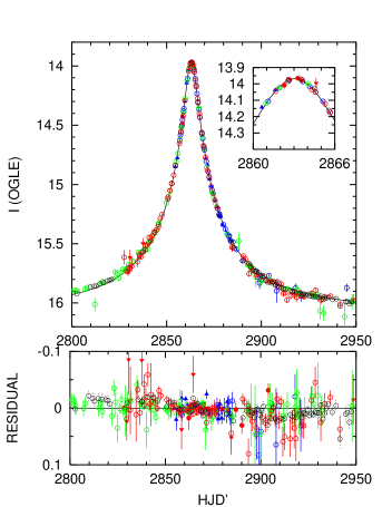
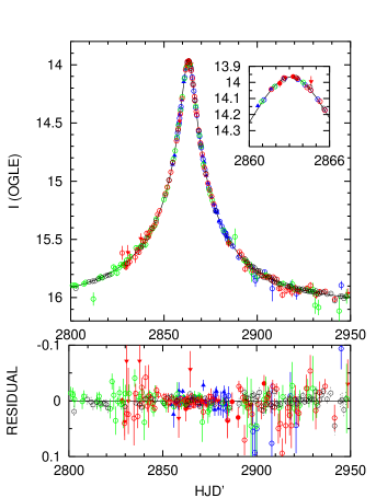
Figure 1: Fit to the lightcurve in the nonparallax (left panel) and the parallax (right panel) models. Data from different collaborations are color-coded as follows: $\mu$FUN, red; MOA, green; OGLE, black; PLANET, blue. Symbols indicate filter bands: $I$, open circles; $V$, inverted triangles; clear, filled circles; $R$, upright triangles. Data have been binned by night. The residuals from the nonparallax fit show an asymmetry about the event peak; the asymmetry disappears when the lightcurve is fit for parallax. The inset shows a zoomed-in view of the peak.

Figure 2: Measurement of the separation of the microlensed source and the unlensed blended light from OGLE astrometry. As described in § 4.1, the blend-source centroid should be at $\boldsymbol{\theta}_{c}[A(t)]=(\boldsymbol{\theta}_{\mathrm{b}}-\boldsymbol{\theta}_{\mathrm{s}})Z(A)+(A\boldsymbol{\mu}_{\mathrm{s}}+r\boldsymbol{\mu}_{\mathrm{b}})W(A,t)+\boldsymbol{\theta}_{0}$ where $r=F_{\mathrm{b}}/F_{\mathrm{s}}$, $W(A,t)=(t-t_{0})/(A+r)$, and $Z(A)=(A_{\rm max}-A)r/[(A_{\rm max}+r)(A+r)]$. The two panels show the residuals, using the best-fit values of $\boldsymbol{\mu}_{\mathrm{s}}$, $\boldsymbol{\mu}_{\mathrm{b}}$ and $\boldsymbol{\theta}_{0}$, in the East and North directions but with the $(\boldsymbol{\theta}_{\mathrm{b}}-\boldsymbol{\theta}_{\mathrm{s}})Z(A)$ term removed. Hence the slopes of the linear fits to these residuals, $(\theta_{\mathrm{b}}-\theta_{\mathrm{s}})_{\rm North}=3.9\pm 7.6\,$mas and $(\theta_{\mathrm{b}}-\theta_{\mathrm{s}})_{\rm East}=-8.5\pm 10.5\,$mas give estimates for the source-blend separation. This separation is consistent with zero within small errors.

Figure 3: Approximately calibrated color-magnitude diagram of stars within a $6^{\prime}$ square of OGLE-2003-BLG-175/MOA-2003-BLG-45. See § 4.2 for details on the calibration procedure. The source (filled circle) lies a magnitude below the center of the bulge clump (triangle) and therefore lies within or behind the bulge. The open circle shows the position of the blend based on $\mu$FUN photometry, and the cross shows the position after the correction based on OGLE photometry. The blended light lies along the “reddening sequence” of foreground disk main-sequence and turnoff stars, which suffer less extinction than the bulge and therefore appear relatively bright and blue in the diagram. Based on this diagram and arguments given in § 4.2, we conclude that the blended light comes from a star of mass $M_{\mathrm{b}}=0.75\,M_{\odot}$ and distance $D_{\mathrm{b}}=1.1\,$kpc.

Figure 4: Left panel: $1\sigma$ contours of the $\chi^{2}$ surfaces, projected onto the $(\pi_{\mathrm{E},E},\pi_{\mathrm{E},N})$ plane, for the $u_{0}>0$ and $u_{0}<0$ fits. The arrow shows the direction of Galactic rotation. The axis ratio of the $u_{0}>0$ “ellipse” is $26:1$ and that of the $u_{0}<0$ one $24:1$. Though only one component of $\boldsymbol{\pi}_{\mathrm{E}}$ is well-constrained, this figure shows that the direction of lens-source relative proper motion is consistent with the direction of Galactic rotation, which supports the hypothesis that the lens is a foreground disk star. The dotted arcs are parts of a circle of radius $\pi_{\mathrm{E}}=0.36$, the predicted microlens parallax. The inset shows the contours with the horizontal scale expanded. Right panel: The solid contours are the same ones shown in the left panel, and are in the geocentric frame. The contours in dashed lines show them transformed to the heliocentric frame.

Figure 5: Expected apparent $I$ magnitude vs. mass, as explained in § 4.2. The observed $I=16.48$ magnitude of the blend is marked with a dotted line. The intersection of the two curves gives our estimate of the mass of the blended light source, $M_{\mathrm{b}}=0.75\,M_{\odot}$.

Figure 6: Even when only one component of the parallax $\boldsymbol{\pi}_{\mathrm{E}}$ is well-determined, it may be possible to constrain the magnitude $\pi_{\mathrm{E}}$ if the source-lens relative proper motion $\boldsymbol{\mu}_{\rm rel}$ is measured. In this figure it is assumed that the $(\pi_{\mathrm{E},\parallel},\pi_{\mathrm{E},\perp})$ axes are rotated from the $(\pi_{\mathrm{E},\mathrm{East}},\pi_{\mathrm{E},\mathrm{North}})$ axes by an angle $\alpha$, that $\pi_{\mathrm{E},\parallel}$ is well-constrained and that $\pi_{\mathrm{E},\perp}$ is not constrained at all. The solid line $l$ is the (very) long axis of the error “ellipse”, which in this case is a strip of width $2\overline{PP^{\prime}}=2\sigma_{\pi_{\mathrm{E},\parallel}}$. The solid line $m$ shows the direction of relative proper motion, and the dotted lines on either side indicate the uncertainty in the direction. The magnitude of $\boldsymbol{\pi}_{\mathrm{E}}$ corresponds to the length of $\overline{OA}$. The uncertainty in the length of $\overline{OA}$ results from the uncertainty $\overline{PP^{\prime}}$ in $\pi_{\mathrm{E},\parallel}$ and the uncertainty $\overline{AA^{\prime}}$ in the direction of $\boldsymbol{\mu}_{\rm rel}$.

Figure 7: Ratio of Einstein timescales $t_{\mathrm{E}}$ in the heliocentric and geocentric frames, evaluated along the contours shown in Figure 4 for the $u_{0}>0$ (solid line) and the $u_{0}<0$ (dashed line) fits. For a given direction of lens-source relative proper motion $\beta=\tan^{-1}(\pi_{\mathrm{E},\mathrm{North}}/\pi_{\mathrm{E},\mathrm{East}})$, ($\beta$ can be inferred from the direction of $\boldsymbol{\mu}_{\rm rel}$) the width of the $1\sigma$ contours corresponds to a variation in $t_{\mathrm{E},\mathrm{hel}}/t_{\mathrm{E},\mathrm{geo}}$ of about 3%.

References

- Alard et al. (1995) Alard, C., Mao, S., & Guibert, J. 1995, A&A, 300, L17
- Albrow et al. (1998) Albrow et al. 1998, ApJ, 509, 687
- Alcock et al. (1993) Alcock et al. 1993, Nature, 365, 621
- Alcock et al. (1995) Alcock, C., et al. 1995, ApJ, 454, L125
- Alcock et al. (1997) Alcock, C., et al. 1997, ApJ, 486, 697
- Alcock et al. (2001) Alcock, C., et al. 2001, Nature, 414, 617
- An et al. (2002) An, J.H., et al. 2002, ApJ, 572, 521
- Aubourg et al. (1993) Aubourg et al. 1993, Nature, 365, 623
- Bennett et al. (2002) Bennett, D.P., et al. 2002, ApJ, 579, 639
- Bond et al. (2001) Bond, I.A. 2001, MNRAS, 327, 868
- Cox (1999) Cox, A.N. 1999, Allen’s Astrophysical Quantities (4th Ed.; New York; Springer)
- Drake et al. (2004) Drake, A. J., Cook, K. H., & Keller, S. C., astro-ph/0404285
- Dyson et al. (1920) Dyson, F.W., Eddington, A.S., & Davidson, C. 1920, Phil. Trans. Roy. Soc., 220A, 291
- Froeschle et al. (1997) Froeschle, M., Mignard, R., & Arenou, F. 1997, Proc. ESA Symp. Hipparcos – Venice ’97 (ESA SP-402, Paris:ESA), 49
- Gaudi & Gould (1997) Gaudi, B. S., & Gould, A. 1997, ApJ, 482, 83
- Gould (1992) Gould, A. 1992, ApJ, 392, 442
- Gould (2000) Gould, A. 2000, ApJ, 542, 785
- Gould (2004) Gould, A. 2004, ApJ, 606, 319
- Gould et al. (2004) Gould, A., Bennett, D. P., & Alves, D. R. 2004, submitted to ApJ (astro-ph/0405124)
- Gould et al. (1994) Gould, A., Miralda-Escudé, J., & Bahcall, J. N. 1994, ApJ, 423, L105
- Gould & Salim (1999) Gould, A., & Salim, S. 1999, ApJ, 524, 794
- Han & Chang (2003) Han, C. & Chang, H-Y. 2003, MNRAS, 338, 637
- Jiang et al. (2004) Jiang, G. et al. 2004, submitted to ApJ
- Mao (1999) Mao, S. 1999, A&A, 350, L19
- Mao et al. (2002) Mao, S., et al. 2002, MNRAS, 329, 349
- Paczyński (1995) Paczyński, B. 1995, Acta Astron., 45, 345
- Paczyński (1986) Paczyński, B. 1986, ApJ, 304, 1
- Park et al. (2004) Park, B.-G. 2004, ApJ, in press (astro-ph/0401250)
- Popowski (2000) Popowski, P. 2000, ApJ, 528, L9
- Refsdal (1964) Refsdal, S. 1964, MNRAS, 128, 295
- Reid (1991) Reid, I.N. 1991, AJ, 102, 1428
- Salim & Gould (2000) Salim, S. & Gould, A. 2000, ApJ, 539, 241
- Smith et al. (2003) Smith, M., Mao, S., & Paczyński, B. 2003, MNRAS 339, 925
- Smith et al. (2003) Smith, M., Mao, S., & Woźniak., P. 2003, ApJ, 585, L65
- Smith et al. (2002) Smith, M., Mao, S., & Woźniak., P. 2002, MNRAS, 332, 962
- Soszyński et al. (2001) Soszyński, I., et al. 2001, ApJ, 552, 731
- Sumi (2004) Sumi, T. 2004, MNRAS, 349, 193
- Udalski et al. (1993) Udalski, A., Szymański, M., Kałużny, J., Kubiak, M., Krzemiński, W., & Mateo, M. 1993, Acta Astron. 43, 69
- Udalski et al. (1994) Udalski, A., Szymański, M., Kałużny, J., Kubiak, M., Mateo, M., Krzemiński, W., & Paczyński, B. 1994, Acta Astron., 44, 227
- Udalski (2003) Udalski, A. 2003, Acta Astron., 53, 291
- Udalski (2003) Udalski, A. 2003, ApJ, 590, 284
- Woźniak (2000) Wozńiak, P.R., Acta Astron., 50, 241
- Yoo et al. (2004) Yoo, J., et al. 2004, ApJ, 603, 139