Dark matter in elliptical galaxies: II. Estimating the mass within the virial radius

Abstract

Elliptical galaxies are modelled with a a 4-component model: Sérsic stars, $\Lambda$CDM dark matter (DM), a $\beta$-model for the hot gas and a central black hole, with the aim of establishing how accurately can one measure the total mass within their virial radii.

DM is negligible in the inner regions, which are dominated by stars and the central black hole. This prevents any kinematical estimate (using a Jeans analysis) of the inner slope of the DM density profile. The gas fraction rises, but the baryon fraction decreases with radius, at least out to 10 effective radii ($R_{e}$). Even with line-of-sight velocity dispersion (VD) measurements at 4 or $5\,R_{e}$ with $20\,\rm km\,s^{-1}$ accuracy and perfectly known velocity anisotropy, the total mass within the virial radius ($r_{v}\equiv r_{200}$) is uncertain by a factor over 3. The DM distributions found in $\Lambda$CDM simulations appear inconsistent with the low VDs measured by Romanowsky et al. (2003) of planetary nebulae between 2 and $5\,R_{e}$, which typically (but not always) imply very low $M/L$s, and a baryon fraction within $r_{v}$ that is greater than the universal value. Replacing the NFW DM model by the new model of Navarro et al. (2004) decreases slightly the VD at a given radius. So, given the observed VD measured at $5\,R_{e}$, the inferred $M/L$ within $r_{v}$ is 40% larger than predicted with the NFW model. Folding in the slight (strong) radial anisotropy found in $\Lambda$CDM (merger) simulations, which is well modelled (much better than with the Osipkov-Merritt formula) with $\beta(r)=1/2\,r/(r+a)$, the inferred $M/L$ within $r_{v}$ is 1.6 (2.4) times higher than for the isotropic NFW model. Thus, the DM model and radial anisotropy can partly explain the low PN VDs, but not in full. The logarithmic slope of the VD at radii of 1 to $5\,R_{e}$, which is insensitive to radius, is another measure of the DM mass within the virial radius, but it is similarly affected by the a priori unknown DM mass profile and stellar velocity anisotropy.

Some of the orbital solutions produced by Romanowsky et al. (2003) indicate that NGC 3379 has a dark matter content at least as large as cosmologically predicted, and the lower $M/L$s of most of their solutions lead to a baryonic fraction within $r_{v}$ that is larger than the universal value. In an appendix, single integral expressions are derived for the VDs in terms of general radial profiles for the tracer density and total mass, for various anisotropic models (general constant anisotropy, radial, Osipkov-Merritt, and the model above).

1 Introduction

Whereas much work has been devoted to constraining the distribution of dark matter in spiral galaxies from a multi-component (disk, bulge, halo, and gas) modelling of their rotation curves (e.g. Persic et al., 1996; Salucci & Burkert, 2000), there have not been analogous analyses for elliptical galaxies, where the components are stars, dark matter, hot gas and the central black hole. Such an analysis is much more difficult for elliptical galaxies, which contrary to spirals, have little rotation (Illingworth, 1977), so that one cannot directly infer the mass profiles from circular velocities (assuming nearly spherical mass distributions).

Instead, one has to analyse the velocity dispersions as a function of position, and this analysis involves solving the Jeans equation, which in spherical symmetry, assuming no streaming motions (including rotation), is

$${{\rm d}(\ell\sigma_{r}^{2})\over{\rm d}r}+2\,{\beta(r)\over r}\,\ell\sigma_{r}^{2}=-\ell(r)\,{GM(r)\over r^{2}}\ ,$$ (1)

where $\ell$ is the luminosity density of the galaxy, $\sigma_{r}$ its radial velocity dispersion, and where the anisotropy parameter is

$$\beta=1-{\sigma_{t}^{2}\over\sigma_{r}^{2}}\ ,$$ (2)

with $\sigma_{t}=\sigma_{\theta}=\sigma_{\phi}$ the 1D tangential velocity dispersion, so that $\beta=0$ corresponds to isotropy, $\beta=1$ is fully radial anisotropy, and $\beta\to-\infty$ is fully tangential anisotropy.

The luminosity density is easily obtained by deprojecting the surface brightness profile, and the situation is simplified by the recent consensus on the applicability to virtually all elliptical galaxies (Caon, Capaccioli, & D’Onofrio, 1993; Bertin, Ciotti, & Del Principe, 2002) of the generalisation (hereafter, Sérsic law) of the $R^{1/4}$ law (de Vaucouleurs, 1948) proposed by Sersic (1968), which can be written as

$$I(R)=I_{0}\exp\left[-\left({R\over a_{S}}\right)^{1/m}\right]\ ,$$ (3)

where $I$ is the surface brightness, $a_{S}$ the Sérsic scale parameter, and $m$ the Sérsic shape parameter, with $m=4$ recovering the $R^{1/4}$ law. Moreover, strong correlations have been reported between the shape parameter $m$ and either luminosity or effective (half projected light) radius $R_{e}$ (Caon et al., 1993; Prugniel & Simien, 1997, and references therein; Graham & Guzmán, 2003).

A serious difficulty in modelling the internal kinematics of elliptical galaxies and clusters of galaxies, considered to be spherical non-rotating systems, is that the Jeans equation (1) has two unknowns: the radial profiles of total mass distribution and velocity anisotropy and this mass / anisotropy degeneracy requires some assumption on anisotropy to recover the total mass distribution. One solution is to analyse the velocity profiles or at least the 4th order velocity moments (Merritt, 1987; Rix & White, 1992; Gerhard, 1993; Łokas & Mamon, 2003; Katgert, Biviano, & Mazure, 2004).

One can go further in modelling the internal kinematics of elliptical galaxies or clusters of galaxies with the Schwarzschild (1979) orbit modelling method, which supposes a form of the potential and minimises the differences between the observations (maps of surface brightness, mean velocity, and velocity dispersion, or even of velocity profiles) and their predictions obtained by suitable projections of linear combinations of a set of orbits that form a basis in energy – angular momentum phase space. One can then iterate over the form of the potential to see if one finds significantly better fits to the observational data. Similarly, Gerhard et al. (1998) suggested working with a set of distribution functions, which one hopes forms an adequate basis, and one then minimises the linear combination of the distribution functions that match best the observations. However, such recent analyses rarely place useful constraints on the gravitational potential (with no priors), with the exception of Kronawitter et al. (2000), who find that some elliptical galaxies are consistent with constant mass-to-light ratios while others show mass rising faster than light.

The key issue is to obtain more distant tracers of the gravitational potential. Two such studies, by Méndez et al. (2001) and Romanowsky et al. (2003), of the distribution of the line-of-sight velocities of planetary nebulae (hereafter, PNe) on the outskirts of a total of four moderately luminous ($L_{*}$) nearby elliptical galaxies indicate fairly rapidly decreasing PN velocity dispersion profiles. Romanowsky et al. carefully analyse one of their galaxies (NGC 3379) with the Schwarzschild method, and their favourite conclusion is that the dark matter content of these galaxies is low at 5 effective radii, and extrapolates to a very low mass-to-blue-light ratio of $\Upsilon_{B}=33$ at 120 kpc, which they consider as the virial radius. This low mass-to-light ratio at the virial radius (hereafter, virial mass-to-light ratio) appears to be at strong variance with the cosmological predictions: Two recent works suggest that $\Upsilon_{B}$ has a non-monotonic variation with mass (or luminosity), with a minimum value around 80–100 for luminosities $L_{B}\approx 10^{9-11}\,{\rm L_{\odot}}$ (Marinoni & Hudson, 2002; Yang et al., 2003), both studies predicting $\Upsilon_{B}\simeq 100\,h_{70}$ for $L_{B}=L_{B,*}=1.88\times 10^{10}L_{\odot}$ (Mamon & Łokas, 2005).

There are various alternatives to estimating the mass profiles of elliptical galaxies through the Jeans equations, in particular modelling the X-ray emission arising from hot gas assumed in hydrostatic equilibrium in the gravitational potential, through the effects of gravitational lensing and through the kinematic analysis of galaxy satellites.

The analyses of diffuse X-ray emission in elliptical galaxies have the advantage that the equation of hydrostatic equilibrium, which is the gas equivalent of the Jeans equation (1), has no anisotropy term within it, so in spherical symmetry, one can easily derive the total mass distribution. However, the derivation of the total mass profile requires measuring the temperature profile and its gradient, and unfortunately, even with the two new generation X-ray telescopes XMM-Newton and Chandra, it is difficult to achieve such measurements beyond half the virial radius for galaxy clusters (Pointecouteau et al., 2005; Vikhlinin et al., 2005), and even much less for elliptical galaxies. Moreover, the X-ray emission from elliptical galaxies is the combination of two components: diffuse hot gas swimming in the gravitational potential as well as direct emission from individual stars, and it is highly difficult to disentangle the two (see Brown & Bregman, 2001). Assuming that all the X-ray emission is due to the diffuse hot gas, Loewenstein & White (1999) provide interesting constraints on the dark matter in luminous ($L>L_{*}$) ellipticals, with a dark matter mass fraction of $\mathrel{\hbox{\hbox to0.0pt{\hbox{\lower 4.0pt\hbox{$\sim$}}\hss}\hbox{$>$}}}20\%$ (39%) at $R=R_{e}$ ($5\,R_{e}$).

Weak gravitational lensing is yet another avenue to analyse the gravitational potential of elliptical galaxies. Since the signal is much too weak for individual galaxies, one has to stack thousands of galaxies together. In this manner, Wilson et al. (2001) find that the gravitational lensing shear falls off with angular distance as expected for a structure whose circular velocity is roughly independent of radius, which suggests appreciable amounts of dark matter at large radii. Moreover, from their analysis of SDSS galaxies, Guzik & Seljak (2002) find that $L_{*}$ galaxies have mass-to-light ratio $\Upsilon$ of order of 100 in the $B$ band, again implying substantial dark matter, since the stellar contribution to the mass-to-light ratio is thought to be only $\Upsilon_{*}\simeq 8$ in the blue band (see e.g. Gerhard et al., 2001). Recently, Hoekstra, Yee, & Gladders (2004) derived from the gravitational lensing shear profile of RCS galaxies, a Navarro, Frenk, & White (hereafter, NFW) mass within the virial radius, corresponding to $\Upsilon_{B}\simeq 59\pm 5$.

The constraints from the internal kinematics of galaxy satellites, pioneered by Zaritsky & White (1994), are now showing consistency with the $\Lambda$CDM models (Prada et al., 2003). However, one needs to stack the data from many galaxies, so errors in stacking can accumulate, and the method is very sensitive to the correct removal of interlopers (Prada et al.).

The constraints on the dark matter are greatly strengthened when combining the internal kinematics with either the X-ray or gravitational lensing approach. Combining internal kinematics with X-rays, Loewenstein & White (1999) are able to constrain the dark matter contents of ellipticals, although they make use of the not very realistic Osipkov-Merritt (Osipkov, 1979; Merritt, 1985) anisotropy (see Fig. 2 below). Combining internal kinematics with the constraints from strong gravitational lensing, Treu & Koopmans (2002, 2004) are able to constrain the slope of the inner density profile of the dark matter.

On the theoretical side, large-scale dissipationless cosmological $N$-body simulations have recently reached enough mass and spatial resolution that there appears to be a convergence on the structure and internal kinematics of the bound structures, usually referred to as halos, in the simulations. In particular, the density profiles have an outer slope of $\simeq-3$ and an inner slope between $-1$ (Navarro, Frenk, & White, 1995, 1996) and $-3/2$ (Fukushige & Makino, 1997; Moore et al., 1999; Ghigna et al., 2000). In this paper, we consider the general formula that Jing & Suto (2000) found to provide a good fit to simulated halos:

$$\rho(r)\propto\left({r\over a_{d}}\right)^{-\alpha}\,\left[1+\left({r\over a_{d}}\right)\right]^{\alpha-3}\ ,$$ (4)

where the absolute value of the inner slope $\alpha=1$ or 3/2, and ‘$d$’ stands for dark. These profiles fit well the density profiles of cosmological simulations out to the virial radius $r_{v}$, wherein the mean density is $\Delta\approx 200$ times the critical density of the Universe, and are characterized by their concentration parameter

$$c={r_{v}\over a_{d}}\ .$$ (5)

Recently, a number of numerical studies have proposed better analytic fits to the radial profiles of density (Diemand et al., 2004a), density logarithmic slope (Navarro et al., 2004) or circular velocity (Stoehr et al., 2002; Stoehr, 2006) profiles of simulated halos. In particular, the formula of Navarro et al. is attractive because it converges to a finite central density at very small scales and has an increasing outer slope with a finite mass. Moreover, fitting to the logarithmic slope of the density profile is to be preferred on the grounds that fitting the density or circular velocity involves fitting a single or double integral of the density slope, thus possibly missing details smoothed over in the integrals. We shall therefore focus on the density profile of Navarro et al. (hereafter, Nav04) in this work.

Two recent studies have placed interesting constraints on the dark matter distribution within elliptical galaxies. Borriello, Salucci, & Danese (2003) compute the aperture velocity dispersions of models with an NFW dark matter component and a Sérsic luminosity component. They find that the dark matter content must be either low or with a concentration parameter roughly 3 times lower than fit in the dissipationless cosmological $N$-body simulations, for otherwise the fundamental plane of elliptical galaxies is curved more than allowed by observations. Napolitano et al. (2005) estimate the mass-to-light ratio gradient for a large number of observed ellipticals. They find that very luminous ellipticals appear to have large $M/L$ gradients consistent with important quantities of dark matter within the virial radius, while the lower luminosity $L\mathrel{\hbox{\hbox to0.0pt{\hbox{\lower 4.0pt\hbox{$\sim$}}\hss}\hbox{$<$}}}L_{*}$ ellipticals appear to have very low gradients, that can be explained either by a strong lack of dark matter, or else by a dark matter concentration parameter much lower ($c\simeq 1-6$) than expected from cosmological $N$-body simulations ($c\simeq 15$). It remains to be seen how dependent are the conclusions of Napolitano et al. on the kinematical modelling of their ellipticals.

Our basic goal is to place constraints on the total mass distribution of elliptical galaxies. In a companion paper (Mamon & Łokas, 2005, hereafter, paper I), we show that the NFW, Jing & Suto (hereafter, JS–1.5), and Nav04 density profiles found in dissipationless cosmological simulations cannot represent the total matter distribution in elliptical galaxies, because: 1) the local mass-to-light ratios are then far below the generally admitted values for the stellar component; and 2) the aperture and slit-averaged velocity dispersions are much lower than observed for their luminosities (i.e. through the Faber & Jackson, 1976 relation). We also show that the highly concentrated NFW models that X-ray observers have fit to the total mass density profile of ellipticals are an artifact of fitting to the combination of a Sérsic stellar component and an NFW dark matter component, and that the fits cannot be very good. Finally, we argue that the very low local mass-to-light ratios and aperture velocity dispersions found imply that the stellar component fully dominates the internal kinematics of the inner few effective radii, suggesting that there is little hope in recovering the inner slope of the dark matter density profile. All these conclusions suppose that the total mass density profile inside an effective radius does not sharply steepen to a slope of order $-2$ or steeper.

In the present paper, making no direct assumptions on the total mass density profile, we focus on the velocity dispersions and mass profiles in the outer parts of elliptical galaxies, from 1 to 5 effective radii. For this, we build a detailed 4-component model of elliptical galaxies, with stars, dark matter, hot diffuse gas and a central black hole (as we don’t know, a priori, whether these last two components affect the kinematical analysis of dark matter in ellipticals). It is very possible that the dark matter reacts to the presence of the baryon component, which can be treated by the approximation of adiabatic contraction, and recent simulations with gas suggest that the resulting dark matter density profile scales as $1/r^{2}$ over a wide range of radii (Gnedin et al., 2004 using cosmological simulations, and Dekel et al., 2005 using galaxy merging simulations). Whereas such an “isothermal” distribution is a real possibility for the dark matter, it remains unclear how feedback processes from the baryons (as modelled by Cox et al., 2005 for the results given by Dekel et al.) may affect this result. We therefore assume here, as in paper I, that the dark matter distribution follows the more robust predictions from dissipationless $\Lambda$CDM cosmological $N$-body simulations.

The plan of our paper in as follows: In Sec. 2, we describe our 4-component model, in Sec. 3.1, we consider the mass-to-light ratios consistent with the orbit modelling of Romanowsky et al. (2003) on the stellar and PN kinematics in NGC 3379, and in Sec. 3.2, we estimate the velocity anisotropy of the particles in dissipationless cosmological $N$-body simulations. We study the effects of velocity anisotropy in Sec. 4.1, compare the importance of the different components in Sec. 4.2, and ask whether we can weigh the dark matter component in Sec. 4.3. We discuss our results in Sect. 5, and reflect on the very low mass-to-light ratio reported by Romanowsky et al. (2003) for intermediate luminosity elliptical galaxies. In Appendix A, we derive single quadrature expressions for the radial profiles of the line of sight velocity dispersion in terms of general tracer density and total mass profiles for four simple anisotropy models.

2 Basic equations

We now highlight the 4-component model that we adopt for elliptical galaxies: stars, diffuse dark matter, hot gas, and a central black hole. We neglect any contribution from dark baryons (e.g. MACHOs).

2.1 Distribution of optical light

We begin with the distribution of optical light, referring the reader to paper I for details. The Sérsic (eq. [3], see detailed properties in Graham & Driver, 2005) optical surface brightness profile that represents the projected stellar distribution, can be deprojected according to the approximation first proposed by Prugniel & Simien (1997)

$$\ell(r) = \ell_{1}\,\widetilde{\ell}(r/a_{S})$$ (6)

$$\widetilde{\ell}(x) \simeq x^{-p}\,\exp\left(-x^{1/m}\right)\ ,$$ (7)

$$\ell_{1} = \left\{{\Gamma(2m)\over\Gamma[(3-p)\,m]}\right\}\,{I_{0}\over 2\,a_{S}}\ ,$$ (8)

$$p \simeq 1.0-0.6097/m+0.05463/m^{2}\ ,$$ (9)

where the last equation is from Lima Neto et al. (1999).

The integrated luminosity corresponding to equations (6), (7) and (8) is then (Lima Neto et al.)

$$L_{3}(r) = L\,\widetilde{L}_{3}(r/a_{S})$$ (10)

$$\widetilde{L}_{3}(x) = {\gamma\left[(3-p)m,x^{1/m}\right]\over\Gamma[(3-p)m]}\ ,$$ (11)

where the total luminosity of the galaxy is

$$L=2\pi m\,\Gamma(2m)\,I_{0}\,a_{S}^{2}=4\pi m\,\Gamma\left[(3-p)\,m\right]\,\ell_{1}\,a_{S}^{3}\ ,$$ (12)

as obtained by Young & Currie (1994) from the Sérsic surface brightness profile of equation (3), and which matches exactly the total luminosity obtained by integration of Lima Neto et al.’s approximate deprojected profile.

It is useful to express radii in terms of the effective radius, $R_{e}$, which is the radius of half projected light, where

$$R_{e} = b^{m}\,a_{S}$$ (13)

$$b \simeq 2\,m-1/3+0.009876/m\ ,$$ (14)

where the latter relation is from Prugniel & Simien (1997). In paper I, we showed that $R_{e}$ and $m$ are fairly well correlated with total luminosity:

$$\log h_{70}\,R_{e}^{\rm(fit)} \!\!\!\!=\!\!\!\! 0.34+0.54\,\log L_{10}+0.25\,\left(\log L_{10}\right)^{2}\ ,$$ (15)

$$\log m^{\rm(fit)} \!\!\!\!=\!\!\!\! 0.43+0.26\,\log L_{10}-0.044\,\left(\log L_{10}\right)^{2}\,,$$ (16)

where $L_{10}=h_{70}^{2}\,L_{B}/\left(10^{10}{\rm L_{\odot}}\right)$, $R_{e}^{\rm(fit)}$ is measured in kpc, and with $H_{0}=100\,h=70\,h_{70}\,\rm km\,s^{-1}\,Mpc^{-1}$. Then, equations (13) and (14) lead to

$$a_{S}\simeq\left[b\left(m^{\rm(fit)}\right)\right]^{-m^{\rm(fit)}}R_{e}^{\rm(fit)}\ .$$ (17)

2.2 The central black hole

High spatial resolution spectroscopic studies of ellipticals have shown that they almost always harbour a supermassive black hole of mass 0.2% (Faber et al., 1997), 0.3% (Kormendy et al., 1997), or 0.6% (Magorrian et al., 1998) that of the stellar component. We thus define the fraction of black hole mass to stellar mass

$$g_{\rm BH}={M_{\rm BH}\over\Upsilon_{*}\,L_{3}(r_{v})}\ .$$ (18)

We could have defined $g_{\rm BH}$ in terms of the total luminosity instead of that at the virial radius, but the two differ by typically less than 0.1%, which is much less than the uncertainty on $g_{\rm BH}$, and the latter scaling generates simpler equations below. A recent analysis (Häring & Rix, 2004) favours $g_{\rm BH}=0.15\%\,\left(M_{\rm bulge}/6\times 10^{11}{\rm M_{\odot}}\right)^{0.12}$, and we will adopt below $g_{\rm BH}=0.15\%$. The precise value of $g_{\rm BH}$ has a negligible effect on the constraints on dark matter in elliptical galaxies.

2.3 Scalings of global properties

We adopt a fiducial luminosity of $L=L_{*}$. In paper I, we derived, from Liske et al. (2003), a blue-band luminosity $L_{*,B}=1.88\,10^{10}\,h_{70}^{-2}{\rm L_{\odot}}$, i.e. an absolute magnitude of $M_{B}=-20.24$, using (e.g., Colina et al., 1996)

$$M_{B}^{\odot}=5.45\ .$$ (19)

Our choice of $L_{B}$ translates to $m=3.15$ (eq. [16]), $R_{e}=3.2\,\,h_{70}^{-1}\,\rm kpc$ (eq. [15]) and $a_{S}=11.6\,h_{70}^{-1}\rm pc$ (eq. [17]).

In paper I, we argued that the blue stellar mass-to-light ratios of elliptical galaxies lay in the rough range from 5 to 8, where the uncertainty is caused by the uncertain initial mass function and its lower and upper mass cutoffs, as well as metallicity and stellar evolution code. In the present paper, we adopt the mean: $\Upsilon_{*,B}=6.5$, unless specified otherwise.

We also showed in paper I that the mass-to-light ratio of the Universe is

$$\overline{\Upsilon}_{B}=\Omega_{m}\,\Upsilon_{{\rm closure},B}={3\,\Omega_{m}H_{0}^{2}\over 8\pi\,G\,j_{B}}=390\,h_{70}\ ,$$ (20)

given the luminosity density found by Liske et al. (2003) and Blanton et al. (2003) in the 2dFGRS and SDSS surveys, respectively.

We define the mass-to-light ratio bias

$$b_{\Upsilon}={\Upsilon\over\overline{\Upsilon}}\ ,$$ (21)

where $\Upsilon=M_{t}/L(r_{v})$, with $M_{t}$ the total mass within the virial radius. If the Universe is unbiased, i.e. the mass-to-light ratio within the virial radius will be $\Upsilon_{B}=\overline{\Upsilon}_{B}=390\,h_{70}$. The internal kinematics of galaxy clusters are consistent with the universal mass-to-light ratio (e.g. Łokas & Mamon, 2003 derive $\Upsilon_{B}=351$ for the Coma cluster). Following the predictions of Marinoni & Hudson (2002) and Yang et al. (2003), we will adopt a standard value $\Upsilon_{B}=\Upsilon_{B}^{\rm std}=100\,h_{70}$.

We also define the baryon fraction bias

$$b_{b}={f_{b}\over\overline{f}_{b}}={f_{b}\over\left(\Omega_{b}/\Omega_{m}\right)}\ ,$$ (22)

where $f_{b}$ is the baryon fraction within the virial radius, while $\overline{f}_{b}=\Omega_{b}/\Omega_{m}\simeq 0.14$ is the mean baryon fraction of the Universe. We used here the big-bang nucleosynthesis measurement $\Omega_{b}=0.02\,h^{-2}=0.041$ (O’Meara et al., 2001), which is consistent with the value obtained by Spergel et al. (2003) from the WMAP CMB experiment, and $\Omega_{m}=0.3$.

Given the fractions of mass in stars, the central black hole, hot gas and dark matter, all at the virial radius:

$$f_{*} = {\Upsilon_{*}\over b_{\Upsilon}\,\overline{\Upsilon}}\ ,$$ (23)

$$f_{\rm BH} = g_{\rm BH}\,f_{*}\ ,$$ (24)

$$f_{d} = 1-f_{b}=1-b_{b}\,\overline{f}_{b}\ ,$$ (25)

$$f_{g} = 1-\left(f_{*}+f_{\rm BH}+f_{d}\right)\ ,$$ (26)

where we assumed that the central black hole originates from baryons (this assumption has a negligible effect on what follows), it is easy to show that these two biases are related through

$$b_{b}\,b_{\Upsilon}={1\!+g\!+\!g_{\rm BH}\over\overline{f}_{b}}\,\left({\Upsilon_{*}\over\overline{\Upsilon}}\right)\simeq{1\!+\!g\over\overline{f}_{b}}\,\left({\Upsilon_{*}\over\overline{\Upsilon}}\right)\ ,$$ (27)

where $g$ is the gas to star ratio within the virial radius, and $\Upsilon_{*}$ is the mass-to-light ratio of the stellar population, assumed independent of radius (in conformance with the very weak colour gradients in ellipticals, e.g. Goudfrooij et al., 1994).

If mass is biased relative to luminosity in elliptical galaxies ($b_{\Upsilon}\neq 1$), we can assume that the baryon fraction is unaffected ($b_{b}=1$, and $g$ must vary according to eq. [27]). Indeed, it is difficult to conceive of a mechanism that will segregate baryons from dark matter within a radius as large as the virial radius. For the gas to star ratio to be positive, one then requires

$$\Upsilon_{B}>{\Upsilon_{*,B}\over\overline{f}_{b}}=48\,\left({\Upsilon_{*,B}\over 6.5}\right)\ .$$ (28)

In other words, considering more mass in stars requires a larger minimum total mass at the virial radius for the baryon fraction to retain its universal value. Turning the argument around, a low total mass-to-light ratio at the virial radius would imply that the baryonic fraction is greater than the universal value, i.e. $b_{b}>1$. Indeed, the general equation (27) implies

$$b_{b}>{\Upsilon_{*}/\Upsilon\over\overline{f}_{b}}=1.0\ {\Upsilon_{*}/6.5\over\Upsilon/48}\ ,$$ (29)

where the equality is for a negligible gas-to-star ratio $g$.

2.4 Distribution of dark mass

We consider here three dark matter models: the NFW model with inner slope $-1$, the generalized NFW model introduced by Jing & Suto (2000) with inner slope $-3/2$ (JS–1.5), and the convergent model of Navarro et al. (2004, Nav04). The dark matter density profile can generally be written (see paper I, especially for the Nav04 model):

$$\rho_{d}(r) \!\!\!\!=\!\!\!\! {c^{3}\over g_{d}(c)}\,\left({M_{d}\over 4\pi\,r_{v}^{3}}\right)\,\widetilde{\rho}_{d}(r/a_{d})\ ,$$ (30)

$$\widetilde{\rho}_{d}(y) \!\!\!\!=\!\!\!\! \left\{\!\!\begin{array}[]{lll}y^{-\alpha}\,(1+y)^{\alpha-3}&\!\!\!\!\alpha=1\ \hbox{(NFW)},\ \alpha=3/2\ \hbox{(JS--1.5)}\ ,\\ &\\ \exp\left(-{2\mu}\,y^{1/\mu}\right)&\hbox{(Nav04)}\ ,\end{array}\right.$$ (34)

$$g_{d}(y) \!\!\!\!=\!\!\!\! \left\{\!\!\!\!\begin{array}[]{ll}\ln(y+1)-y/(y+1)&\!\!\!\!\hbox{(NFW)}\ ,\\ &\\ 2\,\left[\sinh^{-1}\sqrt{y}-\sqrt{y/(y\!+\!1)}\right]&\!\!\!\!\hbox{(JS--1.5)}\ ,\\ &\\ {1\over 2}\,\left(2\,\mu\right)^{1-3\,\mu}\,\gamma\left[{3\,\mu},{2\,\mu}\,y^{1/\mu}\right]&\!\!\!\!\hbox{(Nav04)}\ ,\end{array}\right.$$ (40)

where $\alpha$ is the absolute value of the logarithmic slope of the inner density profile (for the NFW and JS–1.5 models), $c$ is the concentration parameter (eq. [5]), $a_{d}$ is the radius where the logarithmic slope is equal to $-2$ (NFW, Nav04) or $-9/4$ (JS–1.5, for which $a_{d}/2$ is the radius where the slope is $-2$), $\mu\simeq 6$ (paper I), and $\sinh^{-1}x=\ln(x+\sqrt{x^{2}+1})$ for $x>0$. In equation (30), $M_{d}$ is the dark mass within the virial radius, defined such that the mean total density within it is $\Delta=200$ times the critical density of the Universe, $\rho_{\rm crit}=3\,H_{0}^{2}/(8\,\pi G)$, yielding a virial radius (see Navarro et al., 1997)

$$r_{v} = \left({2\,G\,M_{v}\over\Delta\,H_{0}^{2}}\right)^{1/3}\ ,$$ (41)

$$= 163\,h^{-1}\,{\rm kpc}\,\left({h\,M_{t}\over 10^{12}\,{\rm M_{\odot}}}\right)^{1/3}\ ,$$

$$= 206\,h_{70}^{-1}\,{\rm kpc}\,\left({h_{70}M_{t}\over 10^{12}\,{\rm M_{\odot}}}\right)^{1/3}\ ,$$

for $\Delta=200$. Jing & Suto (2000) measured the concentration parameter $c$ (eq. [5]) from their $\Lambda$CDM (with cosmological density parameter $\Omega_{m}=0.3$ and dimensionless cosmological constant $\Omega_{\Lambda}=0.7$) simulations, which can be fit by the relations

$$c\simeq\left\{\begin{array}[]{ll}\displaystyle 10.2\,M_{12}^{-0.08}&(\hbox{NFW})\ ,\\ &\\ \displaystyle 4.9\,M_{12}^{-0.13}&(\hbox{JS--1.5})\ ,\end{array}\right.$$ (42)

where $M_{12}={hM_{t}/10^{12}{\rm M_{\odot}}}$. In paper I, we derived the concentration parameter of the Nav04 model:

$$c=8.1\,M_{12}^{-0.11-0.015\,\log M_{12}}\,$$ (43)

which is similar to the concentration parameters in equations (42). For $L_{B}=L_{*,B}$, equations (15) and (41) lead to

$${r_{v}\over R_{e}}=79\,\left({\Upsilon_{B}\over 100}\right)^{1/3}\ .$$ (44)

The cumulative mass of the dark models used here can all be written

$$M_{d}(r) = M_{d}\,\widetilde{M}_{d}(r/a_{d})\ ,$$ (45)

$$\widetilde{M}_{d}(y) = {g_{d}(y)\over g_{d}(c)}\ ,$$ (46)

where $g_{d}(y)$ is given in equation (40).

A complication arises because the luminosity at the virial radius is very close to but not exactly equal to the total luminosity. We write out the total mass at the virial radius, both as a mean density threshold, and as the luminosity at the virial radius times the mass-to-light ratio:

$$M_{t}={4\pi\over 3}\,r_{v}^{3}\,\Delta\,\rho_{\rm crit}={\Delta H_{0}^{2}r_{v}^{3}\over 2\,G}=\Upsilon\,L\,\widetilde{L}_{3}(r_{v}/a_{s})\ ,$$ (47)

(where we used eq. [21]) and solve the last equality of equation (47) for $r_{v}$ (the correction on $r_{v}$ turns out to be negligible as the luminosity has nearly fully converged at the virial radius).

2.5 Distribution of gas mass

Elliptical galaxies also shine X-rays. Both discrete sources and a hot diffuse interstellar medium contribute to their X-ray emission, and the latter component should contribute non-negligibly to the mass budget of ellipticals. Indeed, if elliptical galaxies are unbiased matter tracers ($b_{\Upsilon}=1$), then according to equation (23), stars contribute at the virial radius to a fraction of the total mass of $f_{*}=\Upsilon_{*}/\overline{\Upsilon}=0.017\,(\Upsilon_{*}/6.5)$. This is much less than the baryon fraction at the virial radius assuming no baryon bias ($b_{b}=1$), i.e. $f_{b}=\overline{f}_{b}=0.14\,h_{70}^{-2}$ (Sect. 2.3). So, if ellipticals have the same baryon fraction within their virial radius as the full Universe, then the hot gas in ellipticals accounts for $0.14\,h_{70}^{-2}-0.025\,h_{70}^{-1}=0.11$ (for $h_{70}=1$) of the total mass within the virial radius (assuming no dark baryons), which is $0.11/0.025\simeq 4$ times more than stars. If elliptical galaxies have virial mass-to-light ratios as low as $\Upsilon_{B}=100$, then the gas-to-star ratio is lower (for fixed baryonic fraction). According to equation (27), for no baryon bias ($b_{b}=1$), the gas dominates the stars at the virial radius ($g>1$) for $\Upsilon_{B}>2\Upsilon_{*,B}/\overline{f}_{b}=93\left(\Upsilon_{*,B}/8\right)$.

Brown & Bregman (2001) have fit the X-ray surface brightness profiles of luminous ellipticals (jointly with a component for discrete sources following the $R^{1/4}$ law), and find that the usual so called $\beta$-model

$$\rho_{g}(r) = \rho_{0}\,\widetilde{\rho}_{g}(r/r_{c})$$ (48)

$$\widetilde{\rho}_{g}(z) = \left(1+z^{2}\right)^{-3\beta_{g}/2}\ ,$$ (49)

provides a good representation of the distribution of the hot gas, with $\langle\beta_{g}\rangle=0.49$ and

$$r_{c}\simeq{R_{e}\over q}\ ,$$ (50)

where $q\simeq 10$. Using a larger sample of elliptical galaxies, O’Sullivan et al. (2003) find a mean $\beta_{g}$ of 0.55, but do not estimate $r_{c}/R_{e}$. These parameters should be considered tentative, as the subtraction of the hard stellar component is quite uncertain.

As for the other non-stellar components, the gas enters our analysis only through its cumulative mass (see the Jeans equation [1]). Adopting

$$\beta_{g}=1/2\ ,$$ (51)

the cumulative mass distribution arising from equation (48) is,

$$M_{g}(r) \!\!\!\!=\!\!\!\! {4\,\pi}\,\rho_{0}\,r_{c}^{3}\,\widetilde{M}_{g}(r/r_{c})$$ (52)

$$\widetilde{M}_{g}(z) \!\!\!\!=\!\!\!\! {2\over 3}\,z\,\left[(1+z^{2})^{1/4}-{}_{2}F_{1}\left({1\over 2},{3\over 4};{3\over 2};-z^{2}\right)\right]\ ,$$ (53)

where ${}_{2}F_{1}(a,b;c;x)=\Gamma(c)/[\Gamma(b)\Gamma(1\!-\!b)]\int_{0}^{1}t^{b\!-\!1}(1\!-\!t)^{c\!-\!b\!-\!1}(1\!-\!tx)^{-a}$ is a the Hypergeometric function. Note that $\widetilde{M}_{g}(1)\simeq 0.239$.

To an accuracy of 2.7% for all $z$, one has

$$\widetilde{M}_{g}(z)\simeq\left[\left({1\over 3}\,z^{3}\right)^{-\gamma}+\left({2\over 3}\,z^{3/2}\right)^{-\gamma}\right]^{-1/\gamma}\ ,$$ (54)

with $\gamma=2^{1/8}\simeq 1.0905$.

We write the gas mass profile as

$$M_{g}(r)=M_{g}(r_{v})\,{\widetilde{M}_{g}(r/r_{c})\over\widetilde{M}_{g}(r_{v}/r_{c})}$$ (55)

and normalise the gas component with the baryon fraction within the virial radius:

$${M_{g}(r_{v})\over M_{t}}=f_{b}-\left(1+g_{\rm BH}\right)\,f_{*}=b_{b}\,\overline{f}_{b}-\left(1+g_{\rm BH}\right)\,{\Upsilon_{*}\over\Upsilon}\ .$$ (56)

The divergence of the gas mass profile at large radii is very severe ($M_{g}\propto r^{3/2}$), leading to a divergent gravitational potential, and to a local gas fraction much too large. We therefore assume that, beyond the virial radius, the ratio of local baryon (gas + stellar) mass density to local total matter density is equal to the universal baryon ratio $\overline{f}_{b}=\Omega_{b}/\Omega_{m}$, yielding

$$\rho_{g}(r)={\overline{f}_{b}\over 1-\overline{f}_{b}}\,\rho_{d}(r)-\Upsilon_{*}\,\ell(r)\qquad\hbox{ for }r>r_{v}\ ,$$ (57)

where $\rho_{d}$ is the dark matter density.

The local gas density profile will therefore be discontinuous at the virial radius. Physically, one expects a shock to occur at the interface between the gas infalling into the galaxy and the gas in equilibrium within the galaxy, and this shock should occur very close to the virial radius. With equations (48), (49), (50), (51), (52), (54), and (56), the local gas density profile just within the virial radius is (dropping the negligible $1+g_{\rm BH}$ term in eq. [56])

$$\rho_{g}(r_{v}^{-})=\left(b_{b}\,\overline{f}_{b}-{\Upsilon_{*}\over\Upsilon}\right){\left(1+r_{v}^{2}/r_{c}^{2}\right)^{-3/4}\over\widetilde{M}_{g}(r_{v}/r_{c})}\,\left({M_{t}\over 4\pi r_{c}^{3}}\right)\,,$$ (58)

while with equations (30), (34), (40), and (57), the local gas density just outside the virial radius is

$$\rho_{g}(r_{v}^{+}) \!\!\!\!=\!\!\!\! \left\{{\left[c/(c+1)\right]^{3-\alpha}\over g_{d}(c)}\,\overline{f}_{b}\left({1-b_{b}\,\overline{f}_{b}\over 1-\overline{f}_{b}}\right)\,\right.$$ (59)

$$\left.-{(r_{v}/a_{S})^{3}\,\widetilde{\ell}(r_{v}/a_{S})\over m\,\Gamma[(3-p)m]\,\widetilde{L}_{3}(r_{v}/a_{S})}\,{\Upsilon_{*}\over\Upsilon}\right\}\,\left({M_{t}\over 4\pi r_{c}^{3}}\right)\,.$$

According to equations (58) and (59), the discontinuity of the gas density at the virial radius can be written

$${\rho_{g}(r_{v}^{+})\over\rho_{g}(r_{v}^{-})} = {1\over b_{b}\Upsilon\,\overline{f}_{b}-\Upsilon_{*}}\,{\left(1+z_{v}^{2}\right)^{3/4}\,\widetilde{M}_{g}(z_{v})\over z_{v}^{3}}$$ (60)

$$\times\left\{\Upsilon\,\overline{f}_{b}\,\left({1-b_{b}\,\overline{f}_{b}\over 1-\overline{f}_{b}}\right)\,\,{\left[c/(c+1)\right]^{3-\alpha}\over g_{d}(c)}\right.$$

$$\qquad-\left.{\Upsilon_{*}\over m\Gamma[(3-p)m]}\,{x_{v}^{3}\,\widetilde{\ell}(x_{v})\over\widetilde{L}_{3}(x_{v})}\right\}\ ,$$

where $x_{v}={r_{v}/a_{S}}$ and $z_{v}=r_{v}/r_{c}$. For a wide variety of plausible parameters $\Upsilon_{*}$, $b_{b}$, $\Upsilon$, $\alpha$, $c$, $x_{v}$ and $z_{v}$, equation (60) yields density ratios $\rho_{g}(r_{v}^{-})/\rho_{g}(r_{v}^{+})$ between 2 and 3.5, in accordance with the standard Rankine-Hugoniot conditions (density ratio smaller than 4).

The cumulative gas mass beyond the virial radius is then

$$M_{g}(r) = M_{g}(r_{v})+{\overline{f}_{b}\over 1-\overline{f}_{b}}\,\left[M_{d}(r)-M_{d}(r_{v})\right]$$ (61)

$$\qquad\ \ \ \ \,-\Upsilon_{*}\,\left[L(r)-L(r_{v})\right]\ ,$$

yielding a normalized gas mass satisfying

$${\widetilde{M}_{g}(z)\over\widetilde{M}_{g}(z_{v})}-1 = {M_{g}(r)\over M_{g}(r_{v})}-1$$ (62)

$$= {f_{d}\over f_{g}}\,{\overline{f}_{b}\over\left(1\!-\!\overline{f}_{b}\right)}\,\left[\widetilde{M}_{d}\left({r\over a_{d}}\right)-1\right]$$

$$\quad-{f_{*}\over f_{g}}\,\left[{\widetilde{L}_{3}\left(r/a_{S}\right)\over\widetilde{L}_{3}\left(r_{v}/a_{S}\right)}-1\right]\ ,$$

where the second term is negligible (as the integrated luminosity has almost fully converged at the virial radius).

3 Other astronomical inputs

3.1 Lower bound on the virial mass-to-light ratio

Our lower bound on the mass-to-light ratio within the virial radius is taken from the work of Romanowsky et al. (2003), who performed, for the nearby giant elliptical, NGC 3379, an orbit modelling of the velocity field of the planetary nebulae combined with the radial profiles of the stellar surface brightness and line-of-sight velocity dispersion. Although they quote a mass-to-light ratio at 120 kpc, which they estimate as the virial radius, of $\Upsilon_{B}=33\pm 14$, we find

$$\Delta(r)=2\,{\Upsilon_{B}\,G\,L_{B}\over H_{0}^{2}\,r^{3}}=507\ ,$$ (63)

for $r=120\,\rm kpc$, $\Upsilon_{B}=33$, and $L_{B}=1.51\times 10^{10}\,L_{\odot}$ (from Romanowsky et al.’s $M_{B}=-20.0$ and eq. [19]). So clearly the radius of overdensity 200 is much larger than 120 kpc, and since dark matter is believed to be more extended than luminous matter (e.g., Fig. 4), the mass-to-light ratio should be larger than 33.

We extrapolate Romanowsky et al.’s mass-to-light ratio out to the virial radius, as follows. In their orbit modelling of NGC 3379, Romanowsky et al. (supporting online material) write the density profile as the sum of a luminous Hernquist (1990) component and a dark NFW component:

$$\rho(r)={a^{2}\,v_{*}^{2}\over 2\,\pi\,G\,r\,(r+a)^{3}}+{r_{s}\,v_{s}^{2}\over 4\,\pi\,G\,r\,(r+r_{s})^{2}}\ .$$ (64)

Writing $r=a\,x$ and $r_{s}=a\,x_{s}$, it is easy to show that the mass enclosed within radius $r$ satisfies

$${GM(r)\over av_{*}^{2}}=\left\{\!\left(\!{x\over x\!+\!1}\right)^{2}\!+\left({v_{s}\over v_{*}}\right)^{2}\!x_{s}\left[\ln\left(1\!+\!{x\over x_{s}}\right)-{x\over x\!+\!x_{s}}\right]\right\}.$$ (65)

Expressing the mean density at the virial radius as $\Delta$ times the critical density of the Universe, one needs to solve for $x_{v}=r_{v}/a=c\,x_{s}$ the equation

$$\left\{\left({x_{v}\over x_{v}+1}\right)^{2}+2\,\left({v_{s}\over v_{*}}\right)^{2}\,x_{s}\,\left[\ln\left(1+{x_{v}\over x_{s}}\right)-{x_{v}\over x_{v}+x_{s}}\right]\right\}$$

$$\quad=\left({\Delta\over 2}\right)\,\left({H_{0}\,a\over v_{*}}\right)^{2}\ ,$$ (66)

where $r_{\rm vir}$ is the virial radius for the total matter.

Figure 1 shows the resulting values of the concentration parameter of the NFW dark matter model versus the mass-to-light ratio evaluated at the virial radii, $r_{200}$ (open circles) and $r_{102}$ (filled circles), for Romanowsky et al.’s 15 orbit solutions (with the values of $r_{s}$, $v_{*}$, and $v_{s}^{2}/v_{*}^{2}$ given in their supporting online material). Here, we first solved equation (66), and substituted the dimensionless virial radius, $x_{v}$ for $x$ in equation (65). We also plot (as diamonds) in Fig. 1 another acceptable solution, which A. Romanowsky kindly communicated to us, leading to $\Upsilon_{B}$ as high as 164 at $r_{200}$ and 196 at $r_{102}$.

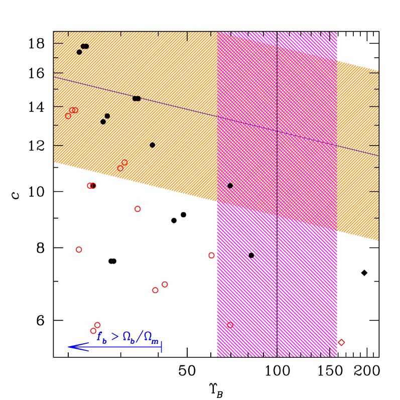
Figure 1: Dark matter (NFW) concentration versus total mass-to-light ratio at the virial radius, $r_{200}$ (open circles) and $r_{102}$ (filled circles), as inferred from the orbit solutions of Romanowsky et al. (2003, supporting online material, circles) and Romanowsky (2005, private communication, diamonds), using equation (66). The oblique horizontal line indicates the concentration-mass that we infer in paper I from the dissipationless $\Lambda$CDM simulations of Navarro et al. (2004), while the vertical line gives the mass-to-light ratio at the virial radius from the cosmoslogical prediction of Marinoni & Hudson (2002). The hashed regions give an indication of the uncertainties on the concentration-mass relation (factor 1.4) and the mass-to-light ratio at the virial radius derived by Marinoni & Hudson (factor 1.6). The arrow indicates where the solutions lead to a baryonic fraction that is higher than the universal value. The filled symbols ought to lie within the hatched regions and to the right of the arrow.

Whereas Romanowsky et al. quote $\Upsilon_{B}=33\pm 14$ at 120 kpc, we find, using the same input values of $r_{s}$, $v_{*}$, $v_{s}^{2}/v_{*}^{2}$, assuming $R_{e}=36^{\prime\prime}$, (from which we infer a Hernquist scale radius of $a=1.0\,\rm kpc$), $\Upsilon_{B}(120\,\hbox{kpc})$ to be in the range $19-48$, with a mean of 27 and a median of 22. Extrapolating to the virial radius, defined in this paper as $r_{200}$, we find $\Upsilon_{B}$ in the range 20 to 70, with a mean of 32 and a median of 25, while for the $\Lambda$CDM virial radius, $r_{102}$, we get $\Upsilon_{B}$ between 22 and 82, with a mean of 37 and a median of 28.

Figure 1 shows that one of the 15 orbit solutions of Romanowsky et al. has a combination of virial mass-to-light ratio and concentration parameter in line with the predictions from dissipationless cosmological simulations ($\Upsilon_{B,102}=70$ and $c=10$), where the concentration parameter predictions are those that Napolitano et al. (2005) rederived from the dissipationless cosmological simulations analyzed by Bullock et al. (2001). None of the orbit solutions lead to the very low concentration parameters favoured by Borriello et al. (2003) and Napolitano et al..

We also note that the Hernquist model contribution to the mass-to-light ratio at the virial radius is always near $\Upsilon_{*,B}=5.6$. According to equation (28), this amounts to a minimum mass-to-light ratio of $\Upsilon_{B}=41$ for the baryonic fraction at the virial radius to be equal to the universal value. Only three of the fifteen orbit solutions of Romanowsky et al. can be modelled with no baryon bias, but for their mean value of $\Upsilon_{B}=33$, which we adopt as our lower limit, the baryon bias is (eq. [29]) $b_{b}=1.25$ with $\Upsilon_{*,B}=5.6$ or $b_{b}=1.45$ with $\Upsilon_{*,B}=6.5$. Therefore, in systems with total mass-to-light ratios as low as the mean derived by Romanowsky et al., the baryon fraction within the virial radius is greater than the universal value, unless the stellar mass-to-light ratio is overestimated (see also Napolitano et al., 2005). One is then left with the difficulty of explaining how baryons can segregate from dark matter as far out as the virial radius.

3.2 Velocity anisotropy

Given the mass / anisotropy degeneracy mentioned in Sect. 1, it is difficult to estimate the radial variation of the anisotropy parameter, $\beta$ (defined in eq. [2]). The simplest solution is to assume isotropy throughout the galaxy. In fact, for clusters of galaxies, Merritt (1987), Łokas & Mamon (2003) and Katgert et al. (2004) each derived isotropic orbits throughout, Merritt and Katgert et al. by examining the global velocity distribution and Łokas & Mamon by performing a joint local analysis of the radial profiles of the line-of-sight velocity dispersion and kurtosis. With their Schwarzschild-like Gerhard et al. (1998) modelling of elliptical galaxies, Kronawitter et al. (2000) and Saglia et al. (2000) find $\beta\mathrel{\hbox{\hbox to0.0pt{\hbox{\lower 4.0pt\hbox{$\sim$}}\hss}\hbox{$<$}}}0.3$ within $R_{e}/2$.

It is useful to compare these still very uncertain anisotropy estimates with those measured in cosmological $N$-body simulations. Figure 2 shows the anisotropy profiles for five recent analyses of dissipationless cosmological simulations by Diaferio (1999), Colín et al. (2000), Rasia et al. (2004), Diemand et al. (2004b), and Wojtak et al. (2005), with the latter four converted from $r/r_{100}$ to $r/r_{200}$ assuming $r_{100}/r_{200}=1.37$, as expected for Nav04 models with the masses (at the level of galaxy clusters) as simulated. Note that the orbital anisotropies of Diaferio (1999), Colín et al. (2000), and Wojtak et al. (2005) include the mean radial and tangential streaming motions, while that of Rasia et al. (2004) does not.

The Figure also displays analytical representations of the data: the model (dotted curve) that Carlberg et al. (1997) fit to the kinematics of CNOC clusters:

$$\beta(r)=2\,\beta_{m}\,{r_{a}\,r\over r^{2}+r_{a}^{2}}\ ,$$ (67)

with $\beta_{m}=0.65$ and $r_{a}=2\,r_{v}$, which Colín et al. (2000) found to fit well the anisotropy of the subhalos in their simulation, as well as an anisotropy model that also appears to fit well the simulation data:

$$\beta(r)={1\over 2}\,{r\over r+r_{a}}\ ,$$ (68)

for $r_{a}=0.18$ (lower solid curve).

The anisotropy profiles plotted in Figure 2 are for all the particles of a halo, instead of for the subhalos of a halo, which are much closer to isotropy. Indeed, we are wary of using the subhalos in the cosmological simulations, because the number density profile of subhalos within halos is suspicious, as it has a much shallower inner slope than the dark matter (Colín et al., 1999) with a nearly homogeneous core (Diemand et al., 2004a), in contrast with the distribution of galaxies in clusters (Carlberg et al., 1997). Interestingly, stars show more radial orbits than dark matter particles in hydrodynamical cosmological (Sáiz et al., 2004) and merger (Dekel et al., 2005) simulations, where the gas is allowed to cool and form stars, and, for the latter study, have a feedback effect on the cooling of the remaining gas. Dekel et al. find a stellar anisotropy profile that resembles the model of equation (68), with $r_{a}\simeq 1.4\,R_{e}\simeq 0.018\,r_{v}$ (using eq. [44] for the latter approximation). This is shown as the higher of the two solid curves in Figure 2.

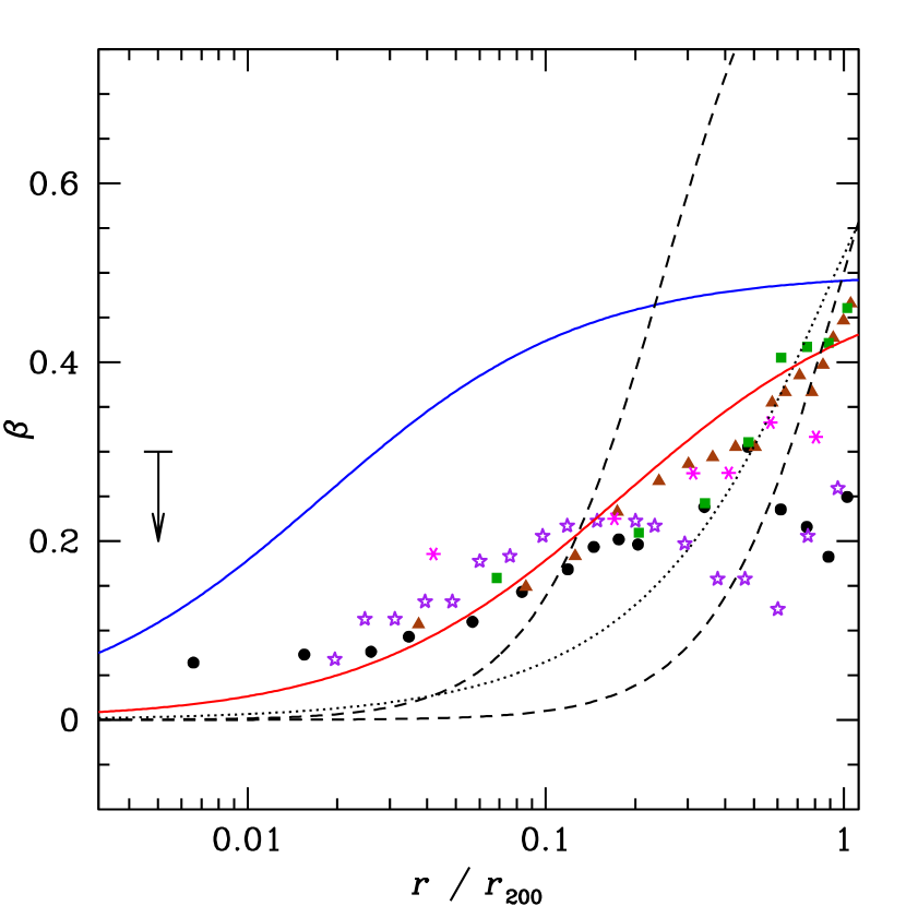
Figure 2: Radial variation of the velocity anisotropy found in cosmological $N$-body simulations. The asterisks, triangles, stars, circles, and squares correspond to particles within halos of cosmological $\Lambda$CDM $N$-body simulations of Diaferio (1999), Colín et al. (2000), Rasia et al. (2004), Diemand et al. (2004b), and Wojtak et al. (2005), respectively. The dotted curve is the profile proposed by Carlberg et al. (1997) (eq. [67]) and found by Colín et al. to fit well the subhalo anisotropies. The solid curves are the analytical fit of equation (68), with $r_{a}/r_{v}=0.18$ (providing a good fit to the data from the dissipationless cosmological $N$-body simulations) and 0.018 (matching the anisotropy profile of Dekel et al.’s 2005 merger remnants), going upwards (red and blue in the electronic version of the journal). The dashed curves are the Osipkov-Merritt anisotropy (eq. [69]) with $r_{a}/r_{v}=0.25$ and 1, going downwards. The upper limit is from the analysis of Kronawitter et al. (2000) and Saglia et al. (2000), assuming $r_{v}/R_{e}\simeq 100$ as expected for our standard parameters ($L_{B}=10^{10}\,h_{70}{\rm L_{\odot}}$ and $\Upsilon_{B}=100$).

Figure 2 indicates that the anisotropy of equation (68) with $r_{a}=0.18\,r_{v}$ fits very well the anisotropy profiles of Colín et al., Rasia et al., and Diemand et al. (2004b) from 2% to 10% of the virial radius, which happens to be the region where we shall find that the anisotropy may play an important role in modelling the mass-to-light ratios of elliptical galaxies. Figure 2 also shows the commonly-used Osipkov-Merritt (Osipkov, 1979; Merritt, 1985) anisotropy model,

$$\beta(r)={r^{2}\over r^{2}+r_{a}^{2}}\ ,$$ (69)

for $r_{a}/r_{v}=0.25$ and 1. Clearly, the Osipkov-Merritt anisotropy is a poor fit to the simulations, as it converges to a too high value of unity, and worse, decreases to zero too fast at increasingly low radii.

In what follows, we generally assume that the anisotropy of the stellar population is equal to the anisotropy of the dark matter particle system, but we will also allow for the much stronger radial anisotropy found by Dekel et al.. In appendix A, we derive the line-of-sight velocity dispersion profile for four different anisotropy profiles: constant anisotropy, the limiting purely radial case, Osipkov-Merritt, and the anisotropy model of equation (68). With these single quadratures, one avoids double integration (first integrating the Jeans equation to obtain the radial velocity dispersion, and then integrating along the line of sight to get the line-of-sight velocity dispersion).

4 Results

If, as we found in paper I, the mass models found in dissipationless cosmological $N$-body simulations are not able to reproduce by themselves the rather high central velocity dispersions observed in elliptical galaxies, this suggests that the central velocity dispersions of ellipticals are dominated by the stellar component and by a central supermassive black hole, as we shall see below. We are now left with the question of whether the NFW, JS–1.5 and Nav04 models are adequate in describing the diffuse dark matter component (excluding the central black hole) of elliptical galaxies.

Dark matter is expected to become significant in the outer regions of ellipticals, since the black hole affects the central regions, and the influence of the stellar component is usually thought to be important in the inner regions, at least within $R_{e}$. We therefore predict the line-of-sight velocity dispersion profiles of ellipticals built with 4 components: a Sérsic stellar component of constant mass-to-light ratio $\Upsilon_{*}$, a central black hole, a hot gas component, and a diffuse dark matter component described by an NFW, JS–1.5, or Nav04 model, according to our parameterisations of Sec. 2. We focus our analysis on the following set of parameters: a luminosity $L_{B}=L_{*,B}=1.88\times 10^{10}\,h_{70}^{-2}\,{\rm L_{\odot}}$ (implying $R_{e}=3.2\,h_{70}^{-1}\,\rm kpc$ from eq. [15], $m=3.15$ from eq. [16], and $a_{S}=12\,h_{70}^{-1}\,\rm pc$ from eq. [17]), a stellar mass-to-light ratio $\Upsilon_{*,B}=6.5$ and no baryon bias ($b_{b}=1$).

4.1 The effects of velocity anisotropy

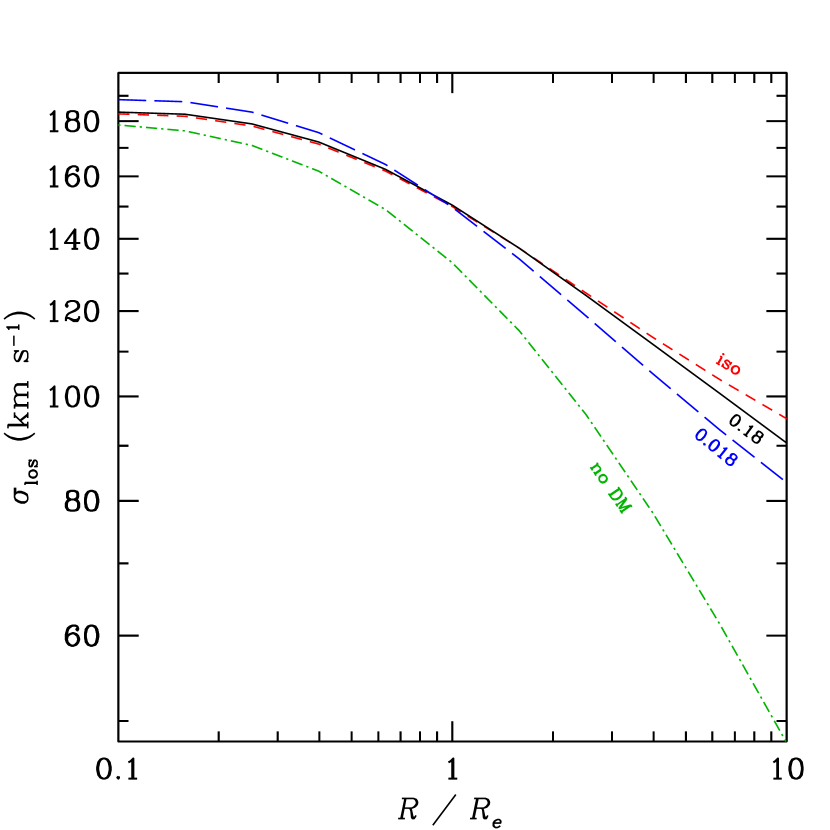
Figure 3: Line-of-sight stellar velocity dispersion of 4-component elliptical galaxy for different anisotropy models (eqs. [88] and [85]), with a Nav04 dark matter model, $L_{B}=L_{*,B}=1.88\times 10^{10}{\rm L_{\odot}}$, $m=3.15$, $R_{e}=3.2\,h_{70}^{-1}\,\rm kpc$, $\Upsilon_{*,B}=6.5$, $\Upsilon_{B}=100$, $g_{\rm BH}=0.0015$ and $b_{b}=1$. The short-dashed, solid, and long-dashed curves represent the isotropic (see eq. [80]), mildly and sharply anisotropic (eq. [68], with $r_{a}/r_{v}=0.18$ and 0.018), using equation [78]), respectively, while the dash-dotted curve represents a galaxy with no dark matter ($\Upsilon_{B}=f_{b}\,\Upsilon_{B}^{\rm std}=14$) and mild anisotropy (eq. [68] with $r_{a}/r_{v}=0.18$) — these four cases are respectively shown in red, black, blue and green in the electronic version of the journal.

We first check the effects of anisotropy, by computing the line-of-sight velocity dispersions of our four-component model, assuming different anisotropy profiles. Figure 3 shows the total line-of-sight velocity dispersion (i.e., the quadratic sum of the individual velocity dispersions of the four components) for four anisotropy models: isotropic, radial, and the model of equation (68) for two choices of $r_{a}$. The line-of-sight velocity dispersion profile of the anisotropy model of equation (68) with our standard value of $r_{a}=0.18\,r_{v}$ is virtually indistinguishable from that of the isotropic model: the anisotropic model producing 2% lower velocity dispersions at $5\,R_{e}$. On the other hand, if the velocity ellipsoid is indeed radially anisotropic beyond $r_{v}/50$, as suggested by the orbital anisotropies of the stellar particles in the simulations of Sáiz et al. (2004) and Dekel et al. (2005), then one can obtain a small but non-negligible decrement in line-of-sight velocity dispersion: if $r_{a}=0.018\,r_{v}$, one finds decrements of 4% at $2\,R_{e}$ and 9% at $5\,R_{e}$. Note that with Osipkov-Merritt anisotropy, and $r_{a}=r_{v}$ or even $r_{a}=0.25\,r_{v}$, the line-of-sight velocity dispersions (obtained with eq. [81]) are indistinguishable from the isotropic ones.

Hence, with an optimistic precision on velocity dispersion of $5\,\,\rm km\,s^{-1}$, the slight radial anisotropy found in cosmological $N$-body simulations produces line-of-sight velocity dispersion profiles that are virtually indistinguishable within $9\,R_{e}$ from analogous profiles assuming velocity isotropy everywhere, while the stronger radial anisotropy found for stars in simulated merger remnants displays measurable differences beyond $2\,R_{e}$.

In comparison, as illustrated in Figure 3, discarding the dark matter component has a much stronger effect on the velocity dispersions at a few effective radii than does the strong radial anisotropy with $r_{a}=0.018\,r_{v}$, with dispersion 19% and 33% lower than with dark matter (at $\Upsilon_{B}=100$).

4.2 Relative importance of dark matter, stars, gas and the central black hole

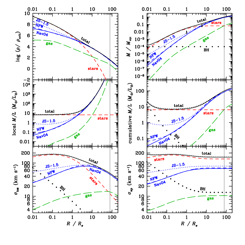
Figure 4: Contribution of stars (short dashes), dark matter (light curves; dashed for NFW, dotted for JS–1.5, and solid for Nav04), hot gas (long dashes), and the central black hole (big dots) to the local mass density (upper left), cumulative mass (upper right), local (middle left) and cumulative (middle right) mass-to-light ratios, mildly anisotropic (eq. [68] with $r_{a}=0.18\,r_{v}$) line-of-sight velocity dispersion (lower left) and isotropic aperture velocity dispersion (lower right); for a giant elliptical with $L_{B}=L_{*,B}=1.88\times 10^{10}h_{70}^{-2}{\rm L_{\odot}}$ (corresponding to $m=3.12$, $R_{e}=3.2\,h_{70}^{-1}\,\rm kpc$ and $a_{S}=11.6\,h_{70}^{-1}\,\rm pc$), $\Upsilon_{*,B}=6.5$, $\Upsilon_{B}=100$ (i.e., $b_{\Upsilon,B}=0.26$), yielding $r_{v}/R_{e}=79$, shown as the thin vertical lines) with no baryon bias ($b_{b}=1$), black hole to stellar mass ratio $g_{\rm BH}=0.0015$ and dark matter scaling relations from Sec. 2. The top, solid and dotted, curves represent the total galaxy assuming either Nav04 or JS–1.5 dark matter, respectively. The arrows (upper right) indicate the lower limits to the dark matter mass according to Loewenstein & White (1999), given our total mass at those radii.

Figure 4 shows the contribution of each component to the local mass density, cumulative mass, line-of-sight (with the mild anisotropy of eq. [68] and $r_{a}/r_{v}=0.18$) and aperture (isotropic) velocity dispersions. For our standard parameters, $L_{B}=L_{*,B}=1.88\times 10^{10}\,h_{70}^{-2}{\rm L_{\odot}}$, $\Upsilon_{*,B}=6.5$, $\Upsilon_{B}=100$ (the typical value inferred in the cosmological analyses of Marinoni & Hudson, 2002 and Yang et al., 2003, i.e. $b_{\Upsilon}=0.26$), and $g_{\rm BH}=0.0015$, the stellar component dominates over the dark matter component out to $R\simeq 2\,R_{e}$ for the local density, $5\,R_{e}$ for the enclosed mass, $3\,R_{e}$ for the line-of-sight velocity dispersion, while the stars dominate the dark matter everywhere for the aperture velocity dispersion. In the inner regions, with $g_{\rm BH}=0.0015$, the central black hole is the dominant component for $R<0.015\,R_{e}$ for the enclosed mass, $0.006\,R_{e}$ for the aperture velocity dispersion, but only out to $0.003\,R_{e}$ (i.e., $\simeq 10\,\rm pc$) for the line-of-sight velocity dispersion.

The figure also indicates that our model produces Nav04 dark matter contents that at $R=5\,R_{e}$ are consistent with the joint kinematics / X-ray modelling of Loewenstein & White (1999), while our Nav04 dark matter mass fraction at $R=R_{e}$ is 1.6 times lower than the lower limit found by Loewenstein & White (but our predicted JS–1.5 dark matter mass is precisely the lower limit of Loewenstein & White).

Although the gas component begins to dominate the stellar component at $10\,R_{e}$, as expected, the gas does not influence the line-of-sight or aperture velocity dispersions: although its influence on the line-of-sight velocity dispersion dominates that of the stellar component at $60\,R_{e}$, by that large radius the dark matter component is fully dominating the stellar velocity dispersion.

Given the strong dominance of stars (and the central black hole) over the dark matter component, the differences in aperture or line-of-sight velocity dispersion profiles between the inner dark matter slopes of $\alpha=1$ and $\alpha=3/2$ are very small, and basically indistinguishable from observations.

The line-of-sight velocity dispersion using the Nav04 profile is also indistinguishable from the other two dark matter profiles. However, the Nav04 profile produces slightly ($5\%$) lower total velocity dispersions at $R=5\,R_{e}$. This is illustrated in Figure 5, which plots the mass and line-of-sight velocity dispersion profiles normalized to those of the Nav04 model. At radii around $r_{v}/8$ (corresponding to $10\,R_{e}$ for our standard set of parameters), the NFW velocity dispersion is up to 6% larger than that of the Nav04 model, which fits much better the density profiles found in dissipationless cosmological $N$-body simulations. The corresponding overestimate of the cumulative mass is almost 20% at $r_{v}/8$ ($10\,R_{e}$), and the same effect is visible in Figure 2 of Navarro et al. (2004) (with the virial radii given in their Table 3).

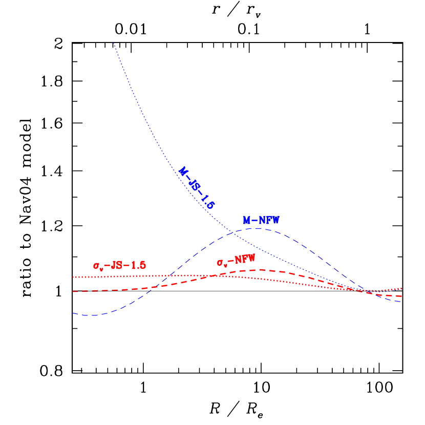
Figure 5: Radial profiles of cumulative dark mass (thin curves, blue in the electronic version of the Journal) and stellar line-of-sight velocity dispersion (thick curves, red in the electronic version of the Journal) for the NFW (dashed curves) and JS–1.5 (dotted curves) dark matter models, both normalized to those of the Nav04 dark matter model. Same parameters as in Figure 4.

The maximum velocity dispersion ratio in Figure 5 indicates that the lower stellar velocity dispersions obtained with the Nav04 dark matter model relative to its NFW counterpart are not caused by the convergent dark matter mass profile of the former at large radii, but by the 20% difference in mass profiles at $10\,R_{e}$.

The conclusions from Figure 4 are unchanged if we adopt the much higher universal total mass-to-light ratio $\Upsilon_{B}=\overline{\Upsilon}_{B}=390$, instead of 100, in particular the stellar component dominates the dark matter out to only $2\,R_{e}$ (instead of $3\,R_{e}$) for the line-of-sight velocity dispersion.

Note that the ratio of aperture velocity dispersion at $R_{e}/8$ (the aperture used by Jorgensen et al., 1996) to circular velocity at the virial radius, $\sigma_{\rm ap}(R_{e}/10)/V_{v}$, is 0.64 when $\Upsilon_{B}=390$, but as high as 1.00 when $\Upsilon_{B}=100$. Indeed, since the stars dominate the aperture velocity dispersion measurement, decreasing the total mass-to-light ratio decreases $V_{v}$ without affecting much $\sigma_{\rm ap}(R_{e}/8)$.

Figure 6 displays radial profiles of the baryon fraction and gas-to-star ratio.

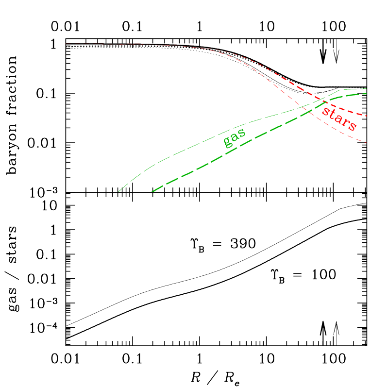
Figure 6: Radial profiles of cumulative fractions of gas (long dashes), stars (short dashes) and total baryons (solid curve) for a Nav04 dark matter model (top), and the cumulative gas/star ratio (bottom). Also shown is the baryon fraction with the JS–1.5 model (dotted in top panel). The arrows indicate the virial radii. Thick and thin curves and arrows are for $\Upsilon_{B}=100$ and 390, respectively. Other parameters are the same as in Figure 4.

For our standard mass-to-light ratio at the virial radius, $\Upsilon_{B}=100$, the decrease in star fraction with radius is only partially compensated by the increase in gas fraction, so that the total baryon fraction decreases with radius for $r<r_{v}$: for the Nav04 model, $f_{b}$ decreases from unity at small radii to 0.87 at $R_{e}$, 0.76 at $2\,R_{e}$, 0.53 at $5\,R_{e}$, and down to a minimum of 0.132 at $R=68\,R_{e}\simeq 0.95\,r_{v}$, and then slowly rises by 0.1% from there to the virial radius. These trends are very similar for the NFW dark matter model, while for the JS–1.5 dark matter model, the baryon fraction actually increases from 0.87 at $R_{e}/100$ to 0.90 at $R_{e}/13$, then decreases to 0.80 at $R_{e}$, 0.70 at $2\,R_{e}$, 0.49 at $5\,R_{e}$. For the universal mass-to-light ratio, $\Upsilon_{B}=390$, the trends are similar, except that the baryonic fraction reaches a minimum of 0.10 (for all dark matter models) around $50\,R_{e}$, i.e, $r_{v}/2$, and rises at larger radii.

The bottom plot of Figure 6 indicates that the gas-to-star ratio rises, roughly as $r^{1.2}$ from $r_{v}/10\,000$ to $r_{v}$. If the mass-to-light ratio at the virial radius is increased, while the baryonic fraction at the virial radius and the total stellar mass are kept constant, then the gas component must become relatively more important, which explains why the $\Upsilon_{B}=390$ gas-to-star ratio is larger than the $\Upsilon_{B}=100$ gas-to-star ratio, by a factor $390/100=3.9$.

4.3 Can one weigh the dark matter component?

As we have seen in paper I and Sect. 4.2, the dark matter contributes little to the inner regions of elliptical galaxies, and hence we need to focus on the outer regions to be able to weigh the dark component.

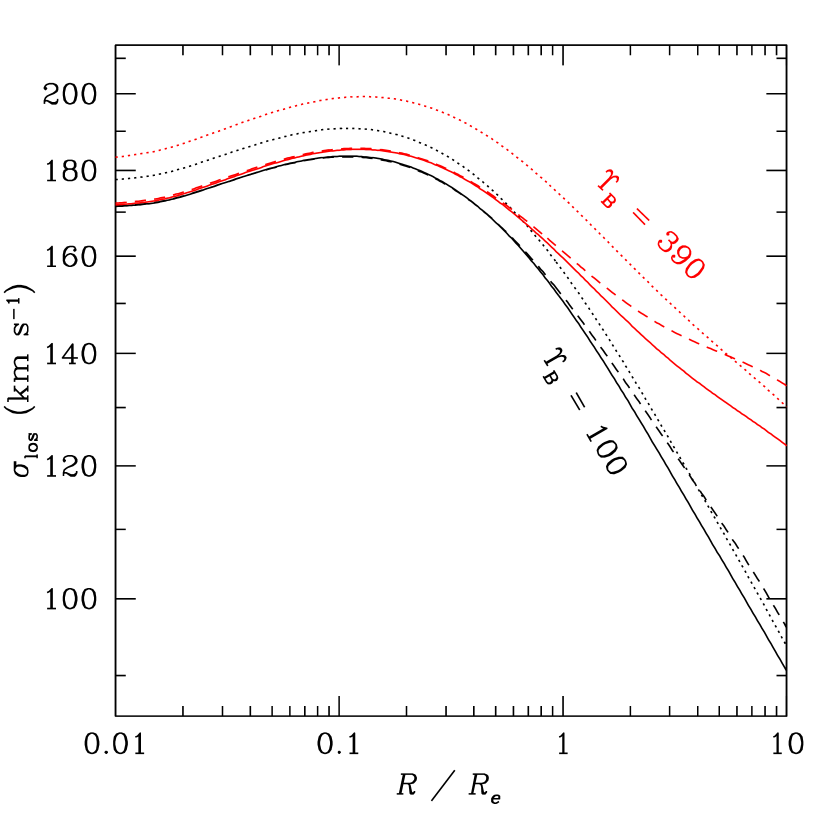
Figure 7: Line-of-sight stellar velocity dispersions of our 4-component elliptical galaxy (eq. [78]) for our slightly anisotropic (eq. [68] with $r_{a}=0.18\,r_{v}$) NFW (dashed), JS–1.5 (dotted) and Nav04 (solid) dark matter models, with total mass-to-light ratio within the virial radius $\Upsilon_{B}=100$ and 390, increasing upwards (respectively black and red in the electronic version of the Journal). Same other parameters as Figure 4.

Figure 7 illustrates the effect of the mass of the dark matter component on the line-of-sight velocity dispersion profiles. While the steep inner slope of the density profile of the JS–1.5 model allows it to have a non-negligible effect on the line-of-sight velocity dispersions at small projected radii, the opposite is true for the NFW and Nav04 models: the inner line-of-sight velocity dispersions are completely independent of the total mass of the galaxy. Moreover, at large radii with $\Upsilon_{B}=100$, it is difficult to distinguish between the three dark matter models. Note that relative to the Nav04 dark matter model, the NFW model has no effect on the line-of-sight velocity dispersions measured from 0.01 to $0.1\,R_{e}$ (even when no central black hole is present), while the JS–1.5 component has a small effect, increasing with mass.

Figure 8 shows again the effect of the mass of the dark matter component, this time allowing the very low mass-to-light ratio deduced by Romanowsky et al. (2003) (see Sect. 3.1), which requires $b_{b}>1$ (eq. [29]).

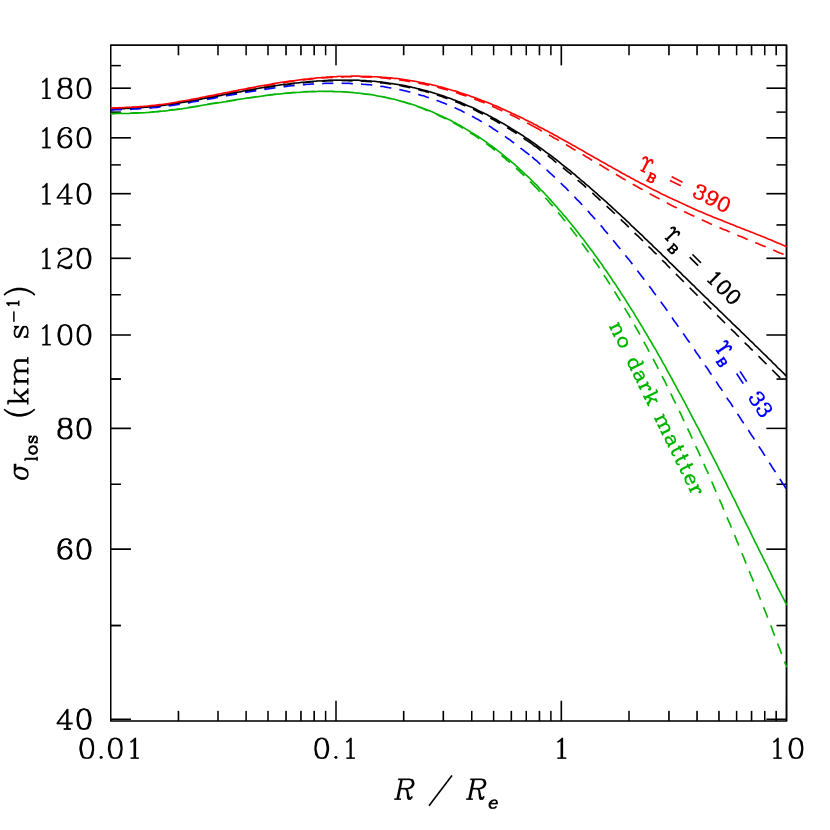
Figure 8: Same as Figure 7 with Nav04 dark matter, $\Upsilon_{B}=33$, 100, and 390, increasing upwards (blue, black, and red in the electronic version of the Journal), as well as no dark matter ($\Upsilon_{B}=f_{b}\,\Upsilon_{B}^{\rm std}=14$) case (lower curve, green in the electronic version of the Journal), for which $\Upsilon_{B}=f_{b}\,\Upsilon_{B}^{\rm std}=14$. The baryon bias is $b_{b}=1$ (solid curves) and $b_{b}=1.5$ (dashed curves). The case $b_{b}=1$ is not shown for $\Upsilon_{B}=33$ because the gas fraction would then be negative (see eq. [28]). Same other parameters as in Figure 4.

The figure shows that, at $R/R_{e}=2$, 3, 4, 5, and 6, the velocity dispersion increases by 26, 33, 39, 43, and $46\,\rm km\,s^{-1}$ when the mass-to-light ratio at the virial radius is increased from $\Upsilon_{B}=33$ to $\Upsilon_{B}=390$. In other words, a line-of-sight velocity dispersion measurement at $4\,R_{e}$ with $20\,\rm km\,s^{-1}$ measurement error implies an uncertainty on the total mass-to-light ratio of a factor greater than 3! At higher radii, less precision is required on the velocity dispersions, but these are more difficult to estimate as they are smaller. These conclusions are the same if we adopt purely isotropic models. This three-fold uncertainty becomes even larger if we do not assume a precise form for the velocity anisotropy profile.

Also shown in Figure 8 is the case of no dark matter (for which $\Upsilon_{B}=f_{b}\,\Upsilon_{B}^{\rm std}=14$). The dispersions now fall to quite low values. However, this ‘no dark matter’ case is extreme, as its baryonic fraction is unity.

How much do these conclusions depend on the galaxy luminosity? Figure 9 displays the dispersion profiles normalized to the values at $0.1\,R_{e}$ (at which radius the dispersion profile is fully dominated by the stellar component, as seen in Fig. 4).

Figure 9: Normalized line-of-sight stellar velocity dispersion for our slightly anisotropic (eq. [68] with $r_{a}=0.18\,r_{v}$) model with Nav04 dark matter, with $\Upsilon_{B}=100$ and $L_{B}=3.2\times 10^{9}$ (dotted curve), $10^{10}$ (solid curve), and $3.2\times 10^{10}{\rm L_{\odot}}$ (dashed curve), with Sérsic shape $m$ and effective radius $R_{e}$ taken from equations (16) and (15), respectively, and other parameters as in Figure 4.

The velocity dispersion profiles have a strikingly similar shape, with relative differences less than 6.5% for $R<5\,R_{e}$, and interestingly, less than 3.5% for $R\simeq 2.5\,R_{e}$. Also, the slope at $R>R_{e}$ varies with luminosity.

Reverting now to our standard luminosity $L_{B}=L_{*,B}=1.88\times 10^{10}{\rm L_{\odot}}$, we look in more detail at how the velocity dispersion at a fixed number of effective radii scales with the total mass-to-light ratio. Figure 10 shows that the velocity dispersion at 2 and $5\,R_{e}$ rises slowly with mass-to-light ratio, as a power-law of slope $1/13$ and $1/6$, respectively.

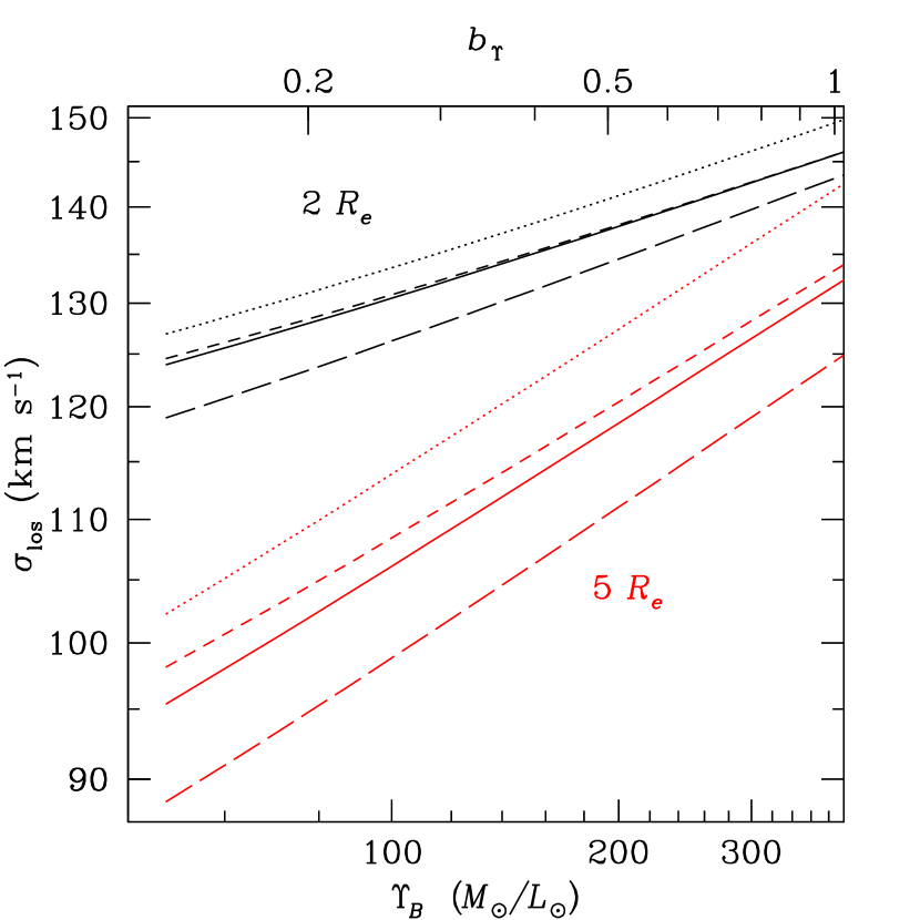
Figure 10: Line-of-sight stellar velocity dispersion of our 4-component elliptical galaxy at 2 (upper curves) and 5 (lower curves) effective radii, as a function of total mass-to-light ratio at the virial radius (or its bias relative to the universal value, upper axis). The dotted, short-dashed, solid and long-dashed curves represent the isotropic NFW, isotropic Nav04 and anisotropic (eq. [68]) Nav04 models, respectively, the latter two with $r_{a}/r_{v}=0.18$ and 0.018, respectively. Same parameters as in Figure 4, in particular no baryon bias ($b_{b}=1$), which limits the virial mass-to-light ratios as in equation (28).

In other words, the virial mass-to-light ratio increases very sharply with the measured line-of-sight velocity dispersion at a fixed number of effective radii. Also, at fixed measured velocity dispersion, the standard isotropic NFW model produces significantly smaller mass-to-light ratios than the anisotropic Nav04 model.

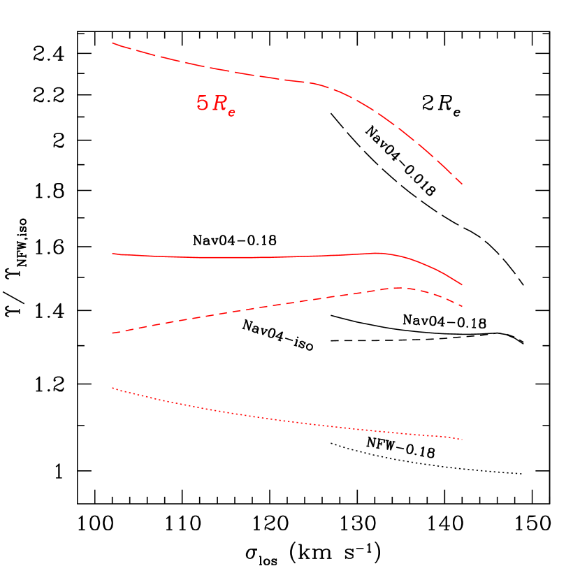
Figure 11: Ratio of the mass-to-light ratio inferred from a general model to the mass-to-light ratio inferred from the isotropic NFW model, as a function of the measured line-of-sight velocity dispersion at 5 (left) and 2 (right) effective radii for a continuous range of virial mass-to-light ratios. The short-dashed, solid and long-dashed curves represent the ratios to isotropic NFW mass-to-light ratios for the isotropic Nav04 and anisotropic (eq. [68]) Nav04 models, respectively, the latter two with $r_{a}/r_{v}=0.18$ and 0.018, respectively, while the dotted curve shows the analogous ratio for the anisotropic NFW model (eq. [68] with $r_{a}=0.18\,r_{v}$). Same parameters as in Figure 4.

This is quantified in Figure 11: At $5\,R_{e}$, going from the isotropic NFW model to the isotropic Nav04 model, the inferred mass-to-light ratio is $\simeq 1.4$ times higher (left ‘Nav04-iso’ curve), and this factor is roughly independent of the measured velocity dispersion. Indeed, as seen in Figure 5, at $5-20\,R_{e}$, the velocity dispersion of the NFW model is a few percent larger than that of the Nav04 model. One therefore needs a higher mass-to-light ratio to reproduce a fixed value of $\sigma_{\rm los}$ with the Nav04 model in comparison with the less accurate NFW model. Moreover, going from the isotropic NFW (Nav04) model to the slightly anisotropic NFW (Nav04) model of equation (68), the inferred mass-to-light ratio is 1.1 to 1.2 times larger (increasing for smaller measured velocity dispersions), again as expected since radial anisotropy causes lower values of $\sigma_{\rm los}$ at large radii (see Fig. 3). The combined effect of dark matter model and velocity anisotropy is displayed in the upper curve of Figure 11, and indicates that line-of-sight velocity dispersion measurements lower than $135\,\rm km\,s^{-1}$ for an $L_{*}$ elliptical galaxy imply an underestimation of the mass-to-light ratio within the virial radius of a factor of roughly 1.6, when using the isotropic NFW model instead of the best slightly anisotropic models arising from dissipationless cosmological $N$-body simulations. Similarly, the velocity dispersion at $5\,R_{e}$ produced by the Nav04 dark matter model with the strong radial stellar anisotropy ($r_{a}=0.018\,r_{v}$) seen by Dekel et al. in merger simulations is the same as that produced by an isotropic NFW dark matter model with a virial mass-to-light ratio 2.3 times lower.

Similar patterns are found at $2\,R_{e}$ but with considerably smaller effects. Note that a positive baryon bias ($b_{b}>1$) will produce lower velocity dispersions at a given radius for a given mass-to-light ratio (Fig. 8), hence the inferred mass-to-light ratio will be increased relative to the value obtained for $b_{b}=1$.

How far out should one measure velocity dispersions? Table 1 compares the uncertainties at 2 and $5\,R_{e}$, from the two effects we discussed above: 1) the observational uncertainty on the velocity dispersion as inferred from the slopes of the curves in Figure 10, and 2) the uncertainty caused by uncertain total (or equivalently dark) mass and anisotropy profiles, as inferred from Figure 11, where we assume the velocity dispersion profile given in Figure 10 and guess the measurement errors (see also Sect. 5, below).

Table 1: Relative uncertainties on the mass-to-light ratio at the virial radius

$R$	$\sigma_{v}$	$\delta\sigma_{v}$	$\displaystyle\left({\delta\Upsilon\over\Upsilon}\right)_{\rm obs}$	$\displaystyle\left({\delta\Upsilon\over\Upsilon}\right)_{\rm mod}$	$\displaystyle\left({\delta\Upsilon\over\Upsilon}\right)_{\rm tot}$
	$(\,\rm km\,s^{-1}$)	$(\,\rm km\,s^{-1})$
$2\,R_{e}$	130	5	0.9	1.0	1.3
$5\,R_{e}$	106	20	1.8	1.4	2.3
$5\,R_{e}$	106	10	0.7	1.4	1.6

For assumed measurement errors on $\sigma_{\rm los}$ of $5\,\rm km\,s^{-1}$ at $2\,R_{e}$ and $20\,\rm km\,s^{-1}$ at $5\,R_{e}$, we end up with a total factor of 2.3 at $2\,R_{e}$ and of 3.3 at $5\,R_{e}$, the latter factor being reduced to 2.6 if the velocity dispersion at $5\,R_{e}$ can be measured with $10\,\rm km\,s^{-1}$ accuracy.

Of course, one can do better by combining the measurements of $\sigma_{\rm los}$ at various radii between 1 and $5\,R_{e}$. A quantitative assessment of combining measurements is beyond the scope of the present paper. However, inspection of the lower left panel of Figure 4, indicates that the logarithmic slope of the line-of-sight velocity dispersion profile is roughly independent of the limiting radii, when these lie in the interval $[1,20]\,R_{e}$. The middle right panel of Figure 4 shows that this is not the case for the (cumulative) mass-to-light ratio: the slope rises with radius. In view of the possible $1.3$ (or more) underestimation of the effective radius of NGC 3379, any error on estimating the effective radius of a galaxy will lead to biases in analyses based upon the mass-to-light ratio gradient, such as the study of Napolitano et al. (2005).

It is much safer to base one’s analysis on the velocity dispersion gradient. Figure 12 shows that the logarithmic slope of the line-of-sight velocity dispersion profile decreases linearly with the log of the mass-to-light ratio at the virial radius.

Figure 12: Logarithmic slope of the radial profile of the line-of-sight stellar velocity dispersion a a function of the total mass-to-light ratio at the virial radius. Same line types as in Fig. 10.

Alas, the direct interpretation of this logarithmic slope is complicated by the uncertainties in the dark mass and stellar anisotropy profiles: for a given slope of the velocity dispersion profile, these uncertainties lead to a factor 3 uncertainty on the mass (or mass-to-light ratio) at the virial radius. Moreover, as noted earlier (Fig. 9) the luminosity of the galaxy also affects the slope of the line-of-sight velocity dispersion profile.

The large range of mass-to-light ratios at the virial radius that we infer from Romanowsky et al.’s 15 orbit solutions (Fig. 1) suggests that the detailed orbit modelling provides little constraint on the dark matter content of ellipticals within their virial radii.

5 Summary and discussion

In this paper, a 4-component model of elliptical galaxies has been built to compare the predictions of cosmological $N$-body simulations with the observations of elliptical galaxies. The inner regions are dominated by the stellar component, unless the inner dark matter density profile is as steep as $r^{-3/2}$, which seems to disagree with the latest cosmological $N$-body simulations of Stoehr et al. (2002), Power et al. (2003), Navarro et al. (2004), Diemand et al. (2004a), and Stoehr (2006). Therefore, there is little hope in constraining, through the analysis of internal kinematics, the inner slope of the dark matter density profile unless it is as large as $3/2$ in absolute value.

The dark matter component is found to become important at typically 3–5 effective radii. At these radii, the galaxy surface brightness is low and one requires the sensitivity of an 8m-class telescope, and the required precision on velocity dispersion of say $5\,\rm km\,s^{-1}$ imposes a decent spectral resolution (with $R=1000$, a signal-to-noise ratio $S/N>10$ should lead to $10\,\rm km\,s^{-1}$ precision on observed velocity dispersions — L. Campbell, private communication). For example, according to the Exposure Time Calculator at the ESO Web site, observations of the giant elliptical galaxy NGC 3379, using the the Sérsic surface brightness profile we fit (see Sect. 3.1), on the VLT-UT1 (Antu) 8m telescope using the FORS2 multi-slit spectrograph at $R=2000$, one can reach $S/N=10$ (per spectral pixel and per arcsec) in 3 hours at $R=2\,R_{e}$. Among the 16 slits, one can dedicate say 10 for $R=3\,R_{e}$ and the combined spectrum should produce $S/N>10$ with a precision on velocity dispersion of order $5\,\rm km\,s^{-1}$. This measurement at $3\,R_{e}$ should constrain the total mass-to-light ratio within the virial radius, but to fairly low precision: at $3\,R_{e}$, one has ${\rm d}\ln\Upsilon_{B}/{\rm d}\ln\sigma_{v}\simeq 9$, yielding an accuracy of a factor of 1.5 only.

Three physical mechanisms are found to decrease the observed line-of-sight velocity dispersion at 2–5 effective radii:

1. the lower cumulative mass of the new dark matter models such as that of Navarro et al. (2004) at these radii and slightly above;

2. radial velocity anisotropy;

3. a possible excess of the baryon fraction relative to the universal value.

In turn, if we model the observed velocity dispersions at 5 effective radii, the combined effect of the new dark matter models and velocity anisotropy is to increase the inferred mass-to-light ratio at the virial radius by 60% for slight anisotropy, as observed for the particles in structures within dissipationless cosmological $N$-body simulations, and by a factor 2.4 for the strong anisotropy found by Dekel et al. (2005) in simulations of merging galaxies.

The effect of the velocity anisotropy on the mass at the virial radius is a direct illustration of the mass / anisotropy degeneracy. On the other hand, the analysis of the galaxy kinematics at some radius $R$ requires the knowledge of the mass profile beyond $R$ in theory, but just a little beyond $R$ in practice, since the mass profile entering the expression (eq. [84]) for the line of sight velocity dispersion is weighted by the luminosity density profile, which falls relatively fast. Therefore, the extrapolation of the mass profile out to the virial radius depends on the details of the mass profile.

In their analysis of halos from dissipationless cosmological $N$-body simulations, Sanchis, Łokas, & Mamon (2004) showed that the mass profile was recovered to high accuracy beyond $0.03\,r_{v}$. The difference here, is that the line of sight velocity dispersion data in ellipticals extends only out to 2 to 5 effective radii, i.e. to less than 6% of the virial radius, while in clusters of galaxies, the analogous dispersions extend all the way out to the virial radius.

One may be tempted to explain the very low ($\Upsilon_{B}=33$) mass-to-light ratio at the virial radius reported by Romanowsky et al. (2003) (which, at face value requires the baryonic fraction within the virial radius to be larger than the universal value) by this factor of 2.4, which would raise the mass-to-light ratio at $r_{v}$ to $\Upsilon_{B}\approx 80$, and to roughly 100 when we use $r_{102}$ for the virial radius instead of $r_{200}$. However, this comparison is not fair, because the best fitting orbital solutions of Romanowsky et al. are also anisotropic: their orbits are nearly as radial as the stellar orbits at a few $R_{e}$ found by Dekel et al. (A. Romanowsky, private communication).

Furthermore, the low dispersions of planetary nebulae velocities around nearby ellipticals measured by Romanowsky et al., $\approx 80\,\rm km\,s^{-1}$, cannot be reproduced with our models: as seen in Fig. 10, we consistently produce velocity dispersions at $5\,R_{e}$ above $\sigma_{\rm los}=95\,\rm km\,s^{-1}$ for $\Upsilon_{B}>80$. Therefore, resorting to radial anisotropy and to the Nav04 dark matter model appear to be insufficient to explain the low velocity dispersions observed at large radii by Romanowsky et al.. And yet, we found that some of the orbit solutions found by these authors lead to high enough mass-to-light ratios (Fig. 1), as does a new solution (Romanowsky, private communication, and right-most pair of points in Fig. 1). In fact, the 2nd most massive among the solutions of Romanowsky et al. (third pair of points from the right in Fig. 1) has $\Upsilon_{B}(r_{102})=70$, and if a Nav04 dark matter model were used instead of the NFW model, one would get roughly 40% larger masses at the virial radius (see Fig. 11), i.e. 100, as roughly expected from cosmological modelling (Marinoni & Hudson, 2002; Yang et al., 2003). Note that the more massive solutions of Romanowsky et al. have low dark matter concentration parameters, compared with the expectations of Bullock et al. (2001), revised by Napolitano et al. (2005), but one solution ($\Upsilon_{B,102}=70$, $c=10$) is consistent with the predictions from dissipationless cosmological simulations.

Dekel et al. suggest other ways to bring down the velocity dispersions: a steeper density profile for the planetary nebulae measured by Romanowsky et al., and viewing triaxial galaxies along their minor axis. Another possibility is an incomplete dynamical equilibrium of elliptical galaxies, caused by small residual time-variations, affecting both the orbit modelling performed by Romanowsky et al. and the Jeans kinematical modelling, as presented here. Detailed analyses of kinematical observations and of merger simulations are in progress to help clarify the dark matter content of elliptical galaxies.

Appendix A Line-of-sight velocity dispersions for anisotropic models

A.1 Radial velocity dispersion

The general solution to the Jeans equation (1) is

$$\ell(r)\,\sigma_{r}^{2}(r)={1\over f(r)}\,\int_{r}^{\infty}f(s)\,\ell(s)\,{GM(s)\over s^{2}}\,{\rm d}s\ ,$$ (70)

where $f$ is the solution to

$${{\rm d}\ln f\over{\rm d}\ln r}=2\,\beta(r)\ ,$$ (71)

i.e.,

$$f(r)=f(r_{1})\,\exp\left[\int_{r_{1}}^{r}2\,\beta(s)\,{{\rm d}s\over s}\right]$$

(see also van der Marel, 1994).

For isotropic orbits, the Jeans equation (1) trivially leads ($f=1$) to

$${\ell(r)\,\sigma_{r}^{2}(r)\over G}=\int_{r}^{\infty}\ell\,M\,\left({{\rm d}s\over s^{2}}\right)\ .$$ (72)

For radial orbits, one has (Łokas & Mamon, 2003)

$$\ell(r)\,\sigma_{r}^{2}(r)={G\over r^{2}}\,\int_{r}^{\infty}\ell\,M\,{\rm d}s\ .$$ (73)

Also, with the Osipkov-Merritt anisotropy (eq. [69]) one gets with $f=r^{2}+r_{a}^{2}$

$$\ell(r)\,\sigma_{r}^{2}(r)={G\over r^{2}+r_{a}^{2}}\,\int_{r}^{\infty}\ell\,M\,\left({s^{2}+r_{a}^{2}\over s^{2}}\right)\,{\rm d}s\ .$$ (74)

Similarly, with the anisotropy profile of equation (68), shown as the solid curve in Figure 2, one gets with equations (70) and (71) and $f=r+r_{a}$

$$\ell(r)\,\sigma_{r}^{2}(r)={G\over r+r_{a}}\,\int_{r}^{\infty}\ell\,M\,\left({s+r_{a}\over s^{2}}\right)\,{\rm d}s\ .$$ (75)

A.2 Line-of-sight velocity dispersion

A.2.1 General formulas

Projecting the velocity ellipsoid along the line-of-sight, one finds that the line-of-sight velocity dispersion is (Binney & Mamon, 1982)

$${1\over 2}I(R)\,\sigma_{\rm los}^{2}(R)=\int_{R}^{\infty}{\ell\sigma_{r}^{2}\,r\,{\rm d}r\over\sqrt{r^{2}\!-\!R^{2}}}-R^{2}\int_{R}^{\infty}{\beta\,\ell\sigma_{r}^{2}\,{\rm d}r\over r\,\sqrt{r^{2}\!-\!R^{2}}}\ .$$ (76)

Inserting equations (70) and (71) into equation (76) and inverting the order of integration, one obtains the general expression

$${I(R)\,\sigma_{\rm los}^{2}(R)\over G}=2\,\int_{R}^{\infty}{f\,\ell\,M\over s^{2}}\,{\rm d}s\int_{R}^{s}{1\over f}\,{r\,{\rm d}r\over\sqrt{r^{2}-R^{2}}}-R^{2}\,\int_{R}^{\infty}{f\,\ell\,M\over s^{2}}\,{\rm d}s\int_{R}^{s}{{\rm d}f/{\rm d}r\over f^{2}}\,{{\rm d}r\over\sqrt{r^{2}-R^{2}}}\ .$$ (77)

The inner integrals of equation (77) are closed for only several realistic forms of $f$:

1. $f=r^{2\,\beta},whichimplies\beta=\hbox{cst}$;

2. $f=(r+a)^{\alpha}$, with $\alpha=1$ or 2, which implies $\beta=(\alpha/2)\,r/(r+a)$;

3. $f=(r^{2}+a^{2})^{\alpha}$, again with $\alpha=1$ or 2, which implies $\beta=\alpha\,r^{2}/(r^{2}+a^{2})$ — hence, $\alpha=1$ corresponds to Osipkov-Merritt (Osipkov, 1979; Merritt, 1985) anisotropy.

For the anisotropy profile of equation (68), one obtains from equation (77), for $R\neq r_{a}$, after inverting the order of integration, with plenty of algebra

$${I(R)\,\sigma_{\rm los}^{2}(R)\over G} = 2\,\int_{R}^{\infty}\left({r+r_{a}\over r^{2}}\right)\hbox{cosh}^{-1}\left({r\over R}\right)\,\ell(r)\,M(r)\,{\rm d}r+{R^{2}\over r_{a}^{2}-R^{2}}\,\int_{R}^{\infty}{\sqrt{r^{2}-R^{2}}\over r^{2}}\,\ell(r)\,M(r)\,{\rm d}r$$ (78)

$$\quad-\hbox{sgn}\left({r_{a}\over R}-1\right)\,r_{a}\,{2\,r_{a}^{2}-R^{2}\over\left|r_{a}^{2}-R^{2}\right|^{3/2}}\,\int_{R}^{\infty}\left({r+r_{a}\over r^{2}}\right)\,\hbox{C}^{-1}\left({r_{a}r/R+R\over r+r_{a}}\right)\ell(r)\,M(r)\,{\rm d}r\ ,$$

where $\hbox{C}^{-1}(x)=\cosh^{-1}x$ for $r_{a}>R$ and $\hbox{C}^{-1}(x)=\cos^{-1}x$ for $r_{a}<R$. For $R=r_{a}$, we similarly obtain

$${I(r_{a})\,\sigma_{\rm los}^{2}(r_{a})\over G}=2\,\int_{r_{a}}^{\infty}\left({r+r_{a}\over r^{2}}\right)\,\hbox{cosh}^{-1}\left({r\over r_{a}}\right)\,\ell(r)\,M(r)\,{\rm d}r-{1\over 3}\,\int_{r_{a}}^{\infty}\,\left({8\,r_{a}+7\,r\over r^{2}}\right)\,\sqrt{r-r_{a}\over r+r_{a}}\,\ell(r)M(r)\,{\rm d}r\ .$$ (79)

In the limit of isotropy ($r_{a}\to\infty$), we recover (after some algebra on eq. [78]) the standard line-of-sight velocity dispersion for isotropic systems (Prugniel & Simien 1997):

$$I(R)\,\sigma_{\rm los}^{2}(R)=2\,G\,\int_{R}^{\infty}{\sqrt{r^{2}\!-\!R^{2}}\over r^{2}}\ \ell(r)\,M(r)\,{\rm d}r\ ,$$ (80)

which can also be easily obtained through equations (72) and (76), again after inversion of the order of integration.

For Osipkov-Merritt anisotropy (eq. [69]) one finds, in a similar fashion,

$${I(R)\,\sigma_{\rm los}^{2}(R)\over G}={2\,r_{a}^{2}+R^{2}\over(r_{a}^{2}+R^{2})^{3/2}}\int_{R}^{\infty}\left({r^{2}+r_{a}^{2}\over r^{2}}\right)\tan^{-1}\sqrt{r^{2}\!-\!R^{2}\over r_{a}^{2}\!+\!R^{2}}\ \ell(r)\,M(r)\,{\rm d}r-\,{R^{2}\over r_{a}^{2}\!+\!R^{2}}\int_{R}^{\infty}{\sqrt{r^{2}\!-\!R^{2}}\over r^{2}}\ \ell(r)\,M(r)\,{\rm d}r\ .$$ (81)

For constant anisotropy orbits, the same procedure yields

$${I(R)\,\sigma_{\rm los}^{2}(R)\over G} = R^{1-2\beta}\,\left[\left({3\over 2}-\beta\right)\sqrt{\pi}\,{\Gamma(\beta-1/2)\over\Gamma(\beta)}\int_{R}^{\infty}\ell(r)\,M(r)\,{\rm d}r+\beta\int_{R}^{\infty}B(R^{2}/r^{2},\beta+1/2,1/2)\,\ell(r)\,M(r)\,{\rm d}r\right.$$ (82)

$$\quad\left.-\int_{R}^{\infty}B(R^{2}/r^{2},\beta-1/2,1/2)\,\ell(r)\,M(r)\,{\rm d}r\right]\ ,$$

where $B(x,a,b)=\int_{0}^{x}t^{a-1}(1-t)^{b-1}{\rm d}t$ is the incomplete beta function. For purely radial orbits, one can obtain the simpler formula

$${I(R)\,\sigma_{\rm los}^{2}(R)\over G}={\pi\over 2\,R}\,\int_{R}^{\infty}\ell(r)\,M(r)\,{\rm d}r-\int_{R}^{\infty}{\sqrt{r^{2}-R^{2}}\over r^{2}}\ \ell(r)\,M(r)\,{\rm d}r-{1\over R}\,\int_{R}^{\infty}\sin^{-1}\left({R\over r}\right)\,\ell(r)\,M(r)\,{\rm d}r\ .$$ (83)

Therefore, for our choice of simple anisotropy profiles, we can generally write

$$I(R)\,\sigma_{\rm los}^{2}(R)=2\,G\,\int_{R}^{\infty}K\left({r\over R},{r_{a}\over R}\right)\,\ell(r)\,M(r)\,{dr\over r}\ ,$$ (84)

where the kernel $K$ can be expressed for our five anisotropy models as

$$K(u,u_{a})=\left\{\begin{array}[]{ll}\displaystyle{1\over 2}\,u^{2\beta-1}\left[\left({3\over 2}-\beta\right)\sqrt{\pi}\,{\Gamma(\beta-1/2)\over\Gamma(\beta)}+\beta B\left({1\over u^{2}},\beta+{1\over 2},{1\over 2}\right)-B\left({1\over u^{2}},\beta-{1\over 2},{1\over 2}\right)\right]&\hbox{(cst-$\beta$)}\ ,\\ \\ \displaystyle\sqrt{1-{1\over u^{2}}}&\hbox{(isotropic)}\ ,\\ \\ \displaystyle{\pi\over 4}\,u-{1\over 2}\,\sqrt{1-{1\over u^{2}}}-{u\over 2}\,\sin^{-1}\left({1\over u}\right)&\hbox{(radial)}\ ,\\ \\ \displaystyle{u_{a}^{2}+1/2\over\left(u_{a}^{2}+1\right)^{3/2}}\,\left({u^{2}+u_{a}^{2}\over u}\right)\,\tan^{-1}\sqrt{u^{2}-1\over u_{a}^{2}+1}\,-\,{1/2\over u_{a}^{2}+1}\,\sqrt{1-1/u^{2}}&\hbox{(Osipkov-Merritt)}\ ,\\ \\ \displaystyle{1/2\over u_{a}^{2}-1}\,\sqrt{1-{1\over u^{2}}}+\left({1+{u_{a}\over u}}\right)\cosh^{-1}u\\ \displaystyle\mbox{}\quad-\hbox{sgn}\left(u_{a}-1\right)u_{a}{u_{a}^{2}-1/2\over\left(u_{a}^{2}-1\right)^{3/2}}\left(1+{u_{a}\over u}\right)\hbox{C}^{-1}\left({u_{a}u+1\over u+u_{a}}\right)&(\hbox{eq.~{}[\ref{betafit}]},u_{a}\neq 1)\ ,\\ \\ \displaystyle\left({1+{1\over u}}\right)\,\cosh^{-1}u-{1\over 6}\,\left({8\over u}+7\right)\,\sqrt{u-1\over u+1}&(\hbox{eq.~{}[\ref{betafit}]},u_{a}=1)\ ,\\ \end{array}\right.$$ (85)

where $B$ is the incomplete beta function, $\hbox{C}^{-1}(x)=\cosh^{-1}x$ for $u_{a}>1$ and $\hbox{C}^{-1}(x)=\cos^{-1}x$ for $u_{a}<1$.

Next paragraph from Addendum (Mamon & Łokas, 2006): In practice, if a programming language does not provide the incomplete Beta function, but only the regularized incomplete Beta function, $I(x,a,b)=B(x,a,b)/B(a,b)$, then the top line of equation (A16) (cst-$\beta$) becomes:

$$K(u)={\sqrt{1-1/u^{2}}\over 1-2\,\beta}+{\sqrt{\pi}\over 2}\,{\Gamma(\beta-1/2)\over\Gamma(\beta)}\,\left({3\over 2}-\beta\right)\,u^{2\beta-1}\,\left[1-I\left({1\over u^{2}},\beta+{1\over 2},{1\over 2}\right)\right]\ .$$

For $\beta<-1/2$, one can use the recursion relation (e.g., Zelen & Severo, 1965, eq. [26.5.16])

$$I(x,a,b)={\Gamma[a+b]\over\Gamma(a+1)\,\Gamma(b)}\,x^{a}\,(1-x)^{b}+I(x,a+1,b)\ .$$

A.2.2 Application to cold dark matter profiles and a Sérsic luminosity profile

The total mass at a given radius is the sum of masses from the dark, stellar, gas and black hole components:

$$M(r) = M_{t}\,\widetilde{M}(r/a_{S})$$ (86)

$$\widetilde{M}(x) = f_{d}\,\widetilde{M}_{d}(\eta x)+f_{*}\,{\widetilde{L}_{3}(x)\over\widetilde{L}_{3}(x_{v})}+f_{g}\,{\widetilde{M}_{g}(\xi x)\over\widetilde{M}_{g}(\xi x_{v})}+g_{\rm BH}\,f_{*}\ ,$$ (87)

where we used equations (10), (18), (40), (45), (46), (55), and (56), as well as the component fractions at the virial radius, $f_{i}$, from equations (23)-(26), where $x=r/a_{S}$, $x_{v}=r_{v}/a_{S}$, $\eta=a_{S}/a_{d}$, $\xi=a_{S}/r_{c}=q/b^{m}$, the deprojected luminosity $\widetilde{L}_{3}$ of the Sérsic profile is given in equation (11), and the dimensionless gas profile $\widetilde{M}_{g}$ is given in equation (54) for $r\leq r_{v}$ or (62) for $r>r_{v}$. One can set $f_{b}=f_{*}=\Upsilon_{*}=0$ if one wishes to study the case of an NFW, JS–1.5, or Nav04 potential, i.e. assuming that the total matter density profile is the NFW, JS–1.5, or Nav04 density profile.

Using equations (3), (6), (7), (8), (84), (86) and (87) the line-of-sight velocity dispersion of component $i$ can be written

$$\sigma_{{\rm los},i}^{2}(R)={\Gamma(2m)\over\Gamma[(3\!-\!p)m]}\,{r_{v}\over a_{S}}\,V_{v}^{2}\,\exp\left(X^{1/m}\right)\,\int_{X}^{\infty}K\left({x\over X},{x_{a}\over X}\right)\,\widetilde{\ell}(x)\,\widetilde{M}_{i}(x)\,{{\rm d}x\over x}\ ,$$ (88)

where $X=R/a_{S}$, $x_{a}=r_{a}/a_{S}$, and the kernel $K$ is given in equation (85). Then $\sigma_{\rm los}^{2}(R)=\sum_{i}\sigma_{{\rm los},i}^{2}(R)$.

References

- Bertin et al. (2002) Bertin G., Ciotti L., Del Principe M., 2002, A&A, 386, 149
- Binney & Mamon (1982) Binney J., Mamon G. A., 1982, MNRAS, 200, 361
- Blanton et al. (2003) Blanton M. R., Hogg D. W., Bahcall N. A., Brinkmann J., Britton M., Connolly A. J., Csabai I., Fukugita M., Loveday J., Meiksin A., Munn J. A., Nichol R. C., Okamura S., Quinn T., Schneider D. P., Shimasaku K., Strauss M. A., Tegmark M., Vogeley M. S., Weinberg D. H., 2003, ApJ, 592, 819
- Borriello et al. (2003) Borriello A., Salucci P., Danese L., 2003, MNRAS, 341, 1109
- Brown & Bregman (2001) Brown B. A., Bregman J. N., 2001, ApJ, 547, 154
- Bullock et al. (2001) Bullock J. S., Kolatt T. S., Sigad Y., Somerville R. S., Kravtsov A. V., Klypin A. A., Primack J. R., Dekel A., 2001, MNRAS, 321, 559
- Caon et al. (1993) Caon N., Capaccioli M., D’Onofrio M., 1993, MNRAS, 265, 1013
- Capaccioli et al. (1990) Capaccioli M., Held E. V., Lorenz H., Vietri M., 1990, AJ, 99, 1813
- Carlberg et al. (1997) Carlberg R. G., Yee H. K. C., Ellingson E., Morris S. L., Abraham R., Gravel P., Pritchet C. J., Smecker-Hane T., Hartwick F. D. A., Hesser J. E., Hutchings J. B., Oke J. B., 1997, ApJ, 485, L13
- Colín et al. (2000) Colín P., Klypin A. A., Kravtsov A. V., 2000, ApJ, 539, 561
- Colín et al. (1999) Colín P., Klypin A. A., Kravtsov A. V., Khokhlov A. M., 1999, ApJ, 523, 32
- Colina et al. (1996) Colina L., Bohlin R. C., Castelli F., 1996, AJ, 112, 307
- Cox et al. (2005) Cox T. J., Jonsson P., Primack J. R., Somerville R. S., 2005, MNRAS, submitted, arXiv:astro-ph/0503201
- de Vaucouleurs (1948) de Vaucouleurs G., 1948, Annales d’Astrophysique, 11, 247
- de Vaucouleurs & Capaccioli (1979) de Vaucouleurs G., Capaccioli M., 1979, ApJS, 40, 699
- de Vaucouleurs et al. (1991) de Vaucouleurs G., de Vaucouleurs A., Corwin J. R., Buta R. J., Paturel G., Fouqué P., 1991, Third Reference Catalogue of Bright Galaxies. Springer, New York
- Dekel et al. (2005) Dekel A., Stoehr F., Mamon G. A., Cox T. J., Novak G. S., Primack J. R., 2005, Nature, 437, 707, arXiv:astro-ph/0501622
- Diaferio (1999) Diaferio A., 1999, MNRAS, 309, 610
- Diemand et al. (2004a) Diemand J., Moore B., Stadel J., 2004a, MNRAS, 353, 624
- Diemand et al. (2004b) —, 2004b, MNRAS, 352, 535
- Eke et al. (1996) Eke V. R., Cole S., Frenk C. S., 1996, MNRAS, 282, 263
- Faber & Jackson (1976) Faber S. M., Jackson R. E., 1976, ApJ, 204, 668
- Faber et al. (1997) Faber S. M., Tremaine S., Ajhar E. A., Byun Y., Dressler A., Gebhardt K., Grillmair C., Kormendy J., Lauer T. R., Richstone D., 1997, AJ, 114, 1771
- Fukushige & Makino (1997) Fukushige T., Makino J., 1997, ApJ, 477, L9
- Gerhard et al. (1998) Gerhard O., Jeske G., Saglia R. P., Bender R., 1998, MNRAS, 295, 197
- Gerhard et al. (2001) Gerhard O., Kronawitter A., Saglia R. P., Bender R., 2001, AJ, 121, 1936
- Gerhard (1993) Gerhard O. E., 1993, MNRAS, 265, 213
- Ghigna et al. (2000) Ghigna S., Moore B., Governato F., Lake G., Quinn T., Stadel J., 2000, ApJ, 544, 616
- Gnedin et al. (2004) Gnedin O. Y., Kravtsov A. V., Klypin A. A., Nagai D., 2004, ApJ, 616, 16
- Goudfrooij et al. (1994) Goudfrooij P., Hansen L., Jorgensen H. E., Norgaard-Nielsen H. U., de Jong T., van den Hoek L. B., 1994, A&AS, 104, 179
- Graham & Driver (2005) Graham A. W., Driver S. P., 2005, Publications of the Astronomical Society of Australia, 22, 118
- Graham & Guzmán (2003) Graham A. W., Guzmán R., 2003, AJ, 125, 2936
- Guzik & Seljak (2002) Guzik J., Seljak U., 2002, MNRAS, 335, 311
- Häring & Rix (2004) Häring N., Rix H., 2004, ApJ, 604, L89
- Hernquist (1990) Hernquist L., 1990, ApJ, 356, 359
- Hoekstra et al. (2004) Hoekstra H., Yee H. K. C., Gladders M. D., 2004, ApJ, 606, 67
- Illingworth (1977) Illingworth G., 1977, ApJ, 218, L43
- Jing & Suto (2000) Jing Y. P., Suto Y., 2000, ApJ, 529, L69
- Jorgensen et al. (1996) Jorgensen I., Franx M., Kjaergaard P., 1996, MNRAS, 280, 167
- Katgert et al. (2004) Katgert P., Biviano A., Mazure A., 2004, ApJ, 600, 657
- Kormendy et al. (1997) Kormendy J., Bender R., Magorrian J., Tremaine S., Gebhardt K., Richstone D., Dressler A., Faber S. M., Grillmair C., Lauer T. R., 1997, ApJ, 482, L139
- Kronawitter et al. (2000) Kronawitter A., Saglia R. P., Gerhard O., Bender R., 2000, A&AS, 144, 53
- Lima Neto et al. (1999) Lima Neto G. B., Gerbal D., Márquez I., 1999, MNRAS, 309, 481
- Liske et al. (2003) Liske J., Lemon D. J., Driver S. P., Cross N. J. G., Couch W. J., 2003, MNRAS, 344, 307
- Loewenstein & White (1999) Loewenstein M., White R. E., 1999, ApJ, 518, 50
- Łokas & Hoffman (2001) Łokas E., Hoffman Y., 2001, in The Identification of Dark Matter, Spooner N. J. C., Kudryavtsev V., eds., World Scientific, Singapore, pp. 121–126, arXiv:astro-ph/0011295
- Łokas & Mamon (2001) Łokas E. L., Mamon G. A., 2001, MNRAS, 321, 155
- Łokas & Mamon (2003) —, 2003, MNRAS, 343, 401
- Méndez et al. (2001) Méndez R. H., Riffeser A., Kudritzki R.-P., Matthias M., Freeman K. C., Arnaboldi M., Capaccioli M., Gerhard O. E., 2001, ApJ, 563, 135
- Magorrian et al. (1998) Magorrian J., Tremaine S., Richstone D., Bender R., Bower G., Dressler A., Faber S. M., Gebhardt K., Green R., Grillmair C., Kormendy J., Lauer T., 1998, AJ, 115, 2285
- Mamon & Łokas (2005) Mamon G. A., Łokas E. L., 2005, MNRAS, 362, 95
- Mamon & Łokas (2006) —, 2006, MNRAS, 370, 1582
- Marinoni & Hudson (2002) Marinoni C., Hudson M. J., 2002, ApJ, 569, 101
- Merritt (1985) Merritt D., 1985, MNRAS, 214, 25P
- Merritt (1987) —, 1987, ApJ, 313, 121
- Moore et al. (1999) Moore B., Quinn T., Governato F., Stadel J., Lake G., 1999, MNRAS, 310, 1147
- Napolitano et al. (2005) Napolitano N. R., Capaccioli M., Romanowsky A. J., Douglas N. G., Merrifield M. R., Kuijken K., Arnaboldi M., Gerhard O., Freeman K. C., 2005, MNRAS, 357, 691
- Navarro et al. (1995) Navarro J. F., Frenk C. S., White S. D. M., 1995, MNRAS, 275, 720
- Navarro et al. (1996) —, 1996, ApJ, 462, 563
- Navarro et al. (1997) —, 1997, ApJ, 490, 493
- Navarro et al. (2004) Navarro J. F., Hayashi E., Power C., Jenkins A. R., Frenk C. S., White S. D. M., Springel V., Stadel J., Quinn T. R., 2004, MNRAS, 349, 1039
- O’Meara et al. (2001) O’Meara J. M., Tytler D., Kirkman D., Suzuki N., Prochaska J. X., Lubin D., Wolfe A. M., 2001, ApJ, 552, 718
- Osipkov (1979) Osipkov L. P., 1979, Soviet Astronomy Letters, 5, 42
- O’Sullivan et al. (2003) O’Sullivan E., Ponman T. J., Collins R. S., 2003, MNRAS, 340, 1375
- Persic et al. (1996) Persic M., Salucci P., Stel F., 1996, MNRAS, 281, 27
- Pointecouteau et al. (2005) Pointecouteau E., Arnaud M., Pratt G. W., 2005, A&A, 435, 1
- Power et al. (2003) Power C., Navarro J. F., Jenkins A., Frenk C. S., White S. D. M., Springel V., Stadel J., Quinn T., 2003, MNRAS, 338, 14
- Prada et al. (2003) Prada F., Vitvitska M., Klypin A., Holtzman J. A., Schlegel D. J., Grebel E. K., Rix H.-W., Brinkmann J., McKay T. A., Csabai I., 2003, ApJ, 598, 260
- Prugniel & Simien (1997) Prugniel P., Simien F., 1997, A&A, 321, 111
- Rasia et al. (2004) Rasia E., Tormen G., Moscardini L., 2004, MNRAS, 351, 237
- Rix & White (1992) Rix H., White S. D. M., 1992, MNRAS, 254, 389
- Romanowsky et al. (2003) Romanowsky A. J., Douglas N. G., Arnaboldi M., Kuijken K., Merrifield M. R., Napolitano N. R., Capaccioli M., Freeman K. C., 2003, Science, 301, 1696
- Sáiz et al. (2004) Sáiz A., Domínguez-Tenreiro R., Serna A., 2004, ApJ, 601, L131
- Saglia et al. (2000) Saglia R. P., Kronawitter A., Gerhard O., Bender R., 2000, AJ, 119, 153
- Salucci & Burkert (2000) Salucci P., Burkert A., 2000, ApJ, 537, L9
- Sanchis et al. (2004) Sanchis T., Łokas E. L., Mamon G. A., 2004, MNRAS, 347, 1198
- Schwarzschild (1979) Schwarzschild M., 1979, ApJ, 232, 236
- Sersic (1968) Sersic J. L., 1968, Atlas de galaxias australes. Cordoba, Argentina: Observatorio Astronomico, 1968
- Spergel et al. (2003) Spergel D. N., Verde L., Peiris H. V., Komatsu E., Nolta M. R., Bennett C. L., Halpern M., Hinshaw G., Jarosik N., Kogut A., Limon M., Meyer S. S., Page L., Tucker G. S., Weiland J. L., Wollack E., Wright E. L., 2003, ApJS, 148, 175
- Stoehr (2006) Stoehr F., 2006, MNRAS, 365, 147
- Stoehr et al. (2002) Stoehr F., White S. D. M., Tormen G., Springel V., 2002, MNRAS, 335, L84
- Treu & Koopmans (2002) Treu T., Koopmans L. V. E., 2002, ApJ, 575, 87
- Treu & Koopmans (2004) —, 2004, ApJ, 611, 739
- van der Marel (1994) van der Marel R. P., 1994, MNRAS, 270, 271
- Vikhlinin et al. (2005) Vikhlinin A., Markevitch M., Murray S. S., Jones C., Forman W., Van Speybroeck L., 2005, ApJ, 628, 655
- Wilson et al. (2001) Wilson G., Kaiser N., Luppino G. A., Cowie L. L., 2001, ApJ, 555, 572
- Wojtak et al. (2005) Wojtak R., Łokas E. L., Gottlöber S., Mamon G. A., 2005, MNRAS, 361, L1
- Yang et al. (2003) Yang X., Mo H. J., van den Bosch F. C., 2003, MNRAS, 339, 1057
- Young & Currie (1994) Young C. K., Currie M. J., 1994, MNRAS, 268, L11
- Zaritsky & White (1994) Zaritsky D., White S. D. M., 1994, ApJ, 435, 599
- Zelen & Severo (1965) Zelen M., Severo N. C., 1965, Handbook of Mathematical Functions, Abramowitz M., Stegun I. A., eds., Dover, New York, pp. 925–995