The HI Detection of Low Column Density Clouds and Galaxies

Abstract

The HIDEEP survey (Minchin et al. 2003) was done in an attempt to find objects having low inferred neutral hydrogen column densities, yet they found a distribution which was strongly peaked at $10^{20.65}$ cm^-2. In an attempt to understand this distribution and similar survey results, we model HI profiles of gas discs and use simple simulations of objects having a wide range of HI properties in the presence of an ionizing background. We find that inferred column density ($N_{HI}^{o}$) values, which are found by averaging total HI masses over some disc area, do not vary strongly with central column density ($N_{max}$) for detectable objects, so that even a population having a wide range of $N_{max}$ values will give rise to a strongly peaked distribution of $N_{HI}^{o}$ values. We find that populations of objects, having a wide range of model parameters, give rise to inferred column density distributions around $10^{20.6\pm 0.3}$ cm^-2. However, populations of fairly massive objects having a wide range of central column densities work best in reproducing the HIDEEP data, and these populations are also consistent with observed Lyman limit absorber counts. It may be necessary to look two orders of magnitude fainter than HIDEEP limits to detect ionized objects having central column densities $<10^{20}$ cm^-2, but the inferred column densities of already detected objects might be lower if their radii could be estimated more accurately.

1 Introduction

Understanding the properties of dwarf galaxies, large diffuse galaxies, and any clouds of similar mass is important in understanding the formation of galaxies. For example, Cold Dark Matter theory predicts the existence of a population of low-mass satellite galaxies (e.g. Moore et al. 1999; Klypin et al. 1999). Furthermore, studying the properties of such objects is important in understanding the nature of Ly$\alpha$ absorbers and metal line absorbers such as weak MgII systems (Rigby, Charlton, & Churchill 2002). Any such objects which have yet been undetected may have a different range of averaged neutral hydrogen column densities from that of the known population of galaxies.

Gas having a wide range of neutral column density ($N_{HI}$) values has been observed as Ly$\alpha$ absorption at low redshifts (for example, Bahcall et al. 1996) where absorption lines shortward of Ly$\alpha$ emission in quasar spectra arise from lines of sight through intervening gas between us and the quasar, and $N_{HI}$ ranges from $<10^{12}$ cm^-2 to $\sim 10^{21}$ cm^-2. Larger amounts of gas with $N_{HI}\mathrel{\raise 1.29167pt\hbox{$>$}\mkern-14.0mu\lower 2.58334pt\hbox{$\sim$}}10^{19}$ cm^-2 can also be observed more directly as 21 cm emission in the local universe. The strongest ‘damped’ Ly$\alpha$ absorbers, with $N_{HI}>10^{20.3}$ cm^-2, are often found to arise in lines of sight through galaxies including several low surface brightness (LSB) and dwarf galaxies (Cohen 2001; Turnshek et al. 2000; Bowen, Tripp, & Jenkins 2001). Yet the somewhat weaker Lyman limit systems ($N_{HI}>10^{17.2}$ cm^-2), the column densities of which are more difficult to measure accurately, have long been thought to arise in lines of sight through luminous galaxies (Bergeron & Boissé 1991; Steidel 1995). Some weaker Ly$\alpha$ forest absorbers are thought to arise in small amounts of intergalactic gas (Davé et al. 1999), while some could arise in gas surrounding galaxies (e.g. Chen et al. 2001; Linder 1998; 2000).

A recent HI survey (HIDEEP; Minchin 2001; Minchin et al. 2003) was capable of detecting objects with inferred neutral hydrogen column densities ($N_{HI}^{o}$) as low as $4\times 10^{18}$ cm^-2 for galaxies having velocity width $\triangle V=200$ km s^-1, assuming that a galaxy with suitable properties fills the telescope beam. Yet they failed to find anything with $N_{HI}^{o}<10^{20}$ cm^-2. Other HI surveys have also found that galaxies show little variation in column densities averaged over some radius (Zwaan et al. 1997), although the integration times may not be long enough to detect low column density galaxies in such surveys, as discussed by Minchin et al. (2003). These HI surveys are limited by flux, rather than column density, when detecting faint objects, and the column density of the detected objects is uncertain given that the sources are generally unresolved. However there is a limit on column density in a survey such as HIDEEP in the sense that a resolved, low column density object could fill the beam, although such objects are not often seen.

Rosenberg & Schneider (2003) found that their sample of HI-selected galaxies obey a relationship between HI cross section and HI mass, which is equivalent to having fairly constant averaged column densities. They plot, in their first figure, the disc areas $A_{DLA}$, where $N_{HI}>2\times 10^{20}$ cm^-2 and thus where damped Ly$\alpha$ absorbers can arise, versus the HI mass ($M_{HI}$) for a sample of HI selected galaxies. Some scatter is seen in the log-log plot, yet they can easily fit a line having a slope of about one. Thus they find $\log(A_{DLA})=\log(M_{HI})-6.82$, which would imply that galaxies having a wide range of mass and HI sizes all have area-averaged column densities of around $8\times 10^{20}$ cm^-2, where the displayed points are all within about $0.8$ orders of magnitude from the fitted line.

Similar correlations between HI size and HI mass have also been seen by Giovanelli & Haynes (1983) and Verheijen & Sancisi (2001), and a correlation between HI mass and optical sizes of galaxies has also been seen by Haynes & Giovanelli (1984). Other surveys, capable of detecting low HI mass objects at various sensitivities, including some directed toward detecting extragalactic high velocity clouds (HVCs) (Blitz et al. 1999; Charlton, Churchill & Rigby 2000; Davies et al. 2002) have been largely unsuccessful at finding objects with low HI masses (de Blok et al. 2002; Zwaan & Briggs 2000; Dahlem et al. 2001; Zwaan 2001; Verheijen et al. 2000). On the other hand, some very faint optical sources have been found to be rich in gas (Davies et al. 2001), and there is theoretically no reason to expect every HI cloud to be capable of forming large amounts of stars. Furthermore, small HVCs with peak $N_{HI}\sim 6\times 10^{18}$ cm^-2 are being detected around our Galaxy (Hoffman, Salpeter, & Pocceschi 2002) and around M31 (Thilker et al. 2004).

One suggested explanation for the lack of low column density detections in the HIDEEP survey is that the gas is hidden in ’frozen discs’ (Minchin et al. 2003) where the 21 cm transition is not excited to a spin temperature above the cosmic background (Watson & Deguchi 1984).

A second possible explanation for the lack of low column density detections is that the gaseous discs become highly ionized at a disc radius not far beyond that where $N_{HI}=10^{20}$ cm^-2, so that the average inferred value remains above $10^{20}$ cm^-2. The ionization of outer galaxy discs by a background of Lyman continuum photons was suggested and modelled first by Bochkarev & Sunyaev (1977) and later by Maloney (1993), Dove & Shull (1994a), and Corbelli & Salpeter (1993) in order to explain the sudden truncations seen in carefully observed spiral galaxy discs. Since then ionized gas has been detected in H$\alpha$ emission using a Fabry-Perot ‘staring technique’ (Bland-Hawthorn et al. 1994) beyond the HI edges of several nearby galaxies (Bland-Hawthorn, Freeman & Quinn 1997; Bland-Hawthorn 1998). The ionizing background has been measured most recently at low redshifts by Scott et al. (2002), who find $J(912$Å$)=7.6^{+9.4}_{-3.0}\times 10^{-23}$ erg cm^-2 s^-1 Hz^-1 sr^-1. Gas in the ionized parts of outer galaxy discs is likely to give rise to at least some Ly$\alpha$ absorption (Linder 1998; 2000), and some variations will arise in the column density value at which HI discs are truncated as a result of fluctuations in the ionizing background radiation (Linder et al. 2003).

Ionized gas clouds cannot correctly be referred to as undetected ’HI clouds’ (although current HI structures may have been ionized in the recent cosmological past). However structures containing ionized gas are interesting and relevant to the galaxy formation process. For example, ionized gas contains enough neutral atoms to give rise to all of the Lyman alpha absorbers (except for the damped ones), and is thus, in principle, detectable in deep HI observations. HVCs may also contain mostly ionized gas. It is unknown whether massive clouds exist far from luminous galaxies, although not all of the absorbers arise close to galaxies (Stocke et al. 1995). Ionized gas clouds may have small regions containing HI clouds if the gas is sufficiently clumpy.

In this paper, we wish to understand the observed lower limits in averaged column densities, and to constrain the properties of any objects that could be going undetected in HI surveys as a result of photoionization. Section 2 discusses the modelling of HI discs and calculation of column densities from HI observations. Section 3 describes the method used to model galaxy and cloud HI profiles and simulate populations of objects having a wide range of properties in the presence of an ionizing background. The results of such simulations are discussed in Section 4. The value for the Hubble constant is assumed to be $H_{0}=80$ km s^-1 Mpc^-1.

2 HI Discs and Averaged Column Densities

Suppose all galaxies have exponential HI column density profiles (as modeled for example, by Swaters et al. 2002) with central column density $N_{max}$ and scale length $h$ so that $N_{HI}(r)=N_{max}exp(-r/h)$ at a radius $r$ along the disc. If an observer maps the profile out to column density $N_{min}$, or an equivalent radius of $h\ln(N_{max}/N_{min})$, the HI mass could then be found within an area $A=\pi h^{2}\ln^{2}(N_{max}/N_{min})$. The HI mass within this radius, where $N_{HI}>N_{min}$, would be

$$M_{HI}=2\pi h^{2}m_{H}N_{max}\left[1-\frac{N_{min}}{N_{max}}\left(1+\ln\frac{N_{max}}{N_{min}}\right)\right]$$ (1)

where $m_{H}$ is the mass of a hydrogen atom. The averaged column density $\langle N_{HI}\rangle=M_{HI}/(m_{H}A)$ thus becomes

$$\langle N_{HI}\rangle=2N_{max}\frac{\left[1-\frac{N_{min}}{N_{max}}\left(1+\ln\frac{N_{max}}{N_{min}}\right)\right]}{\ln^{2}\left(\frac{N_{max}}{N_{min}}\right)}$$ (2)

which depends only on $N_{max}$ for a sample of galaxies mapped out to a constant $N_{min}$, and not on the scale length $h$. However, a fairly constant $\langle N_{HI}\rangle$ does not imply a constant $N_{max}$, as seen in Fig. 1, where $\langle N_{HI}\rangle$ is plotted versus $N_{max}$, as in equation (2), for several values of $N_{min}$. A narrow range of $\langle N_{HI}\rangle$ allows for a somewhat wider range of $N_{max}$ and only implies that $N_{max}$ values are not likely to be in the higher range shown on the plot, where the curves become steeper. (We also know that damped Ly$\alpha$ absorbers are not seen with $N_{HI}\mathrel{\raise 1.29167pt\hbox{$>$}\mkern-14.0mu\lower 2.58334pt\hbox{$\sim$}}10^{22}$ cm^-2.)

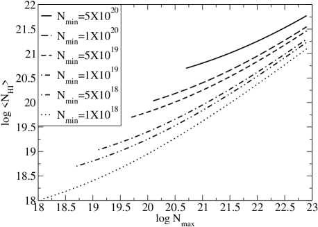
Figure 1: Values of the average column density $\langle N_{HI}\rangle$ are plotted versus central column density $N_{max}$, as in equation (2), for several values of limiting $N_{min}$. The curves are fairly flat for lower values of $N_{max}$. Thus fairly constant observed column densities would allow for $N_{max}$ to have a wide range of moderate to low values. The formula (2) plotted here is valid only for purely exponential discs, without considering ionization effects.

Some scatter is seen in the column density measurements from Minchin et al. (2003) and Rosenberg & Schneider (2003), and in central column densities found in studies of LSB galaxies such as de Blok, McGaugh, & van der Hulst (1996). Thus some variation is likely to occur for values of $N_{max}$, though its distribution is unknown.

Note that while the Rosenberg & Schneider (2003) data can be compared with the $\langle N_{HI}\rangle$ values shown above, Minchin et al. (2003) calculate column densities somewhat differently, so we will refer to these as ‘inferred’ column densities ($N_{HI}^{o}$) in order to distinguish from the averaged ones discussed above. In this case the complete HI mass of a galaxy is measured, assuming that the mass is entirely within the beam. Since they have not resolved their detected objects or obtained column density profiles, they use an estimate of the HI radius in order to find an inferred column density. They assume that the HI radii are equivalent to 5 times their observed effective optical radii, based upon the relationships from Salpeter & Hoffman (1996). Here we generally assume that such a radius corresponds to that where $N_{HI}=10^{20}$ cm^-2, although Salpeter & Hoffman (1996) base their relationships on several studies which may have slightly varying limiting values. Since the $N_{HI}^{o}$ values are found differently from $\langle N_{HI}\rangle$ values, they will depend here on what fraction of the HI mass is contained within the estimated radius. The inferred column density for an exponential disc where the complete mass is accurately measured would be

$$N_{HI}^{o}=\frac{N_{max}}{\ln^{2}(N_{max}/N_{min})}.$$ (3)

In this case $N_{min}$ is simply the column density corresponding to the estimated galaxy radius. Like equation (2), this formula does not depend upon the disc scale length.

Objects having $N_{max}\sim N_{min}$ will have more of their mass outside the radius at $N_{min}$, which will cause $N_{HI}^{o}$ to become large as seen in Fig. 2. Thus there is a minimum $N_{HI}^{o}$ value that can be detected for a given constant $N_{min}$. Objects having $N_{max}\sim N_{min}$ are likely to have small radii however, and these radii may be difficult to measure in a manner consistent with that used for larger objects. Thus an observer might effectively be using a smaller $N_{min}$ for a smaller $N_{max}$ when estimating any measurable radius for such an object. For example if $\log N_{min}=\log N_{max}-0.5$ then $N_{HI}^{o}=0.745N_{max}$ for an exponential disc, as shown by the dotted line in Fig. 2.

Different galaxy radii are used in different studies, inside of which the column densities are averaged or inferred. The data from Rosenberg & Schneider (2003) can be used to find averaged column densities for their sample out to a radius where $N_{HI}=2\times 10^{20}$ cm^-2, but their plotted HI masses and disc areas do not tell us about the properties of galaxies whose central column densities are about this value or lower. Based on their fit to the points in their first figure with a slope of one, their characteristic average column density would be $\langle N_{HI}\rangle^{*}=8.26\times 10^{20}$ cm^-2 or $10^{20.92}$ cm^-2, which would correspond to $N_{max}^{*}=10^{21.7}$ cm^-2 according to equation (2). However, points scattered within about half an order of magnitude of this value would suggest that galaxies exist that have $N_{max}$ values well below $10^{21}$ cm^-2. Many such objects are likely to have small HI radii above $2\times 10^{20}$ cm^-2, and thus need to be detected in a deeper survey such as that of Minchin et al. (2003).

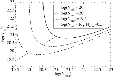
Figure 2: Values of inferred column density $N_{HI}^{o}$ are plotted versus central column density $N_{max}$, as in Equation (3), again for exponential discs without yet considering ionization, for several values of limiting $N_{min}$. Here the curves turn up for lower values of $N_{max}$ when a constant $N_{min}$ is assumed, as most of the mass will be outside the assumed radii for these objects. Thus there is a minimum $N_{HI}^{o}$ that can be measured for a given $N_{min}$, and lower $N_{HI}^{o}$ values can only be found if the radii are estimated differently for objects having low $N_{max}$ values, for example as shown in the line where $\log N_{min}=\log N_{max}-0.5$.

Minchin et al. (2003) report a characteristic $N_{HI}^{o*}=10^{20.6}$ cm^-2 for the HIDEEP sample. If we assume the $N_{max}^{*}$ value found above, then Equation (3) would give $N_{min}^{*}=10^{21.6}$ cm^-2, which would not allow for the detection of objects with very low, or even moderate, $N_{HI}^{o*}$. This $N_{min}^{*}$ value is probably too high to make sense or allow for the detection of many objects. However the HIDEEP survey is likely to detect objects with lower typical $N_{max}$ values than those of Rosenberg & Schneider (2003). Suppose we assume that the radii used by Minchin et al. (2003), who use five times the effective optical radii, are equivalent to those where $N_{min}\sim 10^{20}$ cm^-2 as is typical of the galaxies studied in Salpeter and Hoffman (1996). In this case, Equation (3) would give two solutions: $N_{max}^{*}=10^{21.9}$ cm^-2 and $N_{max}^{*}=10^{20.3}$ cm^-2, as seen in Fig. 2. The larger value would be unusually high compared to what is seen in galaxies with known HI profiles or damped absorbers, although the curve in Fig. 2 is not very steep for high $N_{max}$ values. On the other hand, objects having the lower $N_{max}$ value would likely have small radii so that the radii could be estimated less carefully than for larger objects. It is thus likely that objects with a wide range of $N_{max}$ values, including lower ones, are being detected by HIDEEP.

A larger radius, where $N_{min}<10^{20}$ cm^-2, would be needed to calculate $N_{HI}^{o}$ below $10^{20}$ cm^-2. However the limiting parameter for detecting clouds and galaxies in HI surveys is flux, rather than column density. Thus a more interesting question, as opposed to understanding the accuracy of galaxy radii, is whether objects having low values of $N_{max}$ and sizes or masses similar to those of known galaxies, could be detected in a survey having some limiting flux. We discuss this issue further using simulated galaxies in Sec. 4.

Note that column density profiles may fall off more slowly than exponentials in the outer parts of galaxies (Hoffman et al. 1993; see discussion in Linder et al. 2003). Furthermore, exponential profiles are not always well-behaved in the centres of galaxies where there may be stars or molecular gas instead of neutral hydrogen. (Thus $N_{max}$ becomes the extrapolated central column density assuming an exponential profile in the galaxy’s centre.) Finally, column density profiles are thought to fall off quickly at a few $\times 10^{19}$ cm^-2 due to ionization, which was not yet considered in Figs. 1 and 2. The effects of using more realistic column density profiles will be discussed further for simulated galaxies.

3 HI Profiles and Simulations

Simulations are done in order to determine the HI fluxes for possible populations of low column density objects, and to attempt to reproduce the distribution of inferred column densities seen in the HIDEEP survey. Samples of galaxies (or clouds, having unknown optical properties) are simulated at $z=0$ in order to produce the figures discussed in Section 4. Gas in each galaxy is modelled as a slab structure in hydrostatic equilibrium, where the gas is confined by a combination of pressure and gravity as in Charlton, Salpeter, & Hogan (1993) and Charlton, Salpeter & Linder (1994).

We wish to simulate objects having a wide range of properties, especially those which are low in mass or column density which may be difficult to detect due to ionization. We assume that each galaxy has an exponential total (neutral plus ionized) column density profile to start. Further simulations vary the profile, for example using a power law fall-off beyond four HI disc scale lengths, as discussed in Linder et al. (2003). The central (total) column density $N_{max}$ is assumed to have values which are uniformly distributed between $10^{18}$ and $10^{22.2}$ cm^-2. The higher central column density limit is chosen as an upper limit of what is seen in detected galaxies and damped Ly$\alpha$ absorbers, while the lower range is used in order to explore the possible existence of gas clouds which are more difficult to detect, being somewhat below the current sensitivity of HI surveys.

Disc scale lengths are chosen so that the simulated objects obey a Schechter-type total gas mass function, which gives rise to a detectable HI mass function having a similar slope of -1.3 (Zwaan et al. 2003) or -1.5 (Rosenberg & Schneider 2002). Two main cases are illustrated repeatedly in the following section: In Case A, we assume that the central column densities of the objects are correlated with the total gas masses. Case A is motivated by HI observations of LSB galaxies which suggest that they have lower central column densities (de Blok et al. 1996) and the likely existence of numerous dwarf LSB galaxies, such as in Sabatini et al. (2003). For each simulated galaxy a relationship is assumed for Case A where $\log N_{max}=21.7+1.0\log(M_{tot}-10.0)\pm 0.5$, so that objects having the lowest simulated $N_{max}$ values will tend to also have the gas masses around $10^{6}M_{\odot}$. (We later vary this relationship, as the narrow range of scatter is chosen as an extreme example to start.) In this case we have a substantial population of small clouds having low $N_{max}$, some of which might resemble HVCs, although the detectable objects will tend to have high $N_{max}$. In Case B the disc scale lengths and the central column densities are uncorrelated. Thus $N_{max}$ is uniformly distributed and unrelated to the total gas mass, but the scale lengths tend to be larger for objects having lower $N_{max}$. In this case we are simulating larger objects having low column densities, which might resemble giant LSB galaxies (whose numbers are very uncertain) or extended structures that give rise to Ly$\alpha$ absorption, as expected based upon double line of sight observations (for example, Dinshaw et al. 1998; Charlton, Churchill & Linder 1995; Monier, Turnshek & Hazard 1999; Fang et al. 1996).

Rotation velocities are found for each simulated galaxy using the relationships given in Salpeter & Hoffman (1996), where the Tully-Fisher relationship between the velocity $V_{rot}$ and the observable HI radius $R$ is found to be $V_{rot}/80.51~{}\mbox{km s}^{-1}=(R/12.3~{}\mbox{kpc})^{1.38}$. The value of $R$ is assumed to typically correspond to a radius where the limiting column density is $10^{20}$ cm^-2, but then this relationship does not give us information about the rotation velocities of massive objects having $N_{max}<10^{20}$ cm^-2. Since galaxies having a wide range of properties are found to obey a baryonic Tully-Fisher relation (McGaugh et al. 2000), we extrapolate the HI Tully-Fisher relation above into a baryonic version by assuming that $R$ in the formula above is the radius that a galaxy of equivalent (neutral plus ionized hydrogen) mass would have if it had $N_{max}=N_{max}^{*}$, where we assume $N_{max}^{*}=10^{21.7}$ cm^-2 as found in the previous section. When we attempt to simulate the smallest clouds, the value of $R$ may be very small, so that the velocity dispersion of the gas becomes more important. A minimum value of $V_{rot}=10$ km s^-1 is thus assumed. Note, however, that there is a selection effect against detecting objects having velocity widths $\mathrel{\raise 1.29167pt\hbox{$<$}\mkern-14.0mu\lower 2.58334pt\hbox{$\sim$}}50$ km s^-1 in HI surveys, as discussed in Minchin et al. (2003) and Lang et al. (2003).

The vertical ionization structure of the gas is modelled as in Linder (1998), which is similar to the model in Maloney (1993). Inside of some ionization radius $R_{cr}$, the gas is assumed to have a sandwich structure, where the inner shielded layer remains neutral and has a height ($z_{i}$) determined by equation (6) in Linder (1998). The gas above height ($z_{i}$) and beyond the ionization radius is assumed to be in ionization equilibrium.

The frequency- and direction-averaged ionization rate $\zeta$ is assumed at first to be $3.035\times 10^{-14}$ s^-1, from the calculation of Davé et al. (1999) at $z=0$ based upon spectra from Haardt & Madau (1996). The lowest measurements at redshifts $\sim 0$ tend to be consistent with this value as discussed in Linder et al. (2003). However galaxies, in addition to quasars, may contribute to the ionizing background radiation (Giallongo, Fontana, & Madau 1997; Shull et al. 1999; Bianchi, Cristiani, & Kim 2001; Linder et al. 2003). The ionizing intensity may be stronger when close to a luminous galaxy or galaxy-rich environment as shown in Linder et al. (2003), although the gas-rich objects which we are simulating here are not likely to arise in the most galaxy-rich environments. Thus simulations are also run using a larger frequency and direction-averaged ionizing intensity measurement for redshifts $z<1$ of $\zeta=1.9\times 10^{-13}$ s^-1 (Scott et al. 2002). The conversion between $\zeta$ and a one-sided flux is assumed as in Tumlinson et al. (1999). The radius $R_{cr}$, at which the disc becomes fully ionized, is found where the neutral gas height $z_{i}$ becomes zero.

For each galaxy, the neutral column density profile is calculated by integrating the neutral density $n_{HI}$ vertically through the disc, in increments of scale length $h/10$ (or smaller when needed for a more accurate mass calculation). The profiles have $N_{HI}\sim N_{tot}$ in the regions inside of $R_{cr}$. Just inside the radius $R_{cr}$, the column density falls off quickly, typically from $N_{HI}\sim 3\times 10^{19}$ cm^-2 to $N_{HI}\sim 10^{17}$ cm^-2, at which point the ‘ionized region’ of the disc is being mapped, and only a small fraction of the gas is neutral. The resulting profiles can then be integrated and averaged over suitable radii to be compared with HI observations.

In order to calculate fluxes for the simulated objects, each object is assigned a random inclination and a random distance within a sphere around us having a radius of 108 Mpc, the distance at which a $10^{10}M_{\odot}$ galaxy can be detected at a limiting peak HI flux of 18 mJy/beam, as in Minchin et al. (2003). The HI mass for each object, limited to what can be contained within a 15 arcmin beam centred on the galaxy, is binned into velocity channels of 15 km s^-1 when finding a peak or integrated flux, which is comparable to what is done for the HIDEEP survey.

4 Results

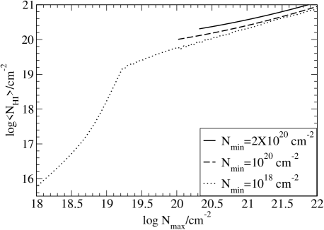
Figure 3: Averaged neutral column densities are plotted versus central neutral column densities ($N_{max}$) for simulated galaxies having exponential column density profiles with $h=2$ kpc which are exposed to an ionizing background. Column densities are found here by integrating HI masses out to $N_{min}$ and dividing by the area within the radius of $N_{min}$, where $N_{min}$ ranges from $2\times 10^{20}$ cm^-2 (top curve) to $10^{18}$ cm^-2 (bottom), which is indistinguishable from $N_{min}=10^{19}$ cm^-2 (for $N_{max}>10^{19}$ cm^-2) due to the steep column density profiles at these column densities resulting from ionization. The highest curve has $N_{min}$ equal to that in Rosenberg & Schneider (2003). The range of $\log\langle N_{HI}\rangle$ in this curve shown here is fairly narrow, thus showing that some variation is possible in $N_{max}$ for observed galaxies.

Averaged column densities are plotted, again versus central column density $N_{max}$, for simulated galaxies, which are exposed to an ionizing background. For simulated galaxies $N_{max}$ is defined as the total (neutral plus ionized) assumed central column density, which is about equal to the observable neutral value for $N_{max}>$ a few $\times 10^{19}$ cm^-2. For lower $N_{max}$ values, the neutral values could be as low as a few $\times 10^{17}$ cm^-2, although it is difficult to determine the value accurately very close to the centres of the discs with the model used here. Gas with column densities $\mathrel{\raise 1.29167pt\hbox{$<$}\mkern-14.0mu\lower 2.58334pt\hbox{$\sim$}}10^{19}$ cm^-2 are seen, for example as mini-HVCs (Hoffman et al. 2002).

Purely exponential total column density profiles are assumed for the objects simulated in Figs. 3 through 8. In Fig. 3, the column densities are averaged, so that the mass contained within a radius where $N_{HI}=N_{min}$ is divided by the area within this radius. Thus the right side of the plot looks similar to Fig. 1, but the left side shows where the averaged column densities become lower when most of the mass in a galaxy or HI cloud is close to the ionization edge.

Samples of 200 objects, having uniformly distributed values of $\log N_{max}$, are simulated in Figs. 3 and 4. We simulate only galaxies having $h=2$ kpc in Fig. 3, as the curve will otherwise become widened in the steeper parts ($N_{max}\mathrel{\raise 1.29167pt\hbox{$<$}\mkern-14.0mu\lower 2.58334pt\hbox{$\sim$}}10^{20}$ cm^-2) due to variations in disc scale lengths. The top curve shows objects observed to the same limits as in Rosenberg & Schneider (2003). It can be seen that less than one order of magnitude of variation in $\langle N_{HI}\rangle$ corresponds to more than two orders of magnitude in possible $N_{max}$ values.

In Fig. 4 we plot inferred column densities ($N_{HI}^{o}$), also versus central column density $N_{max}$, for simulated objects which are exposed to an ionizing background. Inferred column densities are found by dividing the total HI mass of a galaxy or cloud by an area within some estimated HI radius. One might use a radius where ($N_{min}\sim 10^{20}$ cm^-2) which would be typical of the galaxies discussed in Salpeter and Hoffman (1996), but it would be necessary to use a radius corresponding to a smaller $N_{min}$ to find a smaller $N_{HI}^{o}$. Thus we assume here (and for further calculations of $N_{HI}^{o}$) that $N_{min}=10^{20}$ cm^-2 or that $\log N_{min}=\log N_{max}-0.5$ if $\log N_{min}<20.5$. In Fig. 4 we show several scale length values between 0.2 and 4 kpc. The upper parts of the curves (having $\log N_{max}>20.5$) are similar to the central curve in Fig. 2, although any variation with $h$ happens only with an ionizing background. Here the lower curves, where $\log N_{min}=\log N_{max}-0.5$ are steepened due to ionization, when compared to the line with slope 0.745 without ionization.

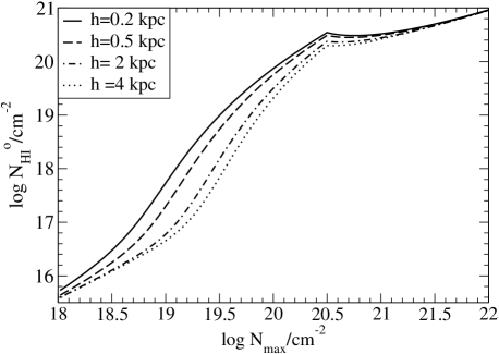
Figure 4: Inferred neutral column densities are plotted versus central neutral column densities ($N_{max}$) for simulated galaxies which are exposed to an ionizing background. Column densities are found here by dividing total HI masses by the area within the radius of $N_{min}$, where $N_{min}=10^{20}$ cm^-2 or that $\log N_{min}=\log N_{max}-0.5$ if $\log N_{min}<20.5$. Curves are shown for several disc scale length values, ranging from $0.2$ to 4 kpc. Note that the curves are much steeper at low $N_{max}$ than the line shown in Fig. 2 due to ionization.

It can be seen in Figs. 3 and 4 that the averaged and inferred column densities both fall off quickly when $N_{max}$ goes below some value $\mathrel{\raise 1.29167pt\hbox{$<$}\mkern-14.0mu\lower 2.58334pt\hbox{$\sim$}}10^{20}$ cm^-2, though the $N_{HI}^{o}$ or $\langle N_{HI}\rangle$ value where this happens depends upon the assumed value of $N_{min}$. The steepening of the dotted curve in Fig. 3 is a result of galaxy discs having ionization edges at a few $\times 10^{19}$ cm^-2. For the inferred column densities shown in Fig. 4 the steepening happens in part because of the radius withinin which the column density is averaged, as it is for the dotted line shown in Fig. 2. However, the line in Fig. 2 has a slope of 0.745, whereas in Fig.4, $N_{HI}^{o}$ changes by about four orders of magnitude when $N_{max}$ changes by two orders of magnitude, which is as steep as a line with a slope of $2$, again resulting from ionization. For objects having low $N_{max}$, the area of the disc which has a high column density becomes small, so that the HI fluxes for these objects are also likely to be small.

While $N_{HI}^{o}$ values may difficult to estimate, we ultimately want to know which central column density $N_{max}$ values can be detected in a survey having some limiting flux. In Figs. 5 through 8, we plot peak fluxes for simulated galaxies, which can be compared with the HIDEEP limiting value of 18 mJy per velocity channel, where the velocity resolution is 18 km/s and the channel separation is 13.2 km/s. corresponding to the vertical line in each Figure. Samples of 5000 objects, having total gas masses between $10^{6}$ and $10^{11}$ $M_{\odot}$ which obey a total gas mass function with a slope of -1.3, are simulated for each case.

In Fig. 5, central column density values are plotted versus peak flux values which would be produced by completely unionized gas. More objects have lower fluxes than higher ones at any given $N_{max}$, as there are more objects which are at larger distances, and more having lower masses. In Case A (black circles), where the simulated masses are correlated with $N_{max}$, and thus low $N_{max}$ objects tend to have smaller scale lengths, an observer would not expect to detect many objects having $N_{max}\mathrel{\raise 1.29167pt\hbox{$<$}\mkern-14.0mu\lower 2.58334pt\hbox{$\sim$}}10^{20}$ cm^-2, even without considering the effects of ionization. Yet if the objects with low $N_{max}$ are as massive as those having high $N_{max}$ (Case B, grey circles), then numerous objects having low $N_{max}$ would still be seen above a reasonable flux limit. The fluxes for objects having lower $N_{max}$ values would only be lower if a substantial fraction of the mass is outside the beam, as seen for $N_{max}\mathrel{\raise 1.29167pt\hbox{$<$}\mkern-14.0mu\lower 2.58334pt\hbox{$\sim$}}10^{19}$ cm^-2, or if some of the gas is ionized, as seen in Fig. 6. In Fig. 6, values of $N_{max}$ are plotted versus peak flux for each object, now including the effects of ionization. At a limiting flux above that in the HIDEEP survey, few objects could be detected having $N_{max}>10^{20}$ cm^-2 (although the detectable inferred column densities could be lower than this value, as seen in Fig.  8). It can be seen that an observer would need to look at least two orders of magnitude fainter than the HIDEEP limit to detect ionized objects having $N_{max}\mathrel{\raise 1.29167pt\hbox{$<$}\mkern-14.0mu\lower 2.58334pt\hbox{$\sim$}}10^{20}$ cm^-2 in Case B, or possibly more if low column density objects are less massive. The fluxes shown, for example, for ionized objects here, may be lower limits if the gas far from galaxies is clumpy.

In Figs. 7 and 8, we attempt to calculate inferred column densities, which are plotted again versus peak flux, and can be compared with the $N_{HI}^{o}$ values for the HIDEEP survey. Again we find $N_{HI}^{o}$ values within radii where $\log N_{min}=20$ or $\log N_{min}=\log N_{max}-0.5$ if $\log N_{max}<20.5$, which makes sense, as all the objects detected in HIDEEP were found to have possible optical counterparts, and are thus assumed to have measurable HI radii. In Fig. 7 we show the total inferred column densities ($N_{tot}^{o}$), or the neutral gas that would be seen if there were no ionizing background. A flat distribution of $N_{max}$ values has been assumed all along for Case B, while even more objects with low $N_{max}$ are simulated in Case A, yet the majority of the points which are above the limiting flux are seen at $N_{tot}^{o}\sim 10^{20.6}$ cm^-2. Thus the $N_{HI}^{o}$ values found in HIDEEP, where the distribution is peaked at $10^{20.65}$ cm^-2, should have a strongly peaked distribution simply as a result of averaging exponential profiles over a radius where $N_{min}=10^{20}$ cm^-2. Yet numerous lower $N_{tot}^{o}$ would still be seen, especially for Case B.

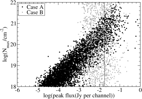
Figure 5: Without an ionizing background, central column densities $N_{max}$ are plotted versus peak fluxes for simulated galaxies having purely exponential profiles, both for a sample of objects where the HI masses are correlated with $N_{max}$ (Case A, black circles) and for a sample where the masses are independent of central value $N_{max}$ (Case B, grey circles). A line is drawn at the limiting flux of the HIDEEP survey. If the lower column density galaxies were unionized, as shown here, galaxies having a wider range of central column densities would be detectable.

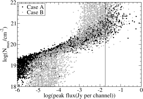
Figure 6: Central column density ($N_{max}$) values are plotted versus peak fluxes for simulated galaxies, for the cases shown in Fig. 5, but now exposed to an ionizing background. Few points having $N_{max}$ below $10^{20}$ cm^-2 can be detected below the limiting flux of the HIDEEP survey.

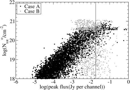
Figure 7: Inferred column density values ($N_{tot}^{o}$), without an ionizing background are plotted versus peak fluxes for simulated galaxies, again for the cases described in Fig. 5, assuming radii where $\log N_{min}=20$ or $\log N_{min}=\log N_{max}-0.5$ if $\log N_{max}<20.5$. The majority of the points, which are above the HIDEEP limiting flux, are seen at $10^{20.6}$ cm^-2. Some lower $N_{tot}^{o}$ values could be detected, in this hypothetical unionized case, if the radii of these objects were correctly estimated.

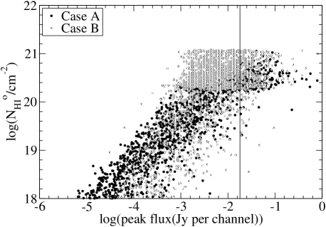
Figure 8: Inferred column density ($N_{HI}^{o}$) values are plotted versus peak fluxes for simulated galaxies, for the two cases described in Fig. 5 Here the gas has been exposed to an ionizing background, and $N_{min}$ values are assumed as in Fig. 7 Above the limiting HIDEEP flux, only a few points might be detected having $N_{max}\mathrel{\raise 1.29167pt\hbox{$<$}\mkern-14.0mu\lower 2.58334pt\hbox{$\sim$}}10^{20}$ cm^-2.

The $N_{HI}^{o}$ values, as seen when the gas is exposed to an ionizing background, are shown in Fig. 8. Here only a few galaxies or clouds having $N_{HI}^{o}<10^{20}$ cm^-2 are seen above the HIDEEP flux limit. In either of the cases, it should be possible to detect more objects having low $N_{HI}^{o}$ in a survey which is just slightly deeper than HIDEEP, if the radii of the objects can be estimated accurately enough. For Case A the objects shown appear to have a similar relationship between peak flux and column density as in the unionized plot, but the main difference is that more of the objects have inferred column densities that are below the minimum value shown on the plot. Here the distribution of detectable $N_{HI}^{o}$ values appears to be somewhat less strongly peaked compared to the unionized cases, yet the binned points, which are simulated like those above the HIDEEP flux limit in Fig. 8, do not look very different from the HIDEEP distribution, as shown in Figs. 9 and 10.

In Figs. 9 and 10 we show the inferred column density distributions for Cases A and B respectively, for samples of $1000$ objects having peak fluxes $>18$ mJy and velocity widths $>40$ km/s. Also shown is the Gaussian curve fitted to the HIDEEP galaxies, having a mean of 20.65 and a scatter of 0.38, as in Minchin et al. (2003) and the binned data from Minchin et al. (2003). Neither histogram is very different from the Gaussian or data set, assuming some measurement uncertainties. Case A appears to be somewhat strongly peaked here, although the observational uncertainties, mostly in measuring the area of the galaxies, are not yet shown here. Case B appears to be more broad, and similar to the plotted Gaussian. The peak feature at $10^{20.3}$ cm^-2 is also seen in the Minchin et al. (2003) data. This feature is a result of many galaxies with high $N_{max}$ having their column densities averaged over similar $N_{min}$, and confirms that similar galaxy radii are being used to find the inferred column densities for the majority of the galaxies for the observations and for the simulations done here. The Case A model looks more realistic at the high column density end of the distribution, although we do not model high column density galaxies carefully given that more of their gas may be converted into stars or ionized by these stars. Neither distribution is very different from the Gaussian curve, although the most realistic scenario is likely to have an intermediate behaviour between Cases A and B. There is likely to be some relationship between the gas masses and central column densities of galaxies, but the scatter may be larger than we have assumed in Case A. For example, we increase the amount of scatter for $N_{max}$ from 0.5 to 1.5 orders of magnitude in Case C.

In Case B (Fig. 10) there are a few objects seen which have sufficiently high fluxes to be detected, but column densities below anything detected by HIDEEP. (These points are not seen for Case A, only because sufficiently low column densities are assumed to arise only in very low mass galaxies which are all below the HIDEEP flux limit.) Such points may have simply not yet been detected by HIDEEP due to the small number of objects detected, compared to the 1000 objects simulated here. Also, these objects may have small, and thus uncertain radii. Very few HI clouds are thought to have no optical counterparts (Davies et al. 2004), and there are no clouds detected which have no optical counterparts in HIDEEP. This could happen because the gas is actually more clumpy than we have modelled here, so that star formation occurs in small regions within these clouds. The isolated HI cloud detected by Giovanelli & Haynes (1989), for example, was later found by many observers to contain a small dwarf galaxy. The radii for such objects are thus likely to be underestimated, so that their inferred column densities will be higher than what we find here.

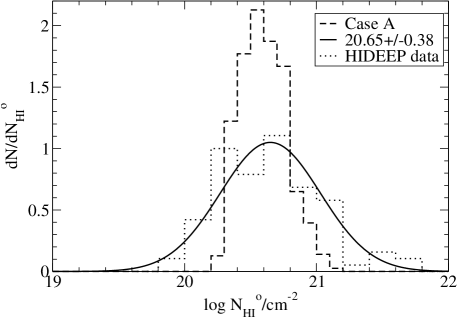
Figure 9: Distributions are shown for simulated inferred column density ($N_{HI}^{o}$) values detected above the limiting flux of HIDEEP, for Case A, where the gas mass for each galaxy is closely related to $N_{max}$ (dashed line). Also shown is the Gaussian curve fitted to the HIDEEP sample (solid line) and the binned HIDEEP data (dotted line).

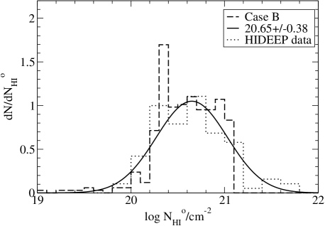
Figure 10: Distributions are shown for simulated $N_{HI}^{o}$ values detected above the limiting flux of HIDEEP, for Case B, where the total gas mass is independent of $N_{max}$ (dashed line). Also shown is the Gaussian curve fitted to the HIDEEP sample (solid line) and the binned HIDEEP data (dotted line).

The inferred column density distributions for the unionized cases are surprisingly indistinguishable from those shown in Figs. 9 and 10, when assuming that galaxies having velocity widths $<40$ km/s are not detectable, although these objects were not removed from Figs.  5 through 8. Thus velocity width related selection effects could be as important as ionization in determining the shape of the distribution of inferred column densities. Objects which could be ionized to the point of being undetectable have low masses and thus low velocity widths in Case A. In Case B the distribution of $N_{HI}^{o}$ is the same for detected and undetected objects. However the neutral and ionized column density distributions are not the same in the intermediate Case C, where $\log N_{max}=21.7+1.0\log(M_{tot}-10.0)\pm 1.5$, as some galaxies having detectable velocity widths are affected by ionization, yet there is some variation with galaxy mass. In Case C the $N_{tot}^{o}$ distribution is very strongly peaked, yet the $N_{HI}^{o}$ distribution is somewhat broad, and similar to that seen for Case B.

The biggest source of uncertainty in finding inferred column densities is in measuring the galaxy radii. When an uncertainty of $40\%$ in the radii is included, as shown in Fig. 11, Case A is still too strongly peaked, while Cases B and C are more similar to each other and to the Gaussian curve fitted to the HIDEEP data. Fluctuations in the ionizing background radiation are also likely to broaden the distributions somewhat, but only by increasing the number of galaxies with high $N_{HI}^{o}$ as there are few locations in space (Linder et al. 2003) where the ionizing background is as low as the value assumed here (Haardt & Madau 1996).

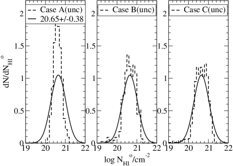
Figure 11: Distributions of simulated $N_{HI}^{o}$ (dashed lines) are shown with uncertainty in the measured galaxy radii included for Cases A (left), B (centre), and C (right). Also shown is the Gaussian curve fitted to the HIDEEP sample in each frame (solid line).

A summary of the simulations is given in Table 1, where the mean and scatter values for the $N_{HI}^{o}$ distributions are listed. Case C is intended to be intermediate between the Cases A and B shown previously, as there is some correlation between $N_{max}$ and the gas masses, but a larger scatter so that $\log N_{max}=21.7+1.0\log(M_{tot}-10.0)\pm 1.5$.

In an attempt to put some constraints on the properties of the objects detected in the HIDEEP survey, some further variations were made of the model parameters. The slope in the $\log N_{max}$–$\log M_{tot}$ relationship was increased from $1.0$ to $1.2$, which resulted in a strongly peaked inferred column density distribution similar to that for Case A. In further simulations we assume that $\log N_{max}=21.7+1.0\log(M_{tot}-10.0)\pm 1.5$ as in Case C. Flattening the central parts of the galaxy column density profiles (to a value between $10^{20.5}$ and $10^{21.5}$ cm^-2) also gave rise to a strongly peaked distribution as in Case A. We also simulated a stronger ionizing background, based upon the $z<1$ measurements of Scott et al. (2002), and did a simulation using a steeper slope of $-1.5$ for the HI mass function, as reported by Rosenberg & Schneider (2002). In both of these cases the inferred column distribution is similar to that in Case C. Furthermore we varied the characteristic $N_{max}$ value, so that $\log N_{max}=22.2+1.0\log(M_{tot}-10.0)\pm 1.5$ while using flattened central column density profiles in order to allow for higher extrapolated $N_{max}$ values as suggested in Bowen, Blades, & Pettini (1996). In this case the $N_{HI}^{o}$ distribution is somewhat strongly peaked. A further simulation was done where the exponential column density profiles were flattened to a power law with a slope of $-4$ beyond four HI scale lengths, in which case we see a slightly excessive number of high column density galaxies. Combining the slow fall-off in the outer parts with a reduced central column densities would likely give rise to a more realistic number of high column density galaxies. For any of the parameter variations, the distribution is not very different from the Gaussian curve fitted to the HIDEEP points, given the uncertainty in the actual relationship between gas masses and central column densities.

Table 1: Inferred Column Densities and Lyman Limit Absorber Counts

Case	$\langle\log N_{HI}^{o}\rangle$	$\sigma(\log N_{HI}^{o})$	$(dN/dz)_{0,LL}$
A	20.65	0.22	2.61
B	20.62	0.30	0.93
C	20.63	0.30	1.22
Au	20.61	0.20
Bu	20.63	0.33
Cu	20.61	0.32

Mean inferred column densities, scatter for the inferred column density distributions, and Lyman limit absorber counts are shown for the simulations as summarized here:
Case A, where gas masses are related to $N_{max}$ such that $\log N_{max}=21.7+1.0\log(M_{tot}-10.0)\pm 0.5$;
Case B, where gas masses are independent of $N_{max}$;
Case C, where $\log N_{max}=21.7+1.0\log(M_{tot}-10.0)\pm 1.5$;
Cases Au, Bu, and Cu, versions including uncertainties in galaxy radii.

5 Lyman limit absorber counts

Lyman limit absorber counts, arising from quasar lines of sight through gas having $10^{17.2}<N_{HI}<10^{20.3}$ cm^-2 provide further constraints on the numbers and properties of undetected objects containing low column density gas. Estimates have been made for the number of Lyman limit systems arising in optically observed galaxies, but this generally involves assuming a cross section for absorption around a galaxy as a function of its optical luminosity (Linder et al. 2003; Steidel 1995; Bergeron & Boissé 1991). However the relationship between optical and HI properties of galaxies may not be well enough understood to make such estimates. Here we can estimate the number of Lyman limit systems arising from galaxies that obey an observed HI mass function instead.

We estimate the number of Lyman limit systems arising in each scenario by putting random lines of sight through the sphere in which the galaxies are simulated and finding the column density where a line of sight intersects a galaxy. We simulate 20,000 galaxies in an eighth of a sphere having a radius of 108 Mpc, and use 10,000 lines of sight for each case. The number of Lyman limit systems is then calculated by correcting to a number density of simulated objects which gives rise to an HI mass function having a normalization consistent with Zwaan et al. (1997). The minimum galaxy mass of $10^{7}M_{\odot}$ is used for simulated galaxies, as the lowest mass objects are not likely to make a substantial contribution to Lyman limit (or lower column density) absorber counts (Linder 1998), although estimates from HI studies suggest that slightly more massive objects do contribute to Lyman limit absorption (Ryan-Weber et al. 2003). Values for the number of Lyman limit absorbers per unit redshift along a line of sight, $(dN/dz)_{0,LL}$, are shown for the three main simulations in Table 1.

The number of Lyman limit absorbers has been measured at redshifts $\geq 0.36$, and the evolution is seen to be about flat or slightly decreasing down to redshift zero. The lowest redshift values available are within the range of $(dN/dz)_{LL}\sim 0.2$ to 1.3 (Lanzetta, Wolfe, & Turnshek 1995b; Storrie-Lombardi et al. 1994; Stengler-Larrea et al. 1995). Most of the simulations appear to be consistent with these observations, although Case A gives rise to too many absorbers. The simulation where the ionizing background intensity was increased gives rise to too few (0.08) absorbers per unit redshift, but the ionizing intensity used is probably more relevant at $z\sim 1$, where there are actually more absorbers because less cosmological expansion has occurred.

Case A (and some other simulations giving more strongly peaked $N_{HI}^{0}$ distributions) appear to give rise to a somewhat excessive numbers of Lyman limit systems. However, the same problem seems to arise when estimating the number of Lyman limit systems around galaxies whose optical luminosity function is known. It has long been thought that luminous galaxies have sufficient cross sections to explain the Lyman limit absorber counts fully, yet it is not known why dwarf and LSB galaxies would not also make some contribution, especially now that such faint objects are often found to give rise to damped Ly$\alpha$ absorption. It is possible, for example, that feedback processes change the column density profiles in the outer parts of some galaxies (McLin, Giroux, & Stocke 1998). While we do not rule out cases simply because they give rise to somewhat excessive Lyman limit absorber counts, Case A also has an excessively peaked distribution of inferred column densities, which is not improved when taking uncertainties in measuring the galaxy radii into consideration. Thus allowing for a wider range of galaxy column density profiles could make Lyman limit absorber counts more consistent with what we expect from observed galaxies.

6 Conclusions

Most galaxies have inferred column densities around $10^{20.6\pm 0.3}$ cm^-2 because inferred column densities are found by averaging column density profiles, which are exponential or similar, over a radius where the minimum column density is $\sim 10^{20}$ cm^-2. Ionization plays some role in making lower column density objects undetectable, including those without substantial optical counterparts. However inferred column density distributions tell us little about the distribution of central column densities in galaxies and clouds.

Ionization by the background of ultraviolet photons will strongly affect the amount of neutral gas remaining, and thus the HI flux detected, in objects having low hydrogen column densities, if such objects having sizes comparable to galaxies exist. Typical HI fluxes are reduced, as a result of ionization, by a factor of $\sim 100$ for galaxies having peak column densities $N_{max}\sim 10^{19.5}$ cm^-2 compared to those with $N_{max}\sim 10^{20}$ cm^-2, even if the lower column density galaxies are extended in size and just as massive as the higher column density galaxies.

We do not always know the central column densities of the faintest HI sources, but the detected inferred column densities are also likely to be above $\sim 10^{20}$ cm^-2 for most observable galaxies. Inferred column densities are rather weakly related to central column densities for objects having exponential profiles. Furthermore, since HI profiles tend to be mapped out to limiting column densities $\sim 10^{20}$ cm^-2, it may be difficult to estimate the radii, and thus the inferred column densities in a consistent manner for objects having lower $N_{max}$ values. For example, if the radii are underestimated, which might be more likely to happen for an extended, diffuse galaxy, the inferred column density could be overestimated. Other selection effects, such as those against objects having low velocity widths, may also be important in understanding the observed distribution of inferred HI column densities.

The observed distribution of inferred HI column densities, as seen by Minchin et al. (2003), can easily be simulated assuming possible populations of galaxies having a wide range of size and central column density distributions, and the simulated distributions are similar to the HIDEEP distribution for a wide range of model parameters. (Thus the ’Frozen Disc’ hypothesis of Minchin et al. 2003 seems to be unnecessary in explaining these observations.) However, we are thus given little constraint on the properties of gas rich objects which have so far escaped detection in the deepest HI surveys. Given the effects of ionization, we are unable to rule out the existence of undetected populations of very faint dwarf galaxies or giant gas clouds, as long as they have low central column densities. Such objects could make some contribution to Ly$\alpha$ absorption, although a more reasonable number of Lyman limit systems arises if galaxies have a wide, rather than narrow, range of central column densities.

The ionizing background radiation is more intense at redshifts around 1 or 2 than at redshift zero (Haardt & Madau 1996), and therefore some of the apparently younger galaxies, such as LSB galaxies, may have been ionized at these redshifts if they have lower central column densities (de Blok et al. 1996), thus slowing their evolution. Ionization may have also affected the formation of dwarf galaxies in certain environments at high redshifts (Efstathiou 1992; Tully et al. 2002), as less dense environments are more likely to be optically thin to ionizing radiation when the dwarf galaxies formed. Thus dwarf galaxies may have formed more easily in rich clusters such as Virgo (Sabatini et al. 2003) and Fornax (Kambas et al. 2000) than in more diffuse clusters such as Ursa Major (Trentham & Tully 2002) and other environments (Roberts et al. 2003). Understanding the role that ionization plays is thus important in testing Cold Dark Matter scenarios and other theories related to galaxy formation.

References

- Bahcall (1996) Bahcall, J. N. et al. 1996, ApJ, 457, 19
- Bergeron (1991) Bergeron, J., & Boissé, P. 1991, A&A, 243, 344
- Bianchi (1991) Bianchi, S., Cristiani, S., & Kim, T.-S. 2001, A&A, 376, 1
- Bland-Hawthorna (1994) Bland-Hawthorn, J., Taylor, K., Veilleux, S. & Shopbell, P. L. 1994, ApJ, 437, L95
- Bland-Hawthornb (1998) Bland-Hawthorn, J. 1998, in D. Zaritsky, ed., Galaxy Halos, ASP Conf. Ser. 136, San Francisco, p. 113
- Bland-Hawthornc (1997) Bland-Hawthorn, J., Freeman, K. C., & Quinn, P. J. 1997, ApJ, 490, 143
- Blitz (1999) Blitz, L., Spergel, D. N., Teuben, P. J., Hartmann, D., & Burton, W. B. 1999, ApJ, 514, 818
- Bochkarev (1977) Bochkarev, N. G. & Sunyaev, R. A. 1977, Soviet Astr., 21, 542
- Bowena (1996) Bowen, D. V., Blades, J. C., & Pettini, M. 1996, ApJ, 448, 662
- Bowenb (2001) Bowen, D. V. Tripp, T. M., & Jenkins, E. B. 2001, AJ, 121, 1456
- Charltona (1993) Charlton, J. C., Salpeter, E. E., & Hogan, C. J. 1993, ApJ, 402, 493
- Charltonb (1994) Charlton, J. C., Salpeter, E. E., & Linder, S. M. 1994, ApJ, 430, L29
- Charltonc (1995) Charlton, J. C., Churchill, C. W., & Linder, S. M. 1995, ApJ, 452, L81
- Charltond (2000) Charlton, J. C., Churchill, C. W., & Rigby, J. R. 2000, ApJ, 544, 702
- Chen (2001) Chen, H. -W., Lanzetta, K. M., Webb, J. K., Barcons, X. 2001, ApJ, 559, 654
- Cohen (2001) Cohen, J. G. 2001, AJ, 121, 1275
- Corbelli (1993) Corbelli, E. & Salpeter, E. E. 1993, ApJ, 419, 104
- Dahlem (2001) Dahlem, M., Ehle, M., & Ryder, S. D. 2001, A&A, 473, 85
- Davé (1999) Davé, R., Hernquist, L., Katz, N., & Weinberg, D. H. 1999, ApJ, 511, 521
- Daviesa (2001) Davies, J. I., de Blok, W. J. G., Smith, R. M., Kambas, A., Sabatini, S., Linder, S. M., & Salehi-Reyhani, S. A. 2001, MNRAS, 328, 1151
- Daviesb (2002) Davies, J., Sabatini, S., Davies, L., Linder, S., Roberts, S., Smith, R., & Evans, Rh. 2002, MNRAS, 336, 155
- Daviesc (2004) Davies, J. et al. 2004, MNRAS, 349, 922
- de Bloka (1996) de Blok, W. J. G., McGaugh, S. S., & van der Hulst, J. M. 1996, MNRAS, 283, 18
- de Blokb (2002) de Blok, W. J. G., Zwaan, M. A., Dijkstra, M., Briggs, F. H., & Freeman, K. C. 2002, A&A, 382, 43
- Dinshaw (1998) Dinshaw, N., Foltz, C. B., Impey, C. D., & Weymann, R. J. 1998, ApJ, 494, 567
- Dove (1994) Dove, J. B. & Shull, J. M. 1994a, ApJ, 423, 196
- Efstathiou (1992) Efstathiou, G. 1992, MNRAS, 256, 43
- Fang (1996) Fang, Y., Duncan, R. C., Crotts, A. P. S., Bechtold, J. 1996, ApJ, 462, 77
- Giallongo (1997) Giallongo, E., Fontana, A., & Madau, P. 1997, MNRAS, 289, 629
- Giovanellia (1983) Giovanelli, R. & Haynes, M. P. 1983, AJ, 88, 881
- Giovanellib (1989) Giovanelli, R. & Haynes, M. P. 1989, ApJ, 346, 5
- Haardt (1996) Haardt, F. & Madau, P. 1996, ApJ, 461, 20
- Haynes (1984) Haynes, M. P. & Giovanelli, R. 1984, AJ, 89, 158
- Hoffmana (1993) Hoffman, G. L., Lu, N. Y., Salpeter, E. E., Farhat, B., Lamphier, B., & Roos, T. 1993, AJ, 106, 39
- Hoffmanb (2002) Hoffman, G. L., Salpeter, E. E., & Pocceschi, M. G. 2002, ApJ, 576, 232
- Kambas (2000) Kambas, A., Davies, J. I., Smith, R. M., Bianchi, S., & Haynes, J. A. 2000, AJ, 120, 3
- Klypin (1999) Klypin, A. A., Kravtsov, A. V., Valenzeula, O. & Prada, F. 1999, ApJ, 522, 82
- Lang (2003) Lang, R. H., Boyce, P. J., Kilborn, V. A., Minchin, R. F., Disney, M. J., Jordan, C. A., Grossi, M., Garcia, D. A., Freeman, K. C., Phillipps, S., & Wright, A. E. 2003, MNRAS, 342, 738
- Lanzetta (1995) Lanzetta, K. M., Wolfe, A. M., & Turnshek. D. A. 1995, ApJ, 440, 435
- Lindera (1998) Linder, S. M. 1998, ApJ, 495, 637
- Linderb (2000) Linder, S. M. 2000, ApJ, 529, 644
- Linderc (2003) Linder, S. M., Gunesch R., Davies, J. I., Baes, M., Evans, Rh., Roberts, S., Sabatini, S., & Smith, R. 2003, MNRAS, 342, 1093
- Maloney (1993) Maloney, P. 1993, ApJ, 414, 41
- McGaugh (2000) McGaugh, S. S., Schombert, J. M., Bothun, G. D., de Blok, W. J. G. 2000, ApJ, 533, 99
- McLin (1998) McLin, K. M., Giroux, M. L., & Stocke, J. T. 1998, in D. Zaritsky, ed., Galaxy Halos, ASP Conf. Ser. 136, San Francisco, p. 175
- Minchina (2001) Minchin, R. F. 2001, PhD Thesis, Cardiff University
- Minchinb (2003) Minchin, R. F. et al. 2003, MNRAS, 346, 787
- Monier (1999) Monier, E. M., Turnshek, D. A., & Hazard, C. 1999, ApJ, 522, 627
- Moore (1999) Moore, B. Ghigna, S., Governato, F., Lake, G., Quinn, T., Stadel, J., & Tozzi, P. 1999, ApJ, 524, L19
- Rigby (2002) Rigby, J. R., Charlton, J. C., & Churchill, C. W. 2002, ApJ. 565, 743
- Roberts (2002) Roberts, S., Sabatini, S., Davies, J., Baes, M., Linder, S., Smith, R. & Evans, Rh. 2003, MNRAS, in press
- Rosenberga (2003) Rosenberg, J. L., & Schneider S. E. 2003, ApJ, 585, 256
- Rosenbergb (2002) Rosenberg, J. L., & Schneider S. E. 2002, ApJ, 567, 247
- Ryan-Weber (2003) Ryan-Weber, E. V., Webster, R. L., & Staveley-Smith, L. 2003, MNRAS, 343, 1195
- Sabatini (2003) Sabatini, S., Davies, J., Scaramella, R., Smith, R., Baes, M., Linder, S. M., Roberts, S., & Testa, V. 2003, MNRAS, 341, 981
- Salpeter (1996) Salpeter, E. E., & Hoffman, G. L. 1996, ApJ, 465, 595
- Scott (2002) Scott, J., Bechtold, J., Morita, M., Dobrzycki, A., & Kulkarni, V. 2002, ApJ, 571, 665
- Shull (1999) Shull, J. M., Roberts, D., Giroux, M. L., Penton, S. V., & Fardal, M. A. 1999, AJ, 118, 1450
- Steidel (1995) Steidel, C. C. 1995, in G. Meylan, ed., QSO Absorption Lines, Springer–Verlag, Berlin, p. 139
- Stengler-Larrea (1995) Stengler-Larrea et al. 1995, ApJ, 444, 64
- Stocke (1995) Stocke, J. T., Shull, J. M., Penton, S., Donahue, M., Carilli, C., 1995, ApJ, 451, 24
- Storrie-Lombardi (1994) Storrie-Lombardi, L. J., McMahon, R. G., Irwin, M. J., & Hazard, C. 1994, ApJ, 427, L13
- Swaters (2002) Swaters, R.A., van Albada, T.S., van der Hulst, J.M., & Sancisi, R. 2002, A&A, 390, 829
- Thilker (2004) Thilker, D. A., Braun, R., Walterbos, R. A. M., Corbelli, E., Lockman, F. J., Murphy, E., & Maddalena, R. 2004, ApJ, 601,39
- Trentham (2002) Trentham, N. & Tully, R. B. 2002, MNRAS, 335, 3
- Tully (2002) Tully, R. B., Somerville, R. S., Trentham, N., & Verheijen, M. A. W. 2002, ApJ, 569, 573
- Tumlinson (1999) Tumlinson, J., Giroux, M. L., Shull, J. M., & Stocke, J. T. 1999, AJ, 118, 2148
- Turnshek (2000) Turnshek, D. A., Rao, S., Nestor, D., Lane, W., Monier, E., Bergeron, J., Smette, A. 2000, ApJ, 553, 288
- Verheijena (2001) Verheijen, M. A. W. & Sancisi, R. 2001, A&A, 370, 765
- Verheijenb (2000) Verheijen, M. A. W., Trentham, N., Tully, R. B., & Zwaan, M. A. 2000, in Mapping the Hidden Universe in HI, et. R. C. Kraan- Korteweg, P. A. Henning, & H. Andernach, ASP Conf. Ser. 218, 263
- Watson (1984) Watson, W.D. & Deguchi, S. 1984, ApJ, 281, L5
- Zwaana (2003) Zwaan, M. A. et al. 2003, AJ, 125, 2842
- Zwaanb (2001) Zwaan, M. A. 2001, MNRAS, 345, 1142
- Zwaanc (2000) Zwaan, M. A. & Briggs, F. H. 2000, ApJ, 530, L61
- Zwaand (1997) Zwaan, M. A., Briggs, F. H., Sprayberry, D. & Sorar, E. 1997, ApJ, 490, 173