Affleck-Dine Baryogenesis and Heavy Element Production from Inhomogeneous Big Bang Nucleosynthesis

Abstract

Recent observations have revealed that small-scale structure exists at high redshift. We study the possibility of the formation of such structure during baryogenesis and big bang nucleosynthesis. It is known that under certain conditions, high density baryonic bubbles are created in the Affleck-Dine model of baryogenesis, and these bubbles may occupy a relatively small fraction of space, while the dominant part of the cosmological volume is characterized by the normal observed baryon-to-photon ratio, $\eta=6\cdot 10^{-10}$. The value of $\eta$ in the bubbles could be much larger than the usually accepted value (indeed, even close to unity) and still be consistent with the existing data on light element abundances and the observed angular spectrum of cosmic microwave background radiation (CMBR). We find upper bounds on $\eta$ by comparing the abundances of heavy elements produced in big bang nucleosynthesis (BBN) and those of metal poor stars. We conclude that $\eta$ should be smaller than $10^{-5}$ in some metal poor star regions.

1 Introduction

One of the biggest puzzles in astrophysics is the nature of structure formation from early stages. We know that there exist galaxies, quasars (QSO) and stars in our universe. These structures must have formed at some stage in the evolution of the universe. But when did the universe become light? Recent observations suggest that such structure formations began earlier than conventionally thought. For example, Wilkinson Microwave Anisotropy Probe (WMAP) data suggest that reionization began when $z\sim$20 [1]. Also according to Refs. [2] [3], star formation activity started when $z\sim$ 10, or at some slightly large value. In addition, it is known that the quasar metallicity did not significantly change from the time of high redshift to the present time [4]. Some quasars already reached solar or higher metallicity when $z$ was no smaller than 6. Recently a galaxy at $z$=10.0 was observed [6]. For IGM, the bulk of metal ejection occurred when $z\geq 3$ [7]. With regard to the abundances of metal poor stars , see Ref. [8].

Do these QSO, intergalactic medium (IGM) and stars from high redshift contradict the theory of structure formation?

We still do not have a ”standard theory” of stars and QSO formation. But in some models (for example, [9] [10]), these observations do not seem to yield strong contradictions in the cases of QSO and reionization, while the galaxy observed at z=10 corresponds to the collapse of $\geq$ 2$\sigma$ fluctuations [6].

We can adjust the theory by changing the initial mass function and other parameters in order to account for the observations. However, because we understood the mechanism of star formation only poorly and also because observations suggest some possibility of the existence of structures at higher redshift, it is valuable to consider an alternative scenario for objects in the early universe that have been or will be observed.

We propose a scenario in which the seeds of these structures are produced during baryogenesis. One of the present authors found [11] that under certain conditions, high density baryonic bubbles with small spacial size are produced, while most of the universe is characterized by the small baryon-to-photon ratio ($\eta$) observed through BBN [12] and CMBR [13], $\eta=6\cdot 10^{-10}$. The model represents a modified version of the Affleck-Dine [14] baryogenesis scenario and is based on the hypothesis that the Affleck-Dine field $\phi$ is coupled to the inflaton field $\Phi$. The interaction Lagrangian is assumed to have the general renormalizable form

$$\begin{split}\mathcal{L}_{int}&=\lambda|\phi|^{2}\Phi^{2}+g|\phi|^{2}\Phi\\ &=\lambda(\Phi-\Phi_{1})^{2}|\phi|^{2}-\lambda\Phi^{2}_{1}|\phi|^{2},\end{split}$$ (1)

where $g$ and $\lambda$ are the coupling constants and $\Phi_{1}=-g/2\lambda$. It is known that the effective mass of the field $\phi$ may contain the contributions

$$(m^{\phi}_{eff})^{2}=m^{2}_{0}+\xi R+\beta T^{2}+\lambda(\Phi-\Phi_{1})^{2},$$ (2)

where $\xi$ and $\beta$ are constants, $R$ is the curvature scalar and $T$ is the temperature of the primeval plasma, $m^{2}_{0}$ is the vacuum mass of $\phi$, barring the contribution from $(\lambda_{1}\Phi_{1})^{2}$. For minimal coupling of $\phi$ to the gravity field, the coupling to the curvature vanishes, by definition. However, radiative corrections may induce relatively small coupling, with $\xi\leq 10^{-2}$. Temperature corrections to the mass appear at higher orders in the perturbation theory, and thus usually $\beta\ll 1$. In what follows, we ignore these two contributions, as they are not essential for the dynamics of the formation of high B bubbles (but may be important for some details of their evolution). We assume, though it is not necessary, that $m_{0}^{2}\sim H_{I}^{2}$, where $H_{I}$ is the Hubble parameter during inflation. The coupling constant $\lambda$ is bounded from above by the condition that the inflation self-interaction be sufficiently weak. The interaction (1.1) induces the inflaton self-coupling $\sim\lambda^{2}\Phi^{4}$, and the condition $\lambda\sim 10^{-5}$–$10^{-6}$ allows it to remain on a safe level to avoid density perturbations that are too large. An essential condition for the realization of the high-B-bubble scenario is a negative effective mass squared of the field $\phi$ when the inflaton field, $\Phi$, is close to $\Phi_{1}$. To this end, we stipulate the condition

$$m^{2}_{0}+\xi R<0,$$ (3)

and because we assumed that the term $\xi R$ is negligible, this condition is satisfied for negative $m_{0}^{2}$. In fact, a weaker condition is possible, namely that $m_{0}^{2}<H_{I}^{2}(\Phi_{1})$, where $H_{I}(\Phi_{1})$ is the Hubble parameter for $\Phi\sim\Phi_{1}$, and it is assumed that inflation still proceeds at this stage. This condition is necessary, in particular, to ensure a sufficiently large size of the bubbles.

As argued in Ref.[11] , the scenario of the formation of bubbles with high baryon asymmetry would be relevant, for example, for $H_{I}\sim(10^{-5}$–$10^{-6})m_{Pl}$, $\lambda\sim 10^{-10}$–$10^{-12}$, and $\Phi_{1}\sim m_{Pl}$, but other wider ranges of parameter values also seem to be allowed.

The inflaton field $\Phi$ is assumed to evolve from some high value $\Phi>m_{Pl}$ down to zero, where inflation ends. In the course of this process, the effective mass squared of $\phi$ changes from a positive value to a negative value (or to $|m_{eff}|<H_{I}$), and then back to a positive value.

An important assumption is that the potential of the field $\phi$ possesses two minima at small values of $m_{eff}$. This is true, e.g., for the Coleman-Weinberg[15] potential

$$U(\phi)=m^{2}_{eff}|\phi|^{2}+\lambda_{\phi}|\phi|^{4}\ln\frac{|\phi|^{2}}{\sigma^{2}}.$$ (4)

We assume that chaotic inflation is valid, though not a necessary condition. Initially when the inflaton field has a large value, i.e. $\Phi>m_{Pl}$, and the square of the effective mass is positive, the potential (4) has only one minimum, at $\phi=0$. As $\Phi$ decreases, the effective mass decreases, and a new minimum at $\phi\sim\sigma$ appears. When $m^{2}_{eff}$ becomes negative or zero, the minimum at $\phi=0$ becomes a local maximum, and the field $\phi$ tends to increase from 0 to a larger value in the direction of the minimum at $\phi\sim\sigma$. If $m_{eff}^{2}$ remained negative for a sufficiently long time, the field $\phi$ would tend to this other minimum in the entire space. However, because $m^{2}_{eff}$ remains negative for only a finite time, depending upon the duration of the “negative” period and the magnitude of the fluctuations of $\phi$ near $\phi=0$ (the latter being typically of order $\delta\phi\sim H$), only some bubbles with large values $\phi\sim\sigma$ occupying a small fraction of space are formed, while the rest of space is characterized by $\phi=0$.

As $\Phi$ decreases further, the effective mass becomes positive again, and the second minimum at $\phi\sim\sigma$ becomes higher than the first one at $\phi=0$, and ultimately it disappears. Subsequently the field $\phi$ stuck in this minimum decreases to zero. If this field carries baryonic charge, as in the Affleck-Dine scenario of baryogenesis, then a large baryon asymmetry is generated inside such bubbles, while in the region of space occupied by $\phi$ near zero, the asymmetry is much smaller. This asymmetry may be generated by the decay of the same $\phi$ field as in the bubbles but with a smaller amplitude or by some other mechanism of baryogenesis, which is usually less efficient and creates an asymmetry much smaller than that in the Affleck-Dine case. It is worth noting that the scenario of baryognesis inside the bubbles suggested in Ref. [11] and used here is very similar to the original Affleck-Dine scenario with the only difference being that in the original version, the field $\phi$ is displaced from the minimum at $\phi=0$ along the flat directions of the potential by quantum fluctuations during inflation, while here the field $\phi$ is displaced from zero to a large value by a negative $m_{eff}^{2}$. Here it is worth repeating that because $m_{eff}^{2}$ remains negative during only a short time interval, only a small fraction of $\phi$ is able to reach the minimum near the large $\phi=\sigma$.

As a result of the process described above, the bulk of the universe would come to possess the normal small baryon asymmetry observed through BBN and CMBR, $\eta=6\cdot 10^{-10}$, while in some small regions, the asymmetry could be much larger, perhaps even reaching $\eta\sim 1$. Depending upon the details of the $\phi$ potential and the mechanism of CP-violation (though in some versions of the scenario, explicit CP-violation is unnecessary), the value of the asymmetry may vary form bubble to bubble or remain the same, in which case only the bubble size may vary. The baryon asymmetry inside the bubbles cannot be reliably predicted because of the existence of many unknowns in the theory, but typically, it should be the same as in the usual Affleck-Dine model.

After baryogenesis, the initial energy density difference between the interior of the bubbles and external space is small (isocurvature perturbations). When the QCD phase transition takes place and quarks form nonrelativistic baryons, large density inhomogeneities develop, because the equation of state inside the bubbles begin to deviate from the relativistic one, $p=\rho/3$, which is valid in the rest of the universe. The subsequent destiny of these high density baryonic bubbles depends on the size of the bubbles and the value of the baryonic charge asymmetry. Some of them may form unusual stars or anti-stars with a high initial fraction of heavy nuclei, and others may form primordial black holes.

According to the calculations of Ref. [11] , the mass distribution in these region is

$$\frac{dN}{dM}\propto\exp\left(-C\ln^{2}\frac{M}{M_{1}}\right),$$ (5)

where C and $M_{1}$ are constants which should be determined by $H_{I}$, the time evolution of $m_{eff}$ when $\Phi\simeq\Phi_{1}$, the time width $\Phi=\Phi_{1}$ and $\Phi=0$, etc., which in turn are determined by the unknown details and parameters of the potentials of the inflaton and $\phi$ fields. “Natural” values of these constants are $C\leq 1$ and $M_{1}=(10^{-3}$–$10^{6})M_{\odot}$. The distribution of bubble sizes is similar. We assume that the bubble sizes are smaller than the galaxy size.

Because this model has a great degree of freedom and the parameters can be treated as free, we cannot a priori restrict such important quantities as, e.g., the bubble size and the baryon density inside the bubbles. Instead, assuming that this model is applicable to the early universe and studying its implications for the formation of primordial objects, dark matter, elemental abundances, etc., one could either find observational confirmation of the discussed mechanism in the generation of large baryonic inhomogeneities at small scales or obtain bounds on the magnitude of the effects and thus on the parameter values used in the model.

In order to carry out either of the above stated tasks, we need observational data concerning BBN and CMBR. Observations of the abundances of primordially produced light elements [12] allow the “measurement” of the baryon-to-photon ratio $\eta=n_{B}/n_{\gamma}$ during BBN. On the other hand, the spectrum of angular fluctuations of CMBR [13] also yields a value of $\eta$ that is in good agreement with BBN result [16]. Based on the observational BBN and CMBR data, many interesting restrictions on models of baryogenesis, the magnitude of the reheating temperature, unobserved particle species, their masses, lifetimes, and coupling strengths, possible types of phase transitions in the early universe, etc., have been obtained. Most of these studies deal with standard (or homogeneous) big bang nucleosynthesis (SBBN) [17], or inhomogeneous big bang nucleosynthesis (IBBN) [18], but with a very small magnitude of the fluctuations of the baryonic charge density. However our case is different. In our model, large inhomogeneities in spatially small regions are essential, and from the observation of small scale structure, we determine restrictions on the nature of elementary physics. Though CMBR supports the existence of scale invariance in the primordial power spectrum, recent observations suggest it is reasonable that there was small scale and small fraction of structure in the early universe. Motivated by these findings, we consider here the hypothesis that the presently existing metals could have been produced in the very early universe during BBN. We have computed the abundances of different (not only light) elements produced in the bubbles with high baryon density and compared the abundances of heavy elements produced in these bubbles during BBN with those in QSO, IGM and metal poor stars observed at high redshifts.

2 Heavy element production at BBN with a large baryon number

We assume that the characteristic bubble size is much larger than the baryon diffusion length and hence that baryon diffusion is not important. In this case, the problem is greatly simplified, because we need only consider homogeneous nucleosynthesis. The reaction network used in this work was applied previously to supernova nucleosynthesis calculations [19] [20] , but we add 16 light nuclei. The network includes the 258 isotopes listed in Table 1, $Z=0$ – $32$ and $A=1$ – $74$.

N	H1
	H2	He3
	H3	He4
		He5	Li6	Be7	B8
			Li7	Be8	B9
Ne18			Li8	Be9	B10	C11	N12
Ne19	Na20			Be10	B11	C12	N13	O14
Ne20	Na21	Mg22			B12	C13	N14	O15
Ne21	Na22	Mg23	Al24			C14	N15	O16	F17
Ne22	Na23	Mg24	Al25	Si26				O17	F18
Ne23	Na24	Mg25	Al26	Si27	P28
	Na25	Mg26	Al27	Si28	P29
	Na26	Mg27	Al28	Si29	P30	S31	Cl32	Ar35	K36
			Al29	Si30	P31	S32	Cl33	Ar36	K37
Ca39			Al30	Si31	P32	S33	Cl34	Ar37	K38
Ca40	Sc40			Si32	P33	S34	Cl35	Ar38	K39
Ca41	Sc41			Si33	P34	S35	Cl36	Ar39	K40
Ca42	Sc42	Ti43			P35	S36	Cl37	Ar40	K41
Ca43	Sc43	Ti44			P36	S37	Cl38	Ar41	K42
Ca44	Sc44	Ti45	V46				Cl39	Ar42	K43
Ca45	Sc45	Ti46	V47	Cr48			Cl40	Ar43	K44
Ca46	Sc46	Ti47	V48	Cr49	Mn50			Ar44	K45
Ca47	Sc47	Ti48	V49	Cr50	Mn51	Fe52		Ar45	K46
Ca48	Sc48	Ti49	V50	Cr51	Mn52	Fe53			K47
Ca49	Sc49	Ti50	V51	Cr52	Mn53	Fe54	Co54		K48
	Sc50	Ti51	V52	Cr53	Mn54	Fe55	Co55
	Sc51	Ti52	V53	Cr54	Mn55	Fe56	Co56	Ni56
			V54	Cr55	Mn56	Fe57	Co57	Ni57	Cu58
Zn60					Mn57	Fe58	Co58	Ni58	Cu59
Zn61	Ga63	Ge64			Mn58	Fe59	Co59	Ni59	Cu60
Zn62	Ga64	Ge65				Fe60	Co60	Ni60	Cu61
Zn63	Ga65	Ge66				Fe61	Co61	Ni61	Cu62
Zn64	Ga66	Ge67					Co62	Ni62	Cu63
Zn65	Ga67	Ge68					Co63	Ni63	Cu64
Zn66	Ga68	Ge69					Co64	Ni64	Cu65
Zn67	Ga69	Ge70						Ni65	Cu66
Zn68	Ga70	Ge71							Cu67
Zn69	Ga71	Ge72							Cu68
Zn70	Ga72	Ge73
Zn71	Ga73	Ge74

Table 1: Isotopes that are included in our nuclear reaction network

The initial and final temperatures are $10^{11}$K and $10^{7}$K, which correspond to the time interval from $10^{-2}$ to $\sim 10^{6}$ sec.

In our calculation of the time evolution of the baryon density and temperature, we use the Friedmann equation

$$H^{2}=\frac{8\pi}{3}G\rho_{total},$$ (6)

where $\rho_{total}=\rho_{\gamma}+(\rho_{e^{-}}+\rho_{e^{+}})+\rho_{\nu}+\rho_{b}$, and the energy conservation law

$$\frac{d}{dt}(\rho R^{3})+\frac{p}{c^{2}}\frac{d}{dt}(R^{3})+R^{3}\frac{d\rho}{dt}|_{T=const}=0,$$ (7)

where the last term takes into account the change of energy introduced by nucleosynthesis. We do not consider the possibility of neutrino degeneracy.

Calculations of nuclei production during BBN with high $\eta$ have already been carried out by one of the present authors. [21] There are basically two distinctions between the present work and the that work. The first is that the network used in the previous work includes 72 isotopes, while ours includes 258 nuclei. Therefore, we can predict which heavy elements should be observed, unlike in the case of the previous work. The second is that the main interest of the previous work was to study the effects on BBN of a large cosmological lepton asymmetry with a magnitude greater than that of the baryonic asymmetry, while we assume that the lepton asymmetry is negligibly small.

3 Results and Discussion

In our model, the only free parameter is $\eta$. We carried out the calculation for values of $\eta$ ranging from $10^{-12}$ to $3\times 10^{-4}$ and. Table 2 displays the mass fractions of the main product elements.

$\eta=$	$10^{-4}$	$\eta=$	$10^{-6}$	$\eta=$	$10^{-10}$
H1	$6.36\times 10^{-1}$	H1	$6.91\times 10^{-1}$	H1	$7.77\times 10^{-1}$
He4	$3.64\times 10^{-1}$	He4	$3.09\times 10^{-1}$	He4	$2.22\times 10^{-1}$
Ge74	$6.22\times 10^{-6}$	He3	$6.24\times 10^{-7}$	H2	$7.37\times 10^{-4}$
Ti44	$1.79\times 10^{-6}$	Be7	$4.96\times 10^{-7}$	He3	$7.45\times 10^{-5}$
Ca40	$9.31\times 10^{-7}$	C11	$4.54\times 10^{-8}$	H3	$3.49\times 10^{-6}$
Sc43	$9.41\times 10^{-8}$	N13	$3.25\times 10^{-10}$	Li7	$2.82\times 10^{-9}$
O16	$5.59\times 10^{-8}$	O16	$1.05\times 10^{-10}$
Ge72	$4.65\times 10^{-8}$	Li7	$5.31\times 10^{-11}$
Ca42	$4.10\times 10^{-8}$	C12	$3.55\times 10^{-11}$
Ca41	$3.58\times 10^{-8}$	N12	$1.90\times 10^{-11}$

Table 2: Main product nuclei and their mass fractions for $\eta=10^{-4},10^{-6}$ and $10^{-10}$. This result shows that the amount of heavy elements produced increases as $\eta$ increases. We also see that many of the product nuclei are proton rich.

As $\eta$ becomes larger, heavy elements begin to be produced more efficiently. A very interesting feature of our result is that the nuclear reactions proceed along the proton rich side. The usual nucleosynthesis of heavy elements in supernovae proceeds along the neutron rich side (r-process). However our calculations show that BBN produces proton rich nuclei. Though we cannot conclude that BBN is a p-process, we can say that most of the product elements are proton rich. To confirm this, we calculated the value of Ye$=n_{p}/(n_{p}+n_{n})$. The results are presented in Table 3.

$\eta$	Ye
$10^{-5}$	0.834
$10^{-6}$	0.845
$10^{-7}$	0.855
$10^{-8}$	0.865
$10^{-9}$	0.874
$10^{-10}$	0.888

Table 3: Ye for $\eta=10^{-10}$ – $10^{-5}$. It is clear that the nuclear reactions proceed in a very proton rich environment. This is the reason for the abundance of proton rich nuclei.

It is apparent from Table 3 that the nuclear reactions proceed in a proton rich environment. The value of Ye is determined by the amount of He 4 produced, and hence the $\beta$ decay effect is almost negligible. The $\eta$ dependence of each element abundance is displayed in Fig. $1$.

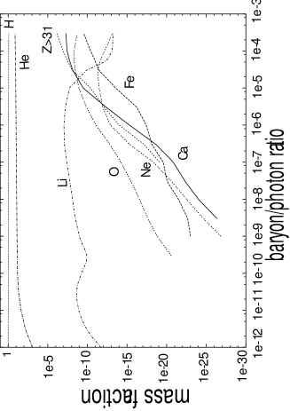
Figure 1: $\eta$ dependence of the mass fraction of each element. These of H and He are almost constant. Contrastingly, heavy elements are produced in greater abundance as $\eta$ increases, but eventually they begin to be consumed to produce even heavier elements.

The abundances of H and He remain almost constant over a wide range of values of $\eta$. C and O increase as $\eta$ increases, but eventually they reach maximum values and then decrease. Beyond that point, heavier elements, such as Ca and Fe, begin to dominate. Two typical examples of the time evolution of the abundance of each element are plotted in Figs. $2$ and $3$.

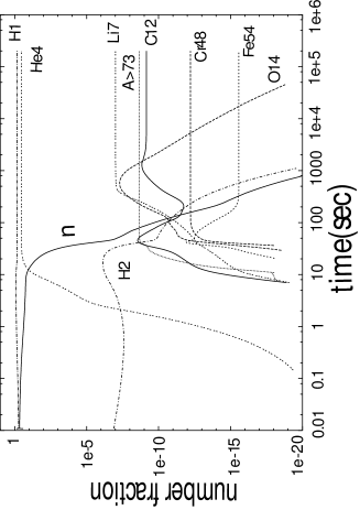
Figure 2: Time evolution with $\eta=10^{-5}$

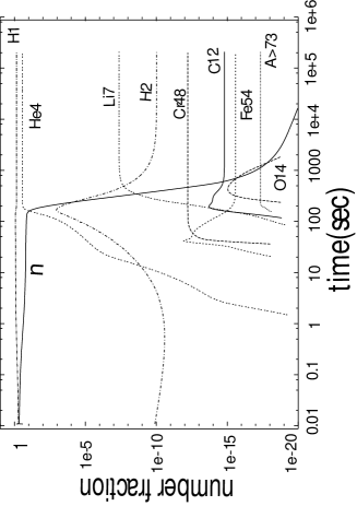
Figure 3: Time evolution of nuclei abundances with $\eta=10^{-8}$

In the early stages, there is an abundance of light elements. Then as reactions proceed the light elements are consumed, and heavy elements begin to be produced. Production of heavy elements at $\eta=10^{-5}$ is much larger than at $\eta=10^{-8}$. In particular, nuclei with mass numbers greater than 73 begin to dominate at $\eta=10^{-5}$.

In Fig. $4$ the ratio of the BBN number fraction with respect to the present solar system number fraction is presented. We find two peaks in the graph, one corresponding to calcium at Z=20, one corresponding to Germanium at Z=32. We believe that the peak value at Z=32 should not regarded as the Ge fraction but, rather, as the sum of the abundances of all elements with atomic number greater than 32, because our network includes only those nuclei with Z$\leq$32, and thus the reaction cannot proceed beyond Germanium, and the nuclei accumulate there. By contrast, the peak at Z=20 should be considered as representing a peak of calculation. To understand why Ca is produced to much a great degree, it is necessary to know which of the Ca isotopes is produced in greatest abundance. These data are presented in Table 4.

isotopes	abundances
Ca40	$5.33\times 10^{-8}$
Ca41	$1.8\times 10^{-9}$
Ca42	$1.93\times 10^{-9}$
Ca43	$1.21\times 10^{-12}$
Ca44	$1.89\times 10^{-17}$

Table 4: The abundances of Ca isotopes. This shows that Ca 40, which is the double magic number nucleus, is dominantly produced.

The table shows that the dominant output is for Ca 40, which has 20 protons and 20 neutrons. It is to be noted that 20 is a magic number, and Ca 40 is a double magic number nucleus which is known to be very stable. Surprisingly, no peak can be found at Z=26 (Fe). On the contrary, there is a decrease there. There are two reasons for this. The first is that because of the p-process, the production of Fe is inhibited. The second is that the solar abundance of Fe is large. At $\eta=3\times 10^{-4}$, [Fe/H]$=-6.70$ is still too small, but [Ca/H]$=-2.17$ is large enough to be inconsistent with the observations of extremely metal poor stars. For example, [Ca/H]$=-5.37$ for He0107-5240 [22]. In order for the Ca abundance produced at BBN to be below this value, $\eta$ of a high baryon density bubble, if surrounding this metal poor star, should be smaller than $10^{-5}$. However, there is such a great degree of freedom in our model that we cannot strongly restrict it with data from only a single observation. We can only say that if such a model is realized, $\eta$ of the bubble around this metal poor star must be under $10^{-5}$. On the other hand, it may be the case that the observed early metal poor stars are well outside of the baryon rich regions. For confirmation of the model, we need to carry out calculations with larger values of $\eta$, because for $\eta\leq 3\times 10^{-4}$, the abundances of heavy elements are still small in comparison with those observed in IGM, around QSO, and in most of the metal poor stars. Observations of objects in the early universe with anomalously high metal abundances are also desirable. To impose some restrictions on the mass of the Affleck-Dine field, its coupling strength, etc., we need additional observational data. Extending our calculations to larger values of $\eta$ in order to obtain predictions for the abundances of heavier elements, it may be possible to distinguish usual stars from our bubble-made stars, which is necessary to improve the restriction. With such progress, in the future, we may be able to reach a more definite conclusion.

There is another interesting possibility. To this point, we have considered the case in which baryons in the bubbles do not diffuse. However, if the bubbles are smaller than the quark diffusion distance, which can be evaluated [11] in comoving coordinates as $\sim$ $(tl_{free})^{1/2}$, where $l_{free}$ is the quark mean free path, $l_{free}\sim(\sigma N)^{-1}\sim T^{-1}$, they do diffuse. This could affect the angular spectrum of CMBR. Most IBBN studies carried out to this time treat only small values of $\eta$, specifically, $\eta\sim 10^{-10}$. However, with our approach, we are able to investigate a novel relation between IBBN and CMBR. Our study also suggests some possibilities for the origin of p-nuclei in the solar system. To investigate this, we need to calculate the BBN abundances with a reaction network that includes heavier nuclei. There is also the possibility that the baryon rich bubbles, though not forming primordial black holes, might end up as stellar-type or planetary-type objects. In this case (which is under investigation), the observational consequences could be quite different.

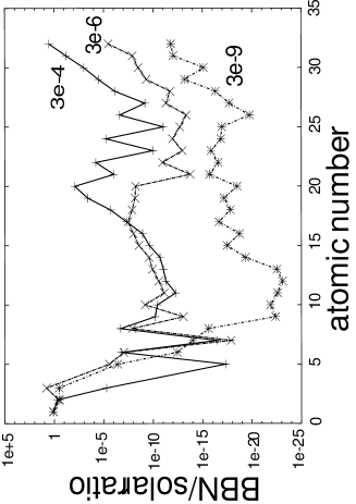
Figure 4: The ratio of BBN to the solar mass fraction for a range of elements. There is a prominent peak corresponding to Ca. We compare this Ca abundance with observation results to obtain an upper bound on $\eta$.

4 Acknowledgments

S.M. thanks Kazuhiro Yahata, Tomoya Takiwaki, Yasuko Hisamatsu and Kumiko Kihara for helping me in computer and Kazuhiro Yahata, Kohji Yoshikawa and Atsunori Yonehara for useful discussions. This research was supported in part by Grants-in-Aid for Scientific Research provided by the Ministry of Education, Science and Culture of Japan through Research Grant No.S 14102004, No.14079202 and No.16740134.

References

- [1] C.L. Bennet, et al., Astrophys. J. Suppl. 148, 1, (2003).
- [2] A.J. Barth, P. Martini, C.H. Nelson, and L.C. Ho, Astrophys. J. 594,L95 (2003)[astro-ph/0308005].
- [3] M. Dietrich, I. Appenzeller, M. Vestergaard, and S.J. Wagner, Astrophys. J. 564, 581 (2002).
- [4] A. Boksenberg, W.L.W. Sargent, and M. Rauch, [astro-ph/0307557].
- [5] C. Warner, F. Hamann, and M. Dietrich, Astrophys. J. 596, 72 (2003)[astro-ph/0307247].
- [6] R. Pello, et al., Astron. & Astrophys. 416, L35 (2004)[astro-ph/0403025].
- [7] C. Pichon,et al., Astrophys. J. 597, L97 (2003)[astro-ph/0309646].
- [8] J. G. Cohen, et al., [astro-ph/0405286]
- [9] Z. Haiman, and A. Loeb, Astrophys. J. 552, 459H (2001).
- [10] M. Tegmark, et al., Astrophys. J. 474, 1 (1997).
- [11] A. Dolgov, and J. Silk, Phys. Rev. D47, 4244 (1993).
- [12] B.D. Fields and K.A. Olive, Astrophys. J. 506, 177 (1998); S. G. Ryan, T. C. Beers, K. A. Olive, B. D. Fields, and J. E. Norris, Astrophys. J. .Letters 530, L57 (2000); P. Bonifacio, et al., Astron. & Astrophys. 390, 91 (2002); D. Kirkman, D. Tytler, N. Suzuki, J. M. O’Meara, and D. Lubin, Astrophys. J. .Suppl. 149, 1 (2003) [arXiv:astro-ph/0302006]. Y.I. Izotov and T.X. Thuan, Astrophys. J. 602, 200 (2004). and papers cited therein.
- [13] C.L. Bennett, et al., Astrophys. J. . Suppl. 148, 1 (2003)[astro-ph/0302215]; D.N. Spergel, et al., Astrophys. J. . Suppl. 148, 175 (2003)[astro-ph/0302209].
- [14] I. Affleck, and M. Dine, Nucl. Phys. B249, 361 (1985).
- [15] S. Coleman, E. Weinberg, Phys. Rev. D7, 1888 (1973).
- [16] R.H.Cyburt, B.D. Fields, and K.A. Olive, Phys. Lett. B567, 227 (2003)[astro-ph/0302431]; A.Coc, et al., [astro-ph/0401008]; R.H.Cyburt, [astro-ph/0401091].
- [17] For reviews see, S. Sarkar, Rept. Prog. Phys. 59, 1493 (1996)[hep-ph/9602260]; D. Tytler, J.M. O’Meara, N. Suzuki, and D. Lubin, [astro-ph/0001318]; K.A. Olive, G. Steigman, and T.P. Walker, Phys. Rept. 333, 389 (2000)[astro-ph/9905320]; and references in these reviews.
- [18] J.H. Applegate, C.J. Hogan, and R.J. Scherrer, Phys. Rev. D35, 1151 (1987); C. Alcock, G.M. Fuller, and G.J. Mathews, Astrophys. J. 320, 439 (1987); R.M. Malaney and W.A. Fowler, Astrophys. J 333, 14 (1988); H. Kurki-Suonio, R. A. Matzner, J. M. Centrella, T. Rothman, and J. R. Wilson, Phys. Rev. D38, 1091 (1988); N. Terasawa and K. Sato, Phys. Rev. D39, 2893 (1989); G. J. Mathews, B. S. Meyer, C. R. Alcock, and G. M. Fuller, Astrophys. J. 358, 36 (1990); K. Jedamzik, G. M. Fuller, G. J. Mathews, and T. Kajino, Astrophys. J. 422, 423 (1994); K. Jedamzik, G. M. Fuller, and G. J. Mathews, Astrophys. J. 423 50 (1994); G. J. Mathews, T. Kajino, and M. Orito, Astrophys. J. 456, 98 (1996); In-Saeng Suh and G. J. Mathews, Phys. Rev. D58, 123002 (1998); K. Kainulainen, H. Kurki-Suonio, and E. Sihvola, Phys. Rev. D59, 083505 (1999); K. Jedamzik, and J.B. Rehm, Phys. Rev. D64, 023510 (2001)[astro-ph/0101292].
- [19] S. Nagataki, M. Hashimoto, and S. Yamada, Publ. Astron. Soc. Jap. 50, 67 (1998)[astro-ph/9807014].
- [20] S. Nagataki, M. Hashimoto, K. Sato, S. Yamada, and Y.S. Mochizuki, Astrophys. J. 492, L45 (1998)[astro-ph/9807015].
- [21] N. Terasawa, and K. Sato, Astrophys. J. 294, 9 (1985).
- [22] N. Christlieb, et al., Astrophys. J. 603, 708 (2004)[astro-ph/0311173].