Dark matter and dark energy production in quantum model of the universe

Abstract

The matter/energy structure of the homogeneous, isotropic, and spatially closed universe is studied. The quantum model under consideration predicts an existence of two types of collective quantum states in the universe. The states of one type characterize a gravitational field, the others describe a matter (uniform scalar) field. In the first stage of the evolution of the universe a primordial scalar field evolves slowly into its vacuum-like state. From the point of view of semiclassical description the early universe is filled with primordial radiation and is charge symmetric in this stage. In the second stage the scalar field oscillates about an equilibrium due to the quantum fluctuations. The universe is being filled with matter in the form of elementary quantum excitations of the vibrations of the scalar field. The separate quantum excitations are characterized by non-zero values of their energies (masses). Under the action of gravitational forces mainly these excitations decay into ordinary particles (baryons and leptons) and dark matter. The elementary quantum excitations of the vibrations of the scalar field which have not decayed up to now form dark energy. The numerical estimations lead to realistic values of both the matter density $\Omega_{M}\simeq 0.29$ (with the contributions from dark matter, $\Omega_{DM}\simeq 0.25$, and optically bright baryons, $\Omega_{stars}\simeq 0.0025$) and the dark energy density $\Omega_{X}\simeq 0.71$ if one takes that the mean energy $\sim 10$ GeV is released in decay of dark energy quantum and fixes baryonic component $\Omega_{B}=0.04$ according to observational data. The energy (mass) of dark energy quantum is equal to $\sim 17$ GeV and the energy $\gtrsim 2\times 10^{10}$ GeV is needed in order to detect it. Dark matter particle has the mass $\sim 6$ GeV. The Jeans mass for dark matter which is considered as a gas of such massive particles is equal to $M_{J}\sim 10^{5}M_{\odot}$.

1 Introduction

Observations indicate that overwhelming majority (about 96%) of matter/energy in the universe is in unknown form (see e.g. Refs. [1, 2] for reviews). The observed mass of stars gives the value $\Omega_{stars}\simeq 0.005$ [3] or even smaller $\Omega_{stars}\simeq 0.003^{+0.001}_{-0.002}$ [4] for the density of visible (optically bright) baryons. Observations of the cosmic microwave background radiation (CMB) and abundances of the light elements in the universe suggest that the total density of baryons is equal to $\Omega_{B}\simeq 0.04$ [1, 2, 5]. This value is one order greater than $\Omega_{stars}$. It means that most of baryonic matter today is not contained in stars and is invisible (dark).

The CMB anisotropy measurements allow to determine the total energy density $\Omega_{tot}$ and the matter component $\Omega_{M}$. The recent data give the strong evidence that the present-day universe is spatially flat (or very close to it) with $\Omega_{tot}\simeq 1$ [6] and the mean matter density equals $\Omega_{M}\simeq 0.3$ [1]. The independent information about $\Omega_{M}$ extracted from the high redshift supernovae Ia data on the assumption that $\Omega_{tot}=1$ gives the close values: $\Omega_{M}=0.28\pm 0.05$ [7] or $\Omega_{M}=0.29^{+0.05}_{-0.03}$ [8]. The discrepancies between $\Omega_{M}$ and $\Omega_{B}$ on the one hand and $\Omega_{tot}$ and $\Omega_{M}$ on the other hand are signs that there must exist non-baryonic dark matter with the density $\Omega_{DM}=\Omega_{M}-\Omega_{B}\sim 0.3$ and some mysterious cosmic substance (so-called dark energy [9]) with the density $\Omega_{X}=\Omega_{tot}-\Omega_{M}\sim 0.7$. The origin and composition of both dark matter and dark energy are unknown. Dark matter manifests itself in the universe through the gravitational interaction. Its presence allows to explain rotation curves for galaxies and large-scale structure of the universe in the models with standard assumption of adiabatic density perturbations [1, 2, 10]. Candidates for dark matter and dark energy are discussed e.g. in reviews [1, 2, 10, 11]. As regards dark energy it is worth mentioning that its expected properties are unusual. It is unobservable (in no way could it be detected in galaxies) and spatially homogeneous.

Thus the present data of modern cosmology pose the principle question about the nature of the mass-energy constituents of the universe and their percentage in the total energy density. Efforts in this direction were focused on a choice of candidates for dark matter and dark energy between known (real or hypothetical) particles and fields. It is obvious that reasonable cosmological theory must first of all answer the question why the densities $\Omega_{M}$ and $\Omega_{X}$ in the present era are comparable between themselves (so-called coincidence problem) and explain the observed ratio $\Omega_{B}/\Omega_{stars}\sim O(10)$.

In the present paper the problem of dark matter and dark energy is studied in the context of the quantum model of the universe proposed in Refs. [12, 13]. The first attempts to give an answer to the question about the nature of dark matter and dark energy on the basis of quantum approach to cosmological problems were made in Refs. [14, 15].

In Sec. 2 the basic equations of the quantum model of the homogeneous, isotropic and spatially closed universe are given. It is supposed that the universe is filled with primordial matter in the form of the uniform scalar field. Time is introduced as an embedding variable which describes a motion of some source. From the point of view of semiclassical approach this source has a form of radiation. The evolution of the universe can be conventionally divided into two stages. At the first stage (Sec. 3) the scalar field determines the vacuum energy density which slowly evolves into the state with minimal density (vacuum-like state). Radiation is present as a primordial source and universe is charge symmetric. In Sec. 4 the second stage of the evolution of the universe in considered. At this stage the scalar field oscillates about the equilibrium vacuum-like state and the universe is being filled with matter in the form of elementary quantum excitations of the vibrations of the scalar field. These excitations have the non-zero energies (masses). The wavefunction is an amplitude of the probability wave of the universe to be in the state with given values of two quantum numbers. One quantum number characterizes the gravitational field, while another relates to the scalar field. In Sec. 5 the simple model of creation of matter in the ordinary forms as a result of decay of elementary quantum excitations of the vibrations of the scalar field under the action of gravitational forces is proposed. The numerical estimations of the percentage of dark matter and dark energy in the present-day universe are given. A comparison of theoretical calculations with integrated data from WMAP, other CMB experiments, HST key project and supernovae observations [16] is made. In Sec. 6 some conclusions are drawn.

2 Basic equations of the model

Let us consider the quantum model of the homogeneous, isotropic and spatially closed universe filled with primordial matter in the form of the uniform scalar field $\phi$ with some potential energy density $V(\phi)$. The time-dependent equation which describes such a universe has a form [12, 13] (here and below we use dimensionless variables where the length is measured in units of $l_{P}=\sqrt{2G/(3\pi)}$ and the energy density in $\rho_{P}=3/(8\pi Gl_{P}^{2})$)

$$i\,\partial_{\mathcal{T}}\Psi=\hat{\mathcal{H}}\Psi,$$ (1)

where

$$\hat{\mathcal{H}}=\frac{1}{2}\left(\partial_{a}^{2}-\frac{2}{a^{2}}\,\partial_{\phi}^{2}-a^{2}+a^{4}V(\phi)\right)$$ (2)

is a Hamiltonian-like operator. The wavefunction $\Psi$ depends on the cosmological scale factor $a$, scalar field $\phi$, and time coordinate $\mathcal{T}$. In derivation of Eq. (1) time $\mathcal{T}$ is introduced as an additional (embedding) variable which describes a motion of a source in a form of relativistic matter of an arbitrary nature from the point of view of semiclassical approach. It is related to the synchronous proper time $t$ by the differential equation: $dt=a\,d\mathcal{T}$ [12]. Eq. (1) allows a particular solution with separable variables

$$\Psi=\mbox{e}^{\frac{i}{2}E\mathcal{T}}\psi_{E},$$ (3)

where the function $\psi_{E}$ is given in $(a,\phi)$-space of two variables and satisfies the time-independent equation

$$\left(-\,\partial_{a}^{2}+a^{2}-a^{4}\hat{\rho}_{\phi}-E\right)\psi_{E}=0.$$ (4)

Here the operator

$$\hat{\rho}_{\phi}=-\,\frac{2}{a^{6}}\,\partial_{\phi}^{2}+V(\phi)$$ (5)

corresponds to the energy density of the scalar field in classical theory (cf. e.g. Ref. [11]). The eigenvalue $E$ determines the components of the energy-momentum tensor $\widetilde{T}^{0}_{0}=E/a^{4}$ and $\widetilde{T}^{\mu}_{\nu}=-\,E/(3\,a^{4})\,\delta^{\mu}_{\nu}$, where $\mu,\nu=1,2,3$. We shall consider the case $E>0$ and call a source determined by the energy-momentum tensor $\widetilde{T}^{\mu}_{\nu}$ a radiation.

In order to find the function $\psi_{E}$ at given $V(\phi)$ Eq. (4) must be supplemented with the boundary condition. According to Eq. (4) the universe can be both in quasistationary and continuum states [12]. Quasistationary states are the most interesting since the universe in such states can be described by the set of standard cosmological parameters [13]. These states are characterized by some complex parameter $E=E_{n}+i\,\Gamma_{n}$, where $E_{n}>0$ is a position, $\Gamma_{n}>0$ is a width of the $n$-th level, $n=0,1,2,\ldots$. The wavefunction $\psi_{E}$ of the quasistationary state as a function of $a$ has a sharp peak and it is concentrated mainly in the region limited by the barrier $U=a^{2}-a^{4}V(\phi)$ (see Eq. (4)). It can be normalized [17] and used in calculations of expectation values of operators corresponding to observed parameters within the lifetime of the universe, when the quasistationary states can be considered as stationary ones with $E=E_{n}$ (cf. e.g. Ref. [18]). Such an approximation does not take into account exponentially small probability of tunneling through the barrier $U$. Below we shall not go beyond this approximation.

3 First stage of evolution

It is convenient to divide the evolution of the universe conventionally into two stages. Let us assume that at the first stage the scalar field $\phi$ evolves slowly (in comparison with a large increase of the average value of the scale factor $\langle a\rangle$ in the state $\psi_{E}$ normalized as described above) from some initial state $\phi_{start}$, where $V(\phi_{start})\sim\rho_{P}$, into a vacuum-like state with $V(\phi_{vac})=0$. During this era from the point of view of semiclassical description the early universe is filled with primordial radiation and is charge symmetric. The scalar field $\phi$ forms a vacuum state with the non-zero energy density, $V(\phi(t))\neq 0$, which effectively decreases with time $t$. At this stage the kinetic term of the operator of the energy density of the scalar field (5) can be neglected (adiabatic approximation), and it is convenient to represent the wavefunction of the universe in the $n$-th state, $\psi_{E}=|E_{n}\rangle$, in the form of expansion in terms of a complete set of functions $\langle a|n\rangle$ which satisfy the equation

$$\left(-\,\partial_{a}^{2}+a^{2}-\epsilon_{n}^{0}\right)|n\rangle=0,$$ (6)

where $\epsilon_{n}^{0}=4n+3$. Then we have

$$|E_{n}\rangle=\sum_{q}|q\rangle\langle q|E_{n}\rangle.$$ (7)

Taking into account that quasistationary states are realized in the universe only in the case when $V\ll 1$ [12, 13] and using the perturbation theory we obtain

$$\langle q|E_{n}\rangle=\delta_{nq}-\frac{V}{4}\left[\frac{1}{8}\sqrt{N(N-1)(N-2)(N-3)}\right.\delta_{n-2,q}$$ (8)

$$+\sqrt{N(N-1)}\left(N-\frac{1}{2}\right)\delta_{n-1,q}-\sqrt{(N+1)(N+2)}\left(N+\frac{3}{2}\right)\delta_{n+1,q}$$

$$-\left.\frac{1}{8}\sqrt{(N+1)(N+2)(N+3)(N+4)}\,\delta_{n+2,q}\right]-O(V^{2}),$$

where $N=2n+1$. The eigenvalue $E$ in this approximation is the following

$$E_{n}=2N+1-\frac{3}{4}\,V\,[2N(N+1)+1]-O(V^{2}).$$ (9)

It depends on $\phi$ parametrically. The wavefunction $\langle a|n\rangle$ describes the geometrical properties of the universe as a whole. Since in classical theory the gravitational field is considered as a variation of space-time metric, then this wavefunction will characterize the quantum properties of the gravitational field. The states $\langle a|n\rangle$ can be formally interpreted as those which emerge as a result of motion of some imaginary particle with the Planck mass $m_{P}=l_{P}^{-1}$ and zero orbital angular momentum in imaginary field with the potential energy $U(R)=\frac{1}{2}\,k_{P}R^{2}$, where $R=l_{P}a$ is a “radius” of the curved universe, while $k_{P}=m_{P}^{3}$ can be called a “stiffness coefficient of gravitational field (or space)”. Its numerical value is $k_{P}=4.79\times 10^{85}$ GeV $\mbox{cm}^{-2}$. This motion causes the equidistant spectrum of energy $\mathcal{E}_{n}=m_{P}\left(N+\frac{1}{2}\right)$, where $m_{P}$ is the energy (mass) of the elementary quantum excitation of the vibrations of the oscillator (6).

Introducing the operators

$$A^{{\dagger}}=\frac{1}{\sqrt{2}}\,(a-\partial_{a}),\quad A=\frac{1}{\sqrt{2}}\,(a+\partial_{a}),$$ (10)

the state $|n\rangle$ can be represented in the form

$$|n\rangle=\frac{1}{\sqrt{N!}}\,(A^{{\dagger}})^{N}\,|vac\rangle,\quad A\,|vac\rangle=0,\quad|vac\rangle=\left(\frac{4}{\pi}\right)^{1/4}\exp\left\{-\frac{a^{2}}{2}\right\}.$$ (11)

The operators $A^{{\dagger}}$ and $A$ satisfy the ordinary canonical commutation relations, $[A,A^{{\dagger}}]=1,\ [A,A]=[A^{{\dagger}},A^{{\dagger}}]=0$, and one can interpret them as the operators for the creation and annihilation of the elementary quantum excitation with the energy $m_{P}$. The integer $N$ gives the number of these excitations in the $n$-th state of the universe. The vacuum state $|vac\rangle$ describes the universe without such excitations. From Eqs. (7) and (8) it follows that the universe can be characterized by quantum number $n$. In such a description the gravitational field is considered as a system of the elementary quantum excitations of the vibrations of the oscillator (6).

The interaction between the gravitational field and non-zero vacuum of the field $\phi$ results in the fact that the wavefunction (7) is a superposition of the states with different $n$.

When the potential energy density $V(\phi)$ decreases to the value $V\ll 0.1$ the number of available states of the universe increases up to $n\gg 1$. By the moment when the scalar field will roll in the location where $V(\phi_{vac})=0$ the universe can be found in the state with $n\gg 1$. This can occur because the emergence of new quantum levels and the (exponential) decrease in widthes of old ones result in the appearance of the competition between the tunneling through the barrier $U$ and allowed transitions between the states $n\rightarrow n\pm 1,\ n\pm 2$ (see Eq. (8)). A comparison between these processes demonstrates [12, 13] that the transition $n\rightarrow n+1$ is more probable than any other allowed transitions or decays. The vacuum energy in the early universe originally stored by the field $\phi$ with the potential energy density $V(\phi_{start})\sim\rho_{P}$ is a source of transitions with increase in number $n$.

4 Creation of matter/energy

According to accepted model the scalar field $\phi$ descends to the state with zero energy density, $V(\phi_{vac})=0$. At that instant the first stage comes to an end and the universe enters the second stage of its evolution. The main feature of the new era is a creation of matter/energy which can turn into the ordinary forms. In the state with $V(\phi_{vac})=0$ the field $\phi$ oscillates about the equilibrium vacuum-like state due to quantum fluctuations. These oscillations can be quantized.

In general case it is convenient to represent the wavefunction $\psi_{E}$ of Eq. (4) in the form of a superposition of the states of adiabatic approximation. In the case of the states with $n\gg 1$ which we shall study the task is simplified. Since the expansion coefficients of the adiabatic wavefunction (7) behave as

$$\langle q|E_{n}\rangle\rightarrow\delta_{nq}\quad\mbox{for}\quad n\rightarrow\infty$$ (12)

up to the terms $\sim O(V^{2})$, then the wavefunction in the states with $n\gg 1$ in adiabatic approximation coincides with the function $\langle a|n\rangle$ with above accuracy. And the desired representation of the wavefunction $\psi_{E}$ has a form $\psi_{E}=\sum_{n}|n\rangle\,f_{n}$. Multiplying Eq. (4) by $a^{2}$ on the left and using this expansion, one obtains the set of equations for the coefficients $f_{n}$ as functions of $\phi$. In the limit $n\gg 1$ such a set is reduced to one equation. This equation coincides with the equation which follows from Eq. (4), if one uses the expansion of the wavefunction $\psi_{E}$ in terms of a complete set of exact functions of adiabatic approximation and then passes to limit of very large numbers $n$ in a final set of equations for the coefficients of expansion [12].

We are interested in the states of the field $\phi$ near its vacuum value $\phi_{vac}$. Therefore it is convenient to pass in equation for $f_{n}$ from the variable $\phi$ to $x\sim(\phi-\phi_{vac})$ which characterizes a deviation of $\phi$ from equilibrium value $\phi_{vac}$. Such an equation has a form

$$\left[\partial_{x}^{2}+z-V(x)\right]f_{n}(x)=0,$$ (13)

where $x=\sqrt{m/2}\,(2N)^{3/4}\,(\phi-\phi_{vac})$, $z=(\sqrt{2N}/m)\left(1-E/(2N)\right)$, and $V(x)=(2N)^{3/2}\,V(\phi)/m$, $m$ is some dimensionless parameter. Since the average value of the scale factor in the state of the universe with $n\gg 1$ is equal to $\langle a\rangle=\sqrt{N/2}$ [12, 13], then $V(x)$ is the potential energy of the scalar field contained in the universe with the volume $\sim\langle a\rangle^{3}$. The value $x^{2}$ characterizes the deviation squared of the field $\phi$ in the volume $\sim\langle a\rangle^{3}$. Therefore Eq. (13) describes the stationary states which characterize the scalar field $\phi$ in the universe as a whole.

Choosing the parameter $m^{2}=\left[\partial_{\phi}^{2}V(\phi)\right]_{\phi_{vac}}$ and expanding $V(\phi)$ in the powers of $x$ we obtain

$$V(x)=x^{2}+\alpha\,x^{3}+\beta\,x^{4}+\ldots,$$ (14)

where

$$\alpha=\frac{\sqrt{2}}{3}\,\frac{\lambda}{m^{5/2}}\,\frac{1}{(2N)^{3/4}},\quad\beta=\frac{1}{6}\,\frac{\nu}{m^{3}}\,\frac{1}{(2N)^{3/2}},$$ (15)

and $\lambda=\left[\partial_{\phi}^{3}V(\phi)\right]_{\phi_{vac}}$, $\nu=\left[\partial_{\phi}^{4}V(\phi)\right]_{\phi_{vac}}$. The potential energy density $V(\phi)$ near the point $\phi_{vac}$ will be considered to be smooth sufficiently so that $m^{2}>\lambda>\nu$.

Since $N\sim n\gg 1$, then $|\alpha|\ll 1$, $|\beta|\ll 1$, and Eq. (13) can be solved using the perturbation theory for stationary problems with a discrete spectrum. We take for the state of the unperturbed problem the state of the harmonic oscillator with the equation of motion (13), where $V(x)=x^{2}$. In the occupation number representation one can write for the unperturbed states

$$f_{ns}^{0}=\frac{1}{\sqrt{s!}}\,(B_{n}^{{\dagger}})^{s}f_{n0}^{0},\quad B_{n}\,f_{n0}^{0}=0,\quad f_{n0}^{0}(x)=\left(\frac{1}{\pi}\right)^{1/4}\exp\left\{-\frac{x^{2}}{2}\right\}$$ (16)

with $z^{0}=2s+1$, where $s=0,1,2\ldots$, and it is denoted

$$B_{n}^{{\dagger}}=\frac{1}{\sqrt{2}}\,(x-\partial_{x}),\qquad B_{n}=\frac{1}{\sqrt{2}}\,(x+\partial_{x}).$$ (17)

Solving Eq. (13) with the potential (14) we find

$$z=2s+1+\Delta z,$$ (18)

where

$$\Delta z = \frac{3}{2}\beta\left(s^{2}+s+\frac{1}{2}\right)-\frac{15}{8}\alpha^{2}\left(s^{2}+s+\frac{11}{30}\right)$$ (19)

$$- \frac{\beta^{2}}{16}\left(34s^{3}+51s^{2}+59s+21\right).$$

The spectrum of the energy states of the field $\phi$ has a form

$$M_{s}=m\left(s+\frac{1}{2}\right)+\Delta M,$$ (20)

where $\Delta M=m\Delta z/2$. The operators $B_{n}^{{\dagger}}$ and $B_{n}$ satisfy the ordinary canonical commutation relations, $[B_{n},B_{n}^{{\dagger}}]=1,\ [B_{n},B_{n}]=[B_{n}^{{\dagger}},B_{n}^{{\dagger}}]=0$, and can be interpreted as the creation ($B_{n}^{{\dagger}}$) and annihilation ($B_{n}$) operators which increase and decrease the number of elementary quantum excitations of the vibrations of the scalar field by unity in the universe in the $n$-th state, respectively. Therefore it is natural to interpret the value $M=m(s+1/2)$ as a quantity of matter/energy being the sum of elementary quantum excitations of the vibrations of the field $\phi$ with the energy (mass) $m$, while $s$ counts the number of these excitations. It can be considered as additional quantum number. The summand $\Delta M$ in Eq. (20) takes into account a self-action of the elementary quantum excitations of the vibrations of the field $\phi$.

Using Eq. (18) and the relation between $z$ and $E$ we find the condition of quantization

$$E=2N-\sqrt{2N}M_{s}.$$ (21)

This condition can be rewritten in terms of classical cosmology in the form of the relation between the parameters of the universe

$$\langle a\rangle=M_{s}+\frac{E}{4\langle a\rangle},$$ (22)

where $\langle a\rangle$ is the scale factor, $M_{s}$ is the energy of matter (in the form of a system of elementary quantum excitations of the vibrations of the scalar field), while $E/(4\langle a\rangle)$ is the energy of radiation.

Let us estimate $\Delta M/M$. Substituting Eq. (15) into (19), leaving the main terms only, and taking in accordance with Eq. (22) that $\langle a\rangle\sim ms$ we obtain

$$\frac{\Delta M}{M}\sim\left[0.02\,\frac{\nu}{m^{2}}-0.03\,\left(\frac{\lambda}{m^{2}}\right)^{2}\right]\frac{1}{(m^{2}s)^{2}}-4.6\times 10^{-4}\left(\frac{\nu}{m^{2}}\right)^{2}\frac{1}{(m^{2}s)^{4}}.$$ (23)

From here it follows that

$$\frac{\Delta M}{M}\ll 1\quad\mbox{at}\quad s>m^{-2}.$$ (24)

Let us estimate the value $s$ at which condition of smallness of $\Delta M/M$ is satisfied. In the limit of maximum possible mass $m\sim 1\,(\sim 10^{19}\,\mbox{GeV})$ we find $s>1$. Such a universe has the parameters: $M>1\,(\sim 10^{19}\,\mbox{GeV})$, $\langle a\rangle>1\,(\sim 10^{-33}\,\mbox{cm})$ and age $t>1\,(\sim 10^{-44}\,\mbox{s})$. Taking $s\sim 10^{80}$ (equivalent number of baryons in the present-day universe) we obtain the limitation on mass from below, $m>10^{-40}\,(\sim 10^{-21}\,\mbox{GeV})$. Assuming that $m\sim 10^{-18}\,(\sim 10\,\mbox{GeV})$ we find the following restriction on the number of elementary quantum excitations of the vibrations of the field $\phi$: $s>10^{36}$. The quantity of matter/energy in such a universe is $M>10^{18}\,(\sim 10^{37}\,\mbox{GeV})$, radius of curvature $\langle a\rangle>10^{18}\,(\sim 10^{-15}\,\mbox{cm})$, and age $t>10^{-26}$ s. Below (in Sec. 5) we shall consider the model of creation of ordinary matter which leads to $m\gtrsim 10$ GeV.

At the end of this section let us calculate the mean energy density in the universe in the states with large quantum numbers. From Eq. (4) it follows that the operator

$$\hat{\rho}_{tot}=\hat{\rho}_{\phi}+\frac{E}{a^{4}}$$ (25)

corresponds to the total energy density in classical theory. Then the average value $\langle\hat{\rho}_{tot}\rangle$ in the state of the universe with $n\gg 1$, $s\gg 1$ is

$$\langle\hat{\rho}_{tot}\rangle=\gamma\frac{M}{\langle a\rangle^{3}}+\frac{E}{\langle a\rangle^{4}},$$ (26)

where $\gamma=193/12$ and it is assumed that the average value $\langle a\rangle$ determines the scale factor of the universe in semiclassical description (details can be found in Refs. [12, 13, 19]). In this approximation the universe is described by the Einstein-Friedmann equations in terms of average values which follow from Eq. (4) and from Heisenberg-type equation. The latter determines a change in time of the average values of the physical quantities [19]. In the matter dominated universe $M\gg E/(4\langle a\rangle)$ and the mean energy density (26) leads to the dimensionless density $\Omega_{tot}\equiv\langle\hat{\rho}_{tot}\rangle/H^{2}=1.066$, where $\langle\hat{\rho}_{tot}\rangle$ is measured in units of $\rho_{P}$ and the Hubble constant $H$ in inverse Planck time $t_{P}^{-1}=l_{P}^{-1}$. It means that the universe in highly excited states is very close to being spatially flat. It agrees with existing astrophysical data for the present-day universe (see Sec. 1). Moreover a very slight systematical excess of $\Omega_{tot}$ over unity is observed [16].

5 Dark matter and baryonic matter production

The elementary quantum excitations of the vibrations of the field $\phi$ are subject to action of gravity. Due to this fact they can decay into the ordinary particles (e.g. baryons and leptons) that have to be present in the universe in small amount because of the weakness of the gravitational interaction.

As it is mentioned in Sec. 1 the total energy density can be represented as a sum of three terms

$$\Omega_{tot}=\Omega_{B}+\Omega_{DM}+\Omega_{X}.$$ (27)

Therefore in simple (naive) model it is natural to assume that the elementary quantum excitation (let us denote it by $\phi$ as well) of the vibrations of the scalar field decays according to a scheme

$$\phi\longrightarrow\phi^{\prime}+\nu\,+\!\!\!\! n$$ (28)

$$\rvert$$

$$\!\!\!\!\!\!\longrightarrow p+e^{-}+\overline{\nu}$$

with stable particles in the final state. Here $\phi^{\prime}$ is the quantum of the residual excitations of the vibrations of the scalar field. A system of such quanta reveals itself in the universe in the form of non-baryonic dark matter. Neutrino $\nu$ takes away the spin, and the dark matter particle is a boson. At the first stage of decay chain (28) the baryon number is not conserved but the spin and the energy are conserved. A system of the elementary quantum excitations of the vibrations of the scalar field can be interpreted as dark energy (see below). Such elementary quantum excitations we shall call dark energy quanta for briefness. Assuming that dark energy quanta decay independently, as well as neutrons $n$, one can write a set of equations for decay chain (28) as follows

$$\frac{ds(t)}{dt}\!\!\! = \!\!\!-\Gamma_{\phi}(t)\,s(t),\quad\frac{ds_{n}(t)}{dt}=-\Gamma_{n}(t)\,s_{n}(t)+\Gamma_{\phi}(t)\,s(t),$$

$$\frac{ds_{p}(t)}{dt}\!\!\! = \!\!\!-\Gamma_{p}(t)\,s_{p}(t)+\Gamma_{n}(t)\,s_{n}(t),$$ (29)

where $s(t)$ is the number of dark energy quanta as a function of time $t$, $s_{n}(t)$ and $s_{p}(t)$ are the numbers of neutrons and protons at some instant of time $t$, $\Gamma_{\phi}(t)$ and $\Gamma_{n}(t)$ are the decay rates of dark energy quantum and neutron respectively, while the decay rate of proton will be supposed to be zero below, $\Gamma_{p}(t)=0$. The initial conditions have the form

$$s(t^{\prime})=s,\quad s_{n}(t^{\prime})=0,\quad s_{p}(t^{\prime})=0,$$ (30)

where $s$ is the number of dark energy quanta at some arbitrary chosen initial instant of time $t^{\prime}$. The first equation of the set (5) describes the exponential law of decrease of the number of dark energy quanta with time,

$$s(t)=s\,\mbox{e}^{-\overline{\Gamma}_{\phi}\,\Delta t},$$ (31)

where

$$\overline{\Gamma}_{\phi}=\frac{1}{\Delta t}\int_{t^{\prime}}^{t}\!dt\,\Gamma_{\phi}(t)$$ (32)

is the mean decay rate on the interval $\Delta t=t-t^{\prime}$. Substituting (31) into the second equation of the set (5) and taking into account (30) we obtain the law of production of neutrons

$$s_{n}(t)=s\int_{t^{\prime}}^{t}\!d\tau\,\Gamma_{\phi}(\tau)\,\exp\left\{-\int_{t^{\prime}}^{\tau}\!dt^{\prime\prime}\,\Gamma_{\phi}(t^{\prime\prime})-\int_{\tau}^{t}\!dt^{\prime\prime}\,\Gamma_{n}(t^{\prime\prime})\right\}.$$ (33)

The number of protons will be

$$s_{p}(t)=s\int_{t^{\prime}}^{t}\!d\tau\,\Gamma_{n}(\tau)\,\int_{t^{\prime}}^{\tau}\!d\tau^{\prime}\,\Gamma_{\phi}(\tau^{\prime})\,\exp\left\{-\int_{t^{\prime}}^{\tau^{\prime}}\!dt^{\prime\prime}\,\Gamma_{\phi}(t^{\prime\prime})-\int_{\tau^{\prime}}^{\tau}\!dt^{\prime\prime}\,\Gamma_{n}(t^{\prime\prime})\right\}.$$ (34)

The decay rates $\Gamma_{n}(t)$ and $\Gamma_{\phi}(t)$ in Eqs. (33) and (34) are unknown. Let us assume that in the decay (28) free particles are produced and the energy is released. Then we can write energy balance equation for the decay of dark energy quantum with the energy $m$

$$m=m_{\phi^{\prime}}+m_{n}+m_{\nu}+Q,$$ (35)

where $m_{\phi^{\prime}}$, $m_{n}$, and $m_{\nu}$ are the masses of dark matter particle, neutron and neutrino, respectively, and

$$Q=\sum_{i}\left(\sqrt{m_{i}^{2}+p_{i}^{2}}-m_{i}\right),\quad i=\{\phi^{\prime},n,\nu\},$$ (36)

is the energy released in the decay, $p_{i}$ is the momentum of the particle $i$. The summand $m_{\nu}$ in Eq. (35) we shall include in $m_{\phi^{\prime}}$ considering neutrinos as a constituent part of dark matter.

At high temperatures $T\sim Q$ (small ages $t$) the rate $\Gamma_{n}$ is proportional to fifth power of temperature, $\Gamma_{n}\sim T^{5}$. When the temperature decreases (during the expansion of the universe) the rate $\Gamma_{n}$ decreases as well and at low temperatures ($t\gg 1$ s) it tends to the mean decay rate of free neutron, $\overline{\Gamma}_{n}=1.12\times 10^{-3}\ \mbox{s}^{-1}$. Therefore for estimation it is enough to take as $\Gamma_{n}(t)$ its smallest value $\overline{\Gamma}_{n}$. Moreover we shall assume that the mean decay rate of dark energy quantum (32) depends very weakly on averaging interval. Then in indicated approximation from Eqs. (33) and (34) we obtain the simple expressions

$$\frac{s_{n}(t)}{s}=\frac{\overline{\Gamma}_{\phi}}{\overline{\Gamma}_{n}-\overline{\Gamma}_{\phi}}\left(\mbox{e}^{-\overline{\Gamma}_{\phi}\Delta t}-\mbox{e}^{-\overline{\Gamma}_{n}\Delta t}\right),$$ (37)

$$\frac{s_{p}(t)}{s}=1+\frac{1}{\overline{\Gamma}_{n}-\overline{\Gamma}_{\phi}}\left(\overline{\Gamma}_{\phi}\mbox{e}^{-\overline{\Gamma}_{n}\Delta t}-\overline{\Gamma}_{n}\mbox{e}^{-\overline{\Gamma}_{\phi}\Delta t}\right).$$ (38)

It is easy to make sure that the law of conservation of number of particles, $s=s(t)+s_{n}(t)+s_{p}(t)$, holds at every instant of time $t$. Since we are interested in matter/energy density in the present-day universe, then for numerical estimations we choose $\Delta t$ equal to the age of the universe, $\Delta t=14$ Gyr [11, 20]. In this case $\overline{\Gamma}_{n}\Delta t=5\times 10^{14}\gg 1$. We suppose that the decay of dark energy quantum is caused mainly by the action of gravitational forces, so that $\overline{\Gamma}_{\phi}\ll\overline{\Gamma}_{n}$. Then Eq. (38) is simplified

$$s_{p}(t)=\overline{s}=s\,\left(1-\mbox{e}^{-\overline{\Gamma}_{\phi}\Delta t}\right),$$ (39)

where $\overline{s}$ is an average number of dark energy quanta which decay during the time interval $\Delta t$. Since dark matter particles $\phi^{\prime}$ are assumed to be stable (with lifetime greater than $\Delta t$) their number is equal to $\overline{s}$ as well. The mean decay rate $\overline{\Gamma}_{\phi}$ is unknown and must be calculated on the basis of vertex modelling of complex decay (28) or extracted from astrophysical data.

According to Eq. (26) in the matter dominated universe the total energy density $\Omega_{tot}$ for sufficiently large number $s$ of dark energy quanta equals

$$\Omega_{tot}=\gamma\,\frac{ms}{\langle a\rangle^{3}H^{2}}.$$ (40)

The densities of (both optically bright and dark) baryons and dark matter are equal to

$$\Omega_{B}=\gamma\,\frac{m_{p}\,\overline{s}}{\langle a\rangle^{3}H^{2}},\quad\Omega_{DM}=\gamma\,\frac{m_{\phi^{\prime}}\,\overline{s}}{\langle a\rangle^{3}H^{2}},$$ (41)

where $m_{p}=0.938$ GeV is a proton mass. Since the density of visible baryons is equal to a ratio of total mass to volume, then in accepted units

$$\Omega_{stars}=\frac{m_{p}\,\overline{s}}{\langle a\rangle^{3}H^{2}}.$$ (42)

Then from Eqs. (41) and (42) it follows that the coefficient $\gamma$ determines a ratio between the densities

$$\frac{\Omega_{B}}{\Omega_{stars}}\simeq 16.08.$$ (43)

On the order of magnitude this value agrees with the observational data (see Sec. 1).

Taking into account Eqs. (27), (40), (41) and (42) we obtain the following expressions for the energy density components

$$\frac{\Omega_{B}}{\Omega_{tot}}=\frac{m_{p}}{m}\,\frac{\overline{s}}{s},\quad\frac{\Omega_{DM}}{\Omega_{tot}}=\left(1-\frac{Q+m_{n}}{m}\right)\,\frac{\overline{s}}{s},$$ (44)

and

$$\frac{\Omega_{M}}{\Omega_{tot}}=\left(1-\frac{Q+\Delta m}{m}\right)\,\frac{\overline{s}}{s},\quad\frac{\Omega_{X}}{\Omega_{tot}}=1-\frac{\Omega_{M}}{\Omega_{tot}},$$ (45)

where $\Delta m=m_{n}-m_{p}=1.293$ MeV. All components are expressed in terms of three unknown parameters: $\overline{\Gamma}_{\phi}$, $m$ and $Q$.

Let us introduce the dimensionless gravitational coupling constant $g=Gm^{2}$ for a particle with mass $m$. Then using Eq. (39) the baryonic component can be rewritten as

$$\frac{\Omega_{B}}{\Omega_{tot}}=\sqrt{\frac{g_{p}}{g}}\,\left(1-\mbox{e}^{-\overline{\Gamma}_{\phi}\Delta t}\right),$$ (46)

where $g_{p}=0.590\times 10^{-38}$ is the gravitational coupling constant for a proton. In order to find the possible form of $\overline{\Gamma}_{\phi}$ as a function of $g$ let us use an analogy and take as an example the rate of decay of some particle $B$ into a pair of leptons (see e.g. Ref. [21])

$$\Gamma(B\rightarrow e^{+}e^{-})=\frac{16\pi}{3}\,\alpha^{2}\,\frac{|\psi(0)|^{2}}{\mu^{2}},$$ (47)

where $\alpha$ is the dimensionless fine-structure constant, $\mu$ is the mass of a particle $B$, $\psi(0)$ is its wavefunction at the origin. The factor $|\psi(0)|^{2}$ is a particle number density and the value $L\sim|\psi(0)|^{-2/3}$ gives a linear dimension of an area from which the pair $e^{+}e^{-}$ is emitted. On the order of magnitude $L$ characterizes a size of a particle $B$. Making substitutions $\alpha\rightarrow g$, $\mu\rightarrow m$ we obtain the expression for $\overline{\Gamma}_{\phi}$

$$\overline{\Gamma}_{\phi}=8\pi^{2}g\,|\psi(0)|^{2},$$ (48)

where $\psi(0)$ is the wavefunction of the dark energy quantum at the origin.

According to Eqs. (46) and (48) for fixed $\Delta t$ the density $\Omega_{B}$ is the function of $g$. It vanishes at $g=0$ and tends to zero as $g^{-1/2}$ at $g\rightarrow\infty$. It has one maximum. Let us fix the coupling constant $g$ by maximum value of $\Omega_{B}(g)$. Then we obtain

$$\overline{\Gamma}_{\phi}\,\Delta t=1.256.$$ (49)

For $\Delta t=14$ Gyr it gives

$$\overline{\Gamma}_{\phi}=2.840\times 10^{-18}\ \mbox{s}^{-1}.$$ (50)

This rate satisfies inequality $\overline{\Gamma}_{\phi}\ll\overline{\Gamma}_{n}$, and

$$\overline{\Gamma}_{\phi}>H_{0},$$ (51)

where $H_{0}=71\ \mbox{km s}^{-1}\mbox{Mpc}^{-1}$ is the present-day value of the Hubble expansion rate [20, 22]. The latter condition means that on average at least one interaction has occurred over the lifetime of the universe.

Substituting Eq. (49) into (39) we find

$$\frac{\overline{s}}{s}=0.715,$$ (52)

i.e. about $70$% of all elementary excitations of the vibrations of the primordial scalar field had to decay during the elapsed time $\Delta t=14$ Gyr.

If one knows $\overline{\Gamma}_{\phi}$ and $\psi(0)$, then using Eq. (48) it is possible, in principle, to restore the coupling constant $g$. But the wavefunction of dark energy quantum, as well as an equation it must satisfy, is unknown. Therefore let us consider an inverse problem. Namely, using the observed value of $\Omega_{B}$ we shall restore $g$ and then obtain all masses and density components. For definiteness we choose $\Omega_{B}/\Omega_{tot}=0.04$. Then from Eq. (43) we find the density of visible baryons

$$\frac{\Omega_{stars}}{\Omega_{tot}}=0.0025.$$ (53)

For a flat universe this value is in good agreement with observations (see Sec. 1). Then using Eqs. (44) and (52) we find

$$g\simeq 320\,g_{p},\qquad m\simeq 16.8\,\mbox{GeV}.$$ (54)

The restriction on the energy $Q$ follows from the condition $m_{\phi^{\prime}}\geq 0$

$$0\ \mbox{GeV}\leq Q\leq 15.8\ \mbox{GeV}$$ (55)

with central value $\overline{Q}=7.9$ GeV. It, in turn, leads to following restrictions on the mass of dark matter particle and on the density components

$$0\ \mbox{GeV}<m_{\phi^{\prime}}<15.8\ \mbox{GeV}$$ (56)

with central value $\overline{m}_{\phi^{\prime}}=7.9$ GeV,

$$0<\frac{\Omega_{DM}}{\Omega_{tot}}<0.67$$ (57)

with central value $\overline{\Omega}_{DM}/\Omega_{tot}\simeq 0.34$,

$$0.04<\frac{\Omega_{M}}{\Omega_{tot}}<0.71$$ (58)

with central value $\overline{\Omega}_{M}/\Omega_{tot}\simeq 0.38$,

$$0.96>\frac{\Omega_{X}}{\Omega_{tot}}>0.29$$ (59)

with central value $\overline{\Omega}_{X}/\Omega_{tot}\simeq 0.62$. Here the left-hand sides of the inequalities correspond to $Q=15.8$ GeV, while the right-hand sides to $Q=0$ GeV. From inequality (59), in particular, it follows that if practically all energy of the elementary quantum excitation of the vibrations of the scalar field transforms into the energy $Q$, then $\Omega_{X}\sim\Omega_{tot}$.

The central values of the density components $\overline{\Omega}_{DM}$ and $\overline{\Omega}_{M}$ mentioned above are undoubtedly overestimated, since they take into account the upper limits for these components corresponding to unlikely value $Q=0$ GeV. In naive model (28) under consideration it make sense to speak only about the order of magnitude of the mean energy $Q$, which according to Eq. (55) is equal to $Q\simeq 10$ GeV. The following parameters correspond to such an energy

$$\frac{\Omega_{DM}}{\Omega_{tot}}\simeq 0.25,\quad\frac{\Omega_{M}}{\Omega_{tot}}\simeq 0.29,\quad\frac{\Omega_{X}}{\Omega_{tot}}\simeq 0.71,$$ (60)

and $m_{\phi^{\prime}}\simeq 5.8$ GeV. In Figs. 1 and 2 the theoretical values of densities $\Omega_{M}/\Omega_{tot}$ (58) and $\Omega_{X}/\Omega_{tot}$ (59) in comparison with observational data summarized in Ref. [16] are shown. There is a good agreement between combined observational data (Fig. 2) and the theoretical prediction (point D corresponding to the case $Q\simeq 10$ GeV).

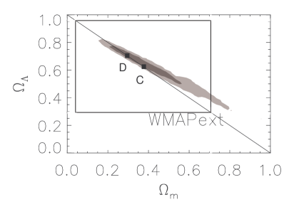
Figure 1: The plane $\Omega_{\Lambda}\equiv\Omega_{X}/\Omega_{tot}$ vs. $\Omega_{m}\equiv\Omega_{M}/\Omega_{tot}$. Constraints on the density components determined using WMAP + other CMB experiments (from Ref. [16]). The acceptable values of $\Omega_{\Lambda}$ and $\Omega_{m}$ (in accordance with inequalities (58) and (59)) lie on the diagonal of rectangle. The central value of the region is shown as a solid box C. The point D corresponds to the case $Q\simeq 10$ GeV.

Figure 2: Constraints on the density of matter $\Omega_{m}$ and dark energy $\Omega_{\Lambda}$ determined using WMAPext + HST key project data + supernova data (from Ref. [16]). The rest as in Fig. 1.

Substituting the decay rate (50) (multiplied on the Planck time $t_{P}$) and the coupling constant $g$ from Eq. (54) into Eq. (48) we obtain the following value for the dark energy quantum number density

$$|\psi(0)|^{2}\simeq\left(10^{-24}\,\mbox{cm}\right)^{-3}.$$ (61)

This estimation demonstrates that the decay of the elementary quantum excitation of the vibrations of the scalar field according to a scheme (28) occurs in an area with linear dimension $L\sim 10^{-24}$ cm corresponding to the energy $\sim 2\times 10^{10}$ GeV.

6 Conclusion

According to the model under consideration the universe in the states with large quantum numbers can be described by the superposition of quantum states of two oscillators. One oscillator describes gravitational component as a system of massive elementary quantum excitations related to the vibrations of geometry. Another oscillator describes elementary quantum excitations of the vibrations of primordial matter represented by the uniform scalar field. The latter excitations are spatially homogeneous and they form nonluminous (dark) energy. Mainly under the action of gravitational forces elementary quantum excitations of the vibrations of the scalar field (dark energy quanta) decay and produce non-baryonic dark matter, optically bright and dark baryons, and leptons. Approximately 2/3 of the total energy of all dark energy quanta has to transform into masses and energies of observed particles and dark matter up to now. The energy $Q$ released in decay of one dark energy quantum is a free parameter of the model. The possible values of $Q$ determine the limits of variations of the densities of dark matter $\Omega_{DM}$ and dark energy $\Omega_{X}$. These densities turn out to be the values of the same order of magnitude. The numerical estimations for flat universe lead to realistic (observed) values of both the matter density $\Omega_{M}\simeq 0.29$ (with the contributions from dark matter, $\Omega_{DM}\simeq 0.25$, and optically bright baryons, $\Omega_{stars}\simeq 0.0025$) and the dark energy density $\Omega_{X}\simeq 0.71$ if one takes that the mean energy $\sim 10$ GeV is released in separate event of decay of one dark energy quantum and fixes baryonic component $\Omega_{B}=0.04$ according to observational data. The energy (mass) of dark energy quantum is equal to $\sim 17$ GeV, while the energy $\gtrsim 2\times 10^{10}$ GeV is needed in order to detect it. Dark matter particle has the mass $\sim 6$ GeV and such a dark matter has to be classified as cold.

Let us discuss some consequences of the model under consideration.

6.1 The parameters of the early universe

In the radiation dominated universe the mean energy density equals $\langle\hat{\rho}_{tot}\rangle=\rho_{rad}$, where

$$\rho_{rad}=\frac{2\pi^{4}}{15}\,N(T)\,T^{4}$$ (62)

is the energy density of radiation, $N(T)$ counts the total number of effectively massless degrees of freedom [13, 23, 24]. Using the definition $\Omega_{tot}=\langle\hat{\rho}_{tot}\rangle/H^{2}$ we find the relation between the Hubble constant $H$ and the temperature $T$

$$H=2\,\pi^{2}\left(\frac{N(T)}{30\,\Omega_{tot}}\right)^{1/2}T^{2}.$$ (63)

The quantum model predicts the following relation between the age of the universe $t$ and the Hubble constant $H$: $Ht=1$ [19]. This equation explains the observed value of the dimensionless age parameter $H_{0}t_{0}$ for the present-day universe, $0.72\lesssim H_{0}t_{0}\lesssim 1.17$ [11], $H_{0}t_{0}=0.96\pm 0.04$ [7] and $H_{0}t_{0}\simeq 0.93$ [20]. Let us note that standard classical cosmology [24, 25] leads to the relation $Ht\rightarrow\frac{1}{2}$ as $t\rightarrow 0$ which gives on the order of magnitude the correct value of the age of the early universe. The temperature-time relationship at early times can be written as

$$T=\left(\frac{\Omega_{tot}}{13N(T)}\right)^{1/4}\frac{1}{\sqrt{t}}.$$ (64)

We shall estimate the temperature of dark matter particles, baryons, and leptons which were produced in the process (28). Let us assume that the mean energy per particle in hot plasma is about $3\,T$ [23]. Then for the decay energy $Q\simeq 10$ GeV the temperature of matter consisting of particles of decay (28) will be equal to $T\simeq 0.67$ GeV ($\sim 0.8\times 10^{13}$ K). The effective number of relativistic degrees of freedom for this temperature is equal to $N(T)\simeq 70$ according to the Standard Model of particle physics [26, 27]. Then using Eq. (64) we obtain that the age of the universe in thermal equilibrium with the temperature $T\simeq 0.67$ GeV is equal to $t\simeq 10^{-6}$ s. The curvature radius may reach the values $\langle a\rangle\sim 10^{38}\,(\sim 10^{5}\,\mbox{cm})$ for the expansion law $\langle a\rangle\sim t$ [19] or $\langle a\rangle\sim 10^{19}\,(\sim 10^{-14}\,\mbox{cm})$ for $\langle a\rangle\sim\sqrt{t}$ [25].

It easy to see that the quantum numbers $n\sim\langle a\rangle^{2}$ and $s>m^{-2}$ satisfy the validity condition of the model, $n\gg 1$ and $s\gg 1$ for $m\sim 20\,\mbox{GeV}\ (\sim 10^{-18})$.

6.2 The Jeans mass

We shall consider the influence of dark matter which consists of particles with masses $m_{\phi^{\prime}}\simeq 6$ GeV on the formation of large-scale structure of the universe. According to standard theory of large-scale structure formation (see e.g. Refs. [23, 25, 28]) the gravitational instability boundary is determined by the Jeans mass $M_{J}$. It is the mass of matter for which pressure and gravitational attraction compensate each other.

Let us calculate the Jeans mass for dark matter which we shall consider as a gas of particles with masses $m_{\phi^{\prime}}$. We shall assume that in the early radiation dominated universe a temperature of dark matter was distributed almost uniformly and was equal to radiation temperature $T$. Since the number density of dark matter particles $n_{\bar{s}}$ is equal to the number density of baryons $n_{B}$ according to Eq. (39), $n_{\bar{s}}=n_{B}$, then the dark matter energy density can be written as

$$\rho_{\phi^{\prime}}=8\,\zeta(3)\,\eta\,m_{\phi^{\prime}}\,T^{3},$$ (65)

where $\zeta(3)=1.2021$, the mass $m_{\phi^{\prime}}$ and temperature $T$ are measured in units of $m_{P}$, while $\rho_{\phi^{\prime}}$ in units of $\rho_{P}$. Here $\eta=n_{B}/n_{\gamma}$, where $n_{\gamma}$ is the number density of photons.

The dimensionless Jeans wavelength in the case under consideration is

$$\lambda_{J}=\frac{\pi}{\sqrt{3\,\zeta(3)\,\eta}}\,\frac{1}{m_{\phi^{\prime}}\,T}.$$ (66)

Substituting Eqs. (65) and (66) into the definition of the Jeans mass

$$M_{J}=\frac{1}{3\pi}\,\lambda_{J}^{3}\,\rho_{\phi^{\prime}},$$ (67)

where $M_{J}$ is measured in units of $m_{P}$ we obtain

$$M_{J}=\frac{4.62}{\sqrt{\eta}\,m_{\phi^{\prime}}^{2}}.$$ (68)

Passing to the ordinary physical units we have

$$M_{J}=\frac{0.77\times 10^{7}}{\sqrt{\eta_{10}}}\,\frac{M_{\odot}}{m_{\phi^{\prime}}^{2}(GeV)},$$ (69)

where we introduce the standard notation $\eta_{10}\,\equiv 10^{10}\eta$, $M_{\odot}=1.12\times 10^{57}$ GeV is a solar mass, and $m_{\phi^{\prime}}$ is measured in units of GeV. The light-element abundances show that the parameter $\eta_{10}$ lies in the range between 1 and 10 [1, 5]. Therefore from Eq. (69) for $m_{\phi^{\prime}}\simeq 6$ GeV we find

$$M_{J}\sim 10^{5}M_{\odot}.$$ (70)

This estimation demonstrates that if dark matter with above mentioned properties exists in the universe, then the growth of non-homogeneities starts from the mass which is $10$ times smaller then the mass of globular cluster and $10^{6}$ times smaller then the mass of typical galaxy. The mass $M_{J}$ (69) does not depend on the value of the temperature $T$ in the model under consideration with uniform distribution of $T$. The mass $M_{J}$ is determined by a ratio of the number density of baryons to photons $\eta$ and by the mass of dark matter particles $m_{\phi^{\prime}}$. The estimation (70) holds before hydrogen recombination. After recombination the evolution of structures with masses greater than $M_{J}$ (70) can be considered disregarding pressure [23].

The Jeans mass $M_{J}$ (70) demonstrates that structures like globular clusters must form first aggregating to form larger structures (galaxies and so on) later. It is known that the cosmology with cold dark matter particles (with mass $>1$ MeV) reproduces the observed large-scale structure of the universe much better than the cosmology with hot dark matter [1, 10].

Let us note that the Jeans mass $M_{J}$ (70) is close to the value $M_{J}\simeq 5\times 10^{4}\,M_{\odot}$ which was expected for the instant of recombination with the temperature $T_{dec}=3800$ K, the redshift $z_{dec}=1400$ and the mean energy density in the present-day universe equal to $\rho_{0}=10^{-29}\ \mbox{g/cm}^{3}$ [23]. In the case of isothermal perturbations in distribution of matter and radiation, when the radiation is distributed uniformly, while matter is more or less nonuniform, the Jeans mass for matter was estimated by the value $M_{J}\simeq 3\times 10^{5}$ – $10^{6}\,M_{\odot}$ [28]. This value does not contradict the estimation (70) as well.

Among the known (ordinary and hypothetical) particles and fields we did not find any candidate for dark matter particle with the mass $\sim 6$ GeV. Since this particle as it is expected should not participate in any interactions except gravitational, its registration is highly difficult.

In conclusion we note that the decay scheme (28) does not contradict the quark model of hadrons as for instance the neutron-proton model of atomic nucleus does not contradict the fact that the products of decay of radioactive nuclei, as a rule, are the nuclei of other chemical elements instead of separate nucleons.

References

- [1] Olive, K. A. (2003) astro-ph/0301505.
- [2] Sahni, V. (2004) astro-ph/0403324.
- [3] Cole, S. M. et al. MNRAS 2001, 326, 255.
- [4] Persic, M.; Salucci, P. MNRAS 1992, 258, 14P; Salucci, P.; Persic, M. MNRAS 1999, 309, 923.
- [5] Fields, B. D.; Sarkar, S. Phys. Rev. D 2002, 66, 010001.
- [6] deBernardis, P. et al. Nature 2000, 404, 955; Netterfield, C. B. et al. Astrophys. J. 2002, 571, 604, astro-ph/0104460; Pryke, C. et al. Astrophys. J. 2002, 568, 46, astro-ph/0104490; Sievers, J. L. et al. Astrophys. J. 2003, 591, 599, astro-ph/0205387.
- [7] Tonry, J. L. et al. Astrophys. J. 2003, 594, 1, astro-ph/0305008.
- [8] Riess, A. G. et al. (2004) astro-ph/0402512.
- [9] Ostriker, J. P.; Steinhardt, P. J. Nature 1995, 377, 600, astro-ph/9505066; Bancall, N. A.; Ostriker, J. P.; Perlmutter, S.; Steinhardt, P. J. Science 1999, 284, 1481, astro-ph/9906463.
- [10] Dolgov, A. D. (2003) hep-th/0306200.
- [11] Peebles, P. J. E.; Ratra, B. Rev. Mod. Phys. 2003, 75, 599, astro-ph/0207347.
- [12] Kuzmichev, V. V. Ukr. J. Phys. 1998, 43, 896; Phys. At. Nucl. 1999, 62, 708, gr-qc/0002029; Phys. At. Nucl. 1999, 62, 1524, gr-qc/0002030.
- [13] Kuzmichev, V. E.; Kuzmichev, V. V. Eur. Phys. J. C 2002, 23, 337, astro-ph/0111438.
- [14] Kuzmichev V. E.; Kuzmichev, V. V. Ukr. J. Phys. 2003, 48, 801, astro-ph/0301017; (2003) astro-ph/0302173.
- [15] Kuzmichev V. E.; Kuzmichev, V. V. In Selected Topics in Theoretical Physics and Astrophysics, Motovilov, A. K.; Pen’kov, F. M.; Eds.; JINR: Dubna, 2003; 136.
- [16] Spergel, D. N. et al. Astrophys. J. Suppl. 2003, 148, 175, astro-ph/0302209.
- [17] Fock, V. A. Nachala kvantovoi mekhaniki (Foundation of Quantum Mechanics); Nauka: Moscow, 1976.
- [18] Baz’, A. I.; Zel’dovich, Ya. B.; Perelomov, A. M. Scattering, Reactions, and Decays in Nonrelativistic Quantum Mechanics; Israel Program of Sci. Transl.: Jerusalem, 1966.
- [19] Kuzmichev V. E.; Kuzmichev, V. V. In Progress in General Relativity and Quantum Cosmology Research; Nova Science Publishers: Hauppauge, in press.
- [20] Krauss, L. M. (2003) astro-ph/0301012.
- [21] Leader, E.; Predazzi, E. An Introduction to Gauge Theories and the ‘New Physics’; Cambridge University Press: Cambridge, 1982.
- [22] Groom, D. E. Phys. Rev. D 2002, 66, 010001.
- [23] Zeldovich, Ya. B.; Novikov, I. D. Relativistic Astrophysics, Vol. 2, Structure and Evolution of the Universe; University of Chicago Press: Chicago, 1983.
- [24] Olive, K. A. Phys. Rev. D 2002, 66, 010001.
- [25] Weinberg, S. Gravitation and Cosmology; Wiley: New York, 1972.
- [26] Srednicki, M.; Watkins, R.; Olive, K.A. Nucl. Phys. B 1988, 310, 693.
- [27] Kolb, E. W.; Turner, M. S. Eur. Phys. J. C 2000, 15, 125.
- [28] Peebles, P. J. E. The Large-Scale Structure of the Universe; Princeton University Press: Princeton, 1980.