Mach number dependence of the onset of dynamo action

Abstract

The effect of compressibility on the onset of nonhelical turbulent dynamo action is investigated using both direct simulations as well as simulations with shock-capturing viscosities, keeping however the regular magnetic diffusivity. It is found that the critical magnetic Reynolds number increases from about 35 in the subsonic regime to about 70 in the supersonic regime. Although the shock structures are sharper in the high resolution direct simulations compared to the low resolution shock-capturing simulations, the magnetic field looks roughly similar in both cases and does not show shock structures. Similarly, the onset of dynamo action is not significantly affected by the shock-capturing viscosity.

1 Introduction

Transonic and supersonic turbulence is widespread in many astrophysical settings where magnetic fields are believed to be generated and maintained by dynamo action. Examples include supernova-driven turbulence in the interstellar medium (Korpi et al., 1999; de Avillez & Mac Low, 2002; Balsara et al., 2004) and turbulence in galaxy clusters (Roettiger et al., 1999) where the driving comes mainly from cluster mergers. In these cases the root mean square (rms) Mach number is of the order of unity, but in the cooler parts of the interstellar medium the sound speed is low and the flows can therefore easily become highly supersonic and may reach rms Mach numbers of around 20 (Padoan et al., 1997; Padoan & Nordlund, 2002).

Simulations do not give a clear picture of how the excitation conditions for dynamo action change in the highly supersonic regime. While there are clear examples of dynamo action in supersonic turbulence (Balsara et al., 2004), the dynamo seems to be less efficient in the more strongly supersonic regime (Padoan et al., 2004). It is plausible that newly generated magnetic field gets too quickly entrained by the shocks where the field is then dissipated (Padoan & Nordlund, 1999).

Supersonic turbulence has a significant irrotational component. Purely irrotational turbulence is also referred to as acoustic turbulence and can be described using weak turbulence theory (Zakharov & Sagdeev, 1970; Bykov, 1988). Since supersonic turbulence contains shocks, such flows can also be described as shock turbulence (Kadomtsev & Petviashvili, 1973). If these flows were described as predominantly irrotational, the growth rate would increase with the Mach number to the fourth power (Kazantsev et al., 1985; Moss & Shukurov, 1996). However, this tendency has never been seen in simulations.

There are however caveats to both the analytical and the numerical approaches. Firstly, it is clear that even highly supersonic turbulence is not fully irrotational and that still $70$-$80\%$ of the kinetic energy comes from the solenoidal component (Porter et al., 1998; Padoan & Nordlund, 1999). Therefore purely acoustic turbulence cannot be used as an approximation to supersonic turbulence. The other problem that we shall be concerned with here is the question to what extent does the numerical shock viscosity used in many simulations affect the conclusion regarding dynamo action.

In order to address the latter question we perform direct simulations at sufficiently high resolution so that no numerical shock viscosity is needed. Here, the term ‘direct’ means that one uses the microscopic viscosity, i.e. one ignores the fact that in many astrophysical applications one will never be able to reach realistic Reynolds numbers. We also compare with calculations where a shock-capturing viscosity is included. Here the viscosity is locally enhanced in a shock, allowing less diffusion between the shocks. It turns out that both direct and shock-capturing viscosity simulations predict an approximately similar increase in the critical magnetic Reynolds number for dynamo action. In these cases the magnetic diffusivity is the same as in the direct simulations.

2 Method

We consider an isothermal gas with constant sound speed $c_{\rm s}$. The continuity equation is written in terms of the logarithmic density,

$${{\rm D}{}\ln\rho\over{\rm D}{}t}=-\mbox{\boldmath$\nabla$}{}\cdot{\bm{u}},$$ (1)

and the induction equation is solved in terms of the magnetic vector potential ${\bm{A}}$, where ${\bm{B}}=\mbox{\boldmath$\nabla$}{}\times{\bm{A}}$, and

$${\partial{\bm{A}}\over\partial t}={\bm{u}}\times{\bm{B}}+\eta\nabla^{2}{\bm{A}},$$ (2)

$\eta$ being the magnetic diffusivity. The momentum equation is solved in the form

$${{\rm D}{}{\bm{u}}\over{\rm D}{}t}=-c_{\rm s}^{2}\mbox{\boldmath$\nabla$}{}\ln\rho+\rho^{-1}\left({\bm{J}}\times{\bm{B}}+{\bm{F}}_{\rm visc}+\mbox{\boldmath$f$}{}\right),$$ (3)

where ${\rm D}{}/{\rm D}{}t=\partial/\partial t+{\bm{u}}\cdot\mbox{\boldmath$\nabla$}{}$ is the advective derivative, ${\bm{J}}=\mbox{\boldmath$\nabla$}{}\times{\bm{B}}/\mu_{0}$ the current density, ${\bm{B}}$ the magnetic field, $\mu_{0}$ the vacuum permeability, ${\bm{F}}_{\rm visc}$ is the viscous force (see below), and $f$ is a random forcing function with

$$\mbox{\boldmath$f$}{}({\bm{x}},t)=\mbox{\rm Re}\{N\mbox{\boldmath$f$}{}_{{\bm{k}}(t)}\exp[{\rm i}{\bm{k}}(t)\cdot{\bm{x}}+{\rm i}\phi(t)]\},$$ (4)

where ${\bm{x}}$ is the position vector. The wavevector ${\bm{k}}(t)$ and the random phase $-\pi<\phi(t)\leq\pi$ change at every time step, so $\mbox{\boldmath$f$}{}({\bm{x}},t)$ is, up to discretization errors, $\delta$-correlated in time. We force the system with nonhelical transversal waves,

$$\mbox{\boldmath$f$}{}_{{\bm{k}}}=\left({\bm{k}}\times\hat{\mbox{\boldmath$e$}}{}\right)/\sqrt{{\bm{k}}^{2}-({\bm{k}}\cdot\hat{\mbox{\boldmath$e$}}{})^{2}},$$ (5)

where $\hat{\mbox{\boldmath$e$}}{}$ is an arbitrary unit vector not aligned with ${\bm{k}}$; note that $|\mbox{\boldmath$f$}{}_{{\bm{k}}}|^{2}=1$. On dimensional grounds the normalization factor $N$ is chosen to be $N=f_{0}c_{\rm s}(|{\bm{k}}|c_{\rm s}/\delta t)^{1/2}$, where $f_{0}$ is a nondimensional forcing amplitude. We use the Pencil Code, which is a high-order finite-difference code (sixth order in space and third order in time) for solving the compressible hydromagnetic equations.

In the direct simulations with constant viscosity, $\nu$, the viscous force per unit mass is given by

$$\bm{F}_{\rm visc}^{(\nu)}=\rho\nu\left(\nabla^{2}\bm{u}+{\textstyle{1\over 3}}\mbox{\boldmath$\nabla$}{}\mbox{\boldmath$\nabla$}{}\cdot\bm{u}+2\bm{\mathsf{S}}\cdot\mbox{\boldmath$\nabla$}{}\ln\rho\right),$$ (6)

where $\rho$ is the density and

$${\sf S}_{ij}=\frac{1}{2}\left({\partial u_{i}\over\partial x_{j}}+{\partial u_{j}\over\partial x_{i}}\right)-\frac{1}{3}\delta_{ij}\mbox{\boldmath$\nabla$}{}\cdot{\bm{u}}$$ (7)

is the traceless rate of strain matrix. In runs with shock-capturing viscosity we simply add to this a spatially dependent diffusion term such that the effective viscosity is enhanced only in the neighbourhood of a shock (Richtmyer & Morton, 1967). This technique artificially broadens the shocks such that they can be resolved numerically, and hence all the conservation laws are obeyed, which is important for satisfying the right jump conditions. It is sufficient to broaden the shocks using only a bulk viscosity, $\zeta$, rather than a locally enhanced shear viscosity. Thus we write

$$\bm{F}_{\rm visc}^{\rm(shock)}=\bm{F}_{\rm visc}^{(\nu)}+\rho\zeta\mbox{\boldmath$\nabla$}{}\mbox{\boldmath$\nabla$}{}\cdot\bm{u}+(\mbox{\boldmath$\nabla$}{}\cdot\bm{u})\mbox{\boldmath$\nabla$}{}(\rho\zeta),$$ (8)

so the full stress tensor is given by

$$\bm{\tau}_{ij}=2\rho\nu{\sf S}_{ij}+\rho\zeta\delta_{ij}\mbox{\boldmath$\nabla$}{}\cdot\bm{u}.$$ (9)

Here $\zeta$ is the shock viscosity. Following Nordlund & Galsgaard (1995), we assume $\zeta$ to be proportional to the smoothed (over 3 zones) maximum (over 5 zones) of the positive part of the negative divergence of the velocity, i.e.

$$\zeta=c_{\rm shock}\left<\max_{5}[(-\nabla\cdot\bm{u})_{+}]\right>,$$ (10)

where $c_{\rm shock}$ is a constant defining the strength of the shock viscosity. This is also the technique used by Padoan & Nordlund (2002).

The simulations are governed by three important parameters, the Mach number $\mbox{\rm Ma}=u_{\rm rms}/c_{\rm s}$, the Reynolds number $\mbox{\rm Re}=u_{\rm rms}/(\nu k_{\rm f})$, and the magnetic Prandtl number $\mbox{\rm Pr}_{M}=\nu/\eta$. The magnetic Reynolds number is defined as $\mbox{\rm Re}_{M}=\mbox{\rm Re}\,\mbox{\rm Pr}_{M}$, and the critical magnetic Reynolds number is the value above which a weak seed magnetic field grows exponentially.

The Mach number can be increased either by increasing the strength of the forcing or by lowering the sound speed. We choose the former and keep the sound speed constant. Moreover, we use $c_{\rm s}$ as our velocity unit. The lowest wavenumber in the box, $k_{1}=2\pi/L$, is used as our inverse length unit. This implies that time is measured in units of $(c_{\rm s}k_{1})^{-1}$. Density is measured in units of the mean density, which is also equal to the initial density $\rho_{0}$. The extent of the box is in each direction $L=2\pi$, so the smallest possible wavenumber in the box is therefore $k=1$. The maximum possible wavenumber depends on the resolution and is $k=256$ for our largest run with $512^{3}$ meshpoints. Larger resolution is technically already possible (Haugen et al., 2003), but still too demanding in terms of computing time if one wants to cover many turnover times. In all our simulations the flow is forced in a band of wavenumbers between 1 and 2. As initial conditions we have used zero velocity and a weak random magnetic field with $\langle{\bm{B}}^{2}\rangle/(\mu_{0}\rho_{0}c_{\rm s}^{2})\approx 10^{-8}$. We use periodic boundaries in all three directions.

3 Results

In Table 1 we give the Mach and Reynolds numbers as well as the growth rate for runs with three different combinations of $f_{0}$ and $\nu$, each with and without added shock viscosity. The run parameters are generally chosen such that the growth rates are close to zero so that the critical magnetic Reynolds number for dynamo action can accurately be determined via interpolation. It turns out that the addition of shock viscosity reduces the normalized growth rate of the dynamo, $\lambda/\lambda_{0}$, only by about 0.003–0.016 (see Table 1), which is about 3–16% of the typical normalized growth rates of about 0.1 in the more strongly supercritical cases (see Fig. 3 of Haugen et al., 2004). Here, $\lambda_{0}\equiv u_{\rm rms}k_{\rm f})$ is the typical stretching rate. The reduction of the growth rates can, at least partially, be explained by a reduction in $\mbox{\rm Re}_{\rm M}$ due to reduced rms velocity when shock viscosity is added.

Table 1: The Mach and Reynolds numbers, as well as the growth rate (in units of $\lambda_{0}\equiv u_{\rm rms}k_{\rm f}$) for runs with different forcing strength ($f_{0}$), viscosity ($\nu$) and $c_{\rm shock}$, and number of meshpoints $N$. All runs have $\mbox{\rm Pr}_{M}=1$. The runs with only direct viscosity are Runs 1a-3a.

Run	$N$	$f_{0}$	$\nu$	Ma	Re	$\lambda/\lambda_{0}$	$c_{\rm shock}$
1a	512	0.2	0.006	0.72	78	$+0.030$	-
1b	128	0.2	0.006	0.70	78	$+0.010$	0.8
1c	128	0.2	0.006	0.68	74	$+0.014$	3
2a	256	0.2	0.01	0.65	43	$+0.006$	-
2b	64	0.2	0.01	0.62	41	$-0.004$	0.8
2c	64	0.2	0.01	0.65	43	$-0.005$	3
3a	512	0.5	0.01	1.11	75	$+0.005$	-
3b	128	0.5	0.01	1.14	76	$+0.010$	0.8
3c	64	0.5	0.01	1.10	74	$+0.002$	3

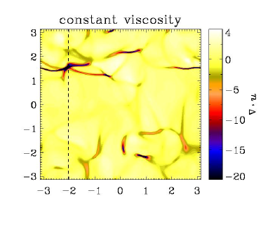
Figure 1: Grey scale (colour scale in electronic version) representation of $\mbox{\boldmath$\nabla$}{}\cdot{\bm{u}}$ in an $xy$ cross-section through $z=0$ for $\mbox{\rm Ma}=1.1$ using constant viscosity (upper panel: Run 3a, $512^{3}$ meshpoints) and shock-capturing viscosity (lower panel: Run 3b, $128^{3}$ meshpoints). Both simulations have been run from an initial state with zero velocity, to a state where the kinetic energy has saturated, but the magnetic energy is still in the linear regime (i.e. there is no back reaction on the velocity). Note the drastic difference between the two regarding the sharpness of regions of strong convergence. In both panels, the dotted line indicates the position of the scan shown in Fig. 2.

Figure 2: Value of $\mbox{\boldmath$\nabla$}{}\cdot{\bm{u}}$ along a line through the box whose position is indicated in Fig. 1. Here $\mbox{\rm Ma}=1.1$ and we are comparing constant viscosity (solid line) and shock-capturing viscosity (dashed line).

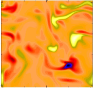
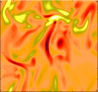
Figure 3: Same as Fig. 1, but for ${\bm{B}}_{z}$. Left figure is from a run with $512^{3}$ meshpoints and normal viscosity while right figure is from a run with $128^{3}$ meshpoints and shock viscosity. Since this is in the linear regime we have normalized by the rms value. There is surprisingly little difference between the two.

Figure 4: Probability distribution function of $B_{x}$, $B_{y}$ and $B_{z}$, normalized by $B_{\rm rms}$, for Run 3a (upper panel) and Run 3b (lower panel).

Figure 5: The different terms in the induction equation for Run 3a (with $512^{3}$ mesh points and constant viscosity). We clearly see that the dominant term is the advection term.

We make a more detailed comparison of two equivalent simulations, one with and one without shock viscosity. In each of the two cases the Mach number is the same, e.g. $\mbox{\rm Ma}\approx 1.1$, $f_{0}=0.5$. Corresponding cross-sections of $\mbox{\boldmath$\nabla$}{}\cdot{\bm{u}}$ are shown in Fig. 1. In the direct simulations the regions with $\mbox{\boldmath$\nabla$}{}\cdot{\bm{u}}<0$ are quite sharp, compared with the shock-capturing simulations where they are smoother. This is seen more clearly in Fig. 2 where we plot $\mbox{\boldmath$\nabla$}{}\cdot{\bm{u}}$ along a cross-section (shown as a dashed line in Fig. 1). Since the runs are turbulent, however, direct comparison between individual structures is meaningless and one can only make qualitative comparisons.

The number of strong convergence regions and shocks is roughly similar in both cases, but this is only because we have used the same grey/colour scale in both plots. In the direct simulation, the dynamical range is $-62\leq\mbox{\boldmath$\nabla$}{}\cdot{\bm{u}}\leq 4.2$, which exceeds the range of the grey/colour scale, whereas in the shock-capturing simulation the dynamical range is only $-17\leq\mbox{\boldmath$\nabla$}{}\cdot{\bm{u}}\leq 4.2$. If one were to compare the two cases such that in each the grey/colour scale is exactly within the dynamical range of that simulation, one would see more structures in the shock-capturing simulation.

The dynamo-generated magnetic fields are generally rather smooth in both cases and in that respect rather similar to each other; see Fig. 3. Indeed, the filling factors where the field exceeds its rms value are similar in the two cases (0.09 in the left hand panel for the direct simulation simulation and 0.13 in the right hand panel for the shock capturing simulation). The probability density functions of the three components of the magnetic field are in both cases stretched exponentials (Fig. 4), which is in agreement with earlier results (Brandenburg et al., 1996).

In order to elucidate the reason for the almost complete absence of any shock-like structures in the dynamo-generated magnetic field, we show in Fig. 5 the different contributions to the right hand side of $\partial B_{z}/\partial t$ for Run 3a with normal viscosity. The grey/colour scale is the same in all panels. It is evident that the dominant term in the induction equation is the advection term, $-{\bm{u}}\cdot\mbox{\boldmath$\nabla$}{}B_{z}$. The stretching term, ${\bm{B}}\cdot\mbox{\boldmath$\nabla$}{}u_{z}$, gives the weakest contribution. The compression term, $-B_{z}\mbox{\boldmath$\nabla$}{}\cdot{\bm{u}}$, gives an intermediate contribution, but, more importantly, there are only a few barely noticeable contributions from shocks. This is mainly because in the locations of the shocks (for example at $x\approx-1.5$ $y\approx 2$; see upper panel of Fig. 1) the normal component of the magnetic field is weak (Fig. 3), making the shocks less pronounced in the product of the two (i.e. in $B_{z}\mbox{\boldmath$\nabla$}{}\cdot{\bm{u}}$). The end result is a relatively weak contribution to the right hand side of $\partial B_{z}/\partial t$.

In the cross-sections of the current density we see very similar structures in the simulations with normal and shock capturing viscosities; see Fig. 6. This is supported by the filling factors which are $\approx 0.1$ for both the left and the right hand sides of the figure.

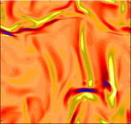
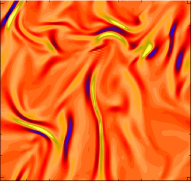
Figure 6: Same as Fig. 3, but for ${\bm{J}}_{z}$. Since this is in the linear regime we have normalized by the rms value. The current sheets are similar in thickness, but there are more of them in the shock-capturing simulation.

In Fig. 7 we plot the critical magnetic Reynolds number $\mbox{\rm Re}_{\rm M,crit}$ as a function of Mach number. It turns out that the critical magnetic Reynolds number increases from about 35 in the subsonic regime to about 70 in the supersonic regime. Whether or not the critical magnetic Reynolds number increases even further for larger Mach numbers is unclear, because larger resolution is required to settle this question for $\mbox{\rm Pr}_{M}=1$. However, in the direct simulations with $\mbox{\rm Pr}_{M}=5$ (Fig. 8), and in the shock-capturing simulations with $\mbox{\rm Pr}_{M}=1$ the critical magnetic Reynolds number is roughly unchanged when Ma is increased beyond $\mbox{\rm Ma}\approx 1$. We refer to this possibility of having two distinct values of the critical magnetic Reynolds number for subsonic and supersonic turbulence, with a reasonably sharp transition at $\mbox{\rm Ma}\approx 1$, as ‘bimodal’ behaviour.

Comparing direct and shock-capturing simulations we find the general appearance of the cross-sections of ${\bm{B}}$ remarkably similar. The simulations with shock-capturing viscosity have, however, slightly larger critical magnetic Reynolds numbers. This is probably explained by the smaller velocity gradients and hence smaller stretching rates in the simulations with additional shock-capturing viscosity. Nevertheless, both direct and shock-capturing simulations show a roughly similar functional dependence of the critical magnetic Reynolds number on the Mach number. This suggests that shock-capturing simulations provide a reasonable approximation to the much more expensive direct simulations–at least as far as the onset of turbulent dynamo action is concerned.

Figure 7: Critical magnetic Reynolds number $\mbox{\rm Re}_{\rm M,crit}$ as a function of Ma for simulations with $\mbox{\rm Pr}_{M}=1$. Note that $\mbox{\rm Re}_{\rm M,crit}$ depends strongly on Mach number for $\mbox{\rm Ma}\approx 1$. The simulations with shock-capturing viscosity give approximately the correct growth rates. The simulations that provide these data points have resolutions ranging from $64^{3}$ to $512^{3}$ mesh points. (Some of them are listed in Table 1.)

Figure 8: Same as Fig. 7 but for simulations with $\mbox{\rm Pr}_{M}=5$.

Once the Mach number becomes comparable to unity, one needs very high resolution to resolve the rather thin shock structures. However, as seen above, the magnetic field structures are by far not as thin as the hydrodynamic shocks. This implies that one can decrease $\eta$ to values far below $\nu$ before the magnetic field and current structures would become unresolved. In other words, with given resolution, one can reach a magnetic Reynolds number that is much larger than the kinematic Reynolds number. Alternatively, if one only wants to reach just weakly supercritical values of $\mbox{\rm Re}_{M}$ for dynamo action (which turn out to be roughly below one hundred), Re can be much smaller and just a few tens. This regime corresponds to large values of $\mbox{\rm Pr}_{M}$. For $\mbox{\rm Pr}_{M}=5$, for example, we are able to reach Mach numbers of up to 2.1. The resulting plot of $\mbox{\rm Re}_{\rm M,crit}$ versus Ma is shown in Fig. 8. This plot confirms again the approximately ‘bimodal’ behaviour of the critical magnetic Reynolds number, but now $\mbox{\rm Re}_{\rm M,crit}\approx 25$ in the subsonic regime and $\mbox{\rm Re}_{\rm M,crit}\approx 50$ in the supersonic regime.

Figure 9: Energy spectra for Runs 1a and 1c. The dotted lines give the result using shock-capturing viscosity (numbers in parentheses in the table).

The kinetic and magnetic energy spectra show close agreement between the constant and shock-capturing viscosity solutions at low wavenumbers; see Fig. 9. The truncation at higher wavenumbers is presumably a direct consequence of the locally enhanced shock viscosity which attempts to increase the width of the shocks. Furthermore, since shocks hardly manifest themselves in the magnetic field, the agreement between the magnetic energy spectra in the direct and shock-capturing simulations extends to even larger wavenumbers. As discussed in the beginning of Sect. 3, the direct simulations require vastly more resolution, but once the resolution is sufficient, either of the two spectra agrees well when doubling the resolution; see also the middle panel of Fig. 13 in Haugen et al. (2004).

4 Discussion

The present results have shown that in both direct and shock-capturing simulations the onset of dynamo action requires a somewhat larger magnetic Reynolds number when the Mach number exceeds a critical value around unity. In the subsonic regime the critical magnetic Reynolds number for nonhelical dynamo action is around 35, but it increases to about 70 in the supersonic regime. Once the Mach number exceeds unity, the critical magnetic Reynolds number no longer seems to depend on the Mach number. This confirms the notion that in the supersonic regime dynamos experience an additional sink. This additional sink is plausibly related to the sweeping up of magnetic field by shocks, but this effect does not gain in its importance with increasing Mach number once we are already in the supersonic regime.

The relative importance of the adverse effects of shocks can be associated with a Reynolds number-like quantity

$$R_{{\rm div}\,{}{\bm{u}}}=\left.\langle(\mbox{\boldmath$\nabla$}{}\cdot{\bm{u}})^{2}\rangle^{1/2}\right/\left(\nu k_{\rm f}^{2}\right),$$ (11)

whose dependence on the actual Reynolds number is shown in Fig. 10. Here we also compare with a similar number quantifying the relative importance of vortical motions,

$$R_{\omega}=\left.\langle\mbox{\boldmath$\omega$}{}^{2}\rangle^{1/2}\right/\left(\nu k_{\rm f}^{2}\right).$$ (12)

Both numbers seem to approach a limiting behaviour proportional to $\mbox{\rm Re}^{1.2}$. On theoretical grounds, one would have expected a slope of 3/2, because the ratio of rms velocity to rms vorticity is proportional to the Taylor microscale which, in turn, is known to diminish proportional to $\mbox{\rm Re}^{-1/2}$. The departure from this expectation might indicate that we are not yet in the asymptotic regime with a well developed inertial range. This is also plausible from Fig. 9 showing that most of the spectrum is dominated by a rather extended dissipative subrange with only a rather short inertial range. Thus, it might not be surprising that the Taylor microscale does not yet show a clear asymptotic $\mbox{\rm Re}^{-1/2}$ scaling.

Figure 10: Dependence of $R_{{\rm div}\,{}{\bm{u}}}$ and $R_{\omega}$ on Re. Note that both quantities remain well separated as they tend to approach a slope of 1.2.

Figure 10 suggests that $R_{{\rm div}\,{}{\bm{u}}}$ remains smaller than $R_{\omega}$ by a constant factor of around 1.5. Thus, $\langle(\mbox{\boldmath$\nabla$}{}\cdot{\bm{u}})^{2}\rangle/\langle\mbox{\boldmath$\omega$}{}^{2}\rangle\approx 0.44$. This ratio would be exactly 1/2 if the mean square values of longitudinal and transversal velocity derivatives were equal, i.e. $\langle u_{x,x}^{2}\rangle=\langle u_{x,y}^{2}\rangle$. Here we have assumed isotropy and that mixed terms cancel, which implies $\langle(\mbox{\boldmath$\nabla$}{}\cdot{\bm{u}})^{2}\rangle\approx 3\langle u_{x,x}^{2}\rangle$ and $\langle\mbox{\boldmath$\omega$}{}^{2}\rangle\approx 6\langle u_{x,y}^{2}\rangle$, giving a ratio of $1/2$.

Obviously, it will be important to confirm the asymptotic behaviour of $R_{\omega}^{2}/R_{{\rm div}\,{}{\bm{u}}}^{2}$ at larger Reynolds and Mach numbers and to relate this to the value of the critical magnetic Reynolds number for dynamo action. At the moment our simulations are simply limited by the resolution ($512^{3}$ meshpoints) which in turn is limited by the computing power available on modestly big supercomputers. Even though somewhat larger resolutions are already possible ($1024^{3}$ meshpoints), those runs remain prohibitively expensive if one needs to run for many turnover times.

Although we have here focused on the critical value of the magnetic Reynolds number for dynamo action, rather than the growth rate, we can see that there is currently no evidence for an increasing growth rate with increasing Mach number. From Runs 1a and 3a in Table 1, one sees that, as Ma increases from 0.72 to 1.1, the growth rate actually decreases, even though the magnetic Reynolds number is the same. By comparison, early work on small scale dynamo action in irrotational turbulence (Kazantsev et al., 1985) has shown that the growth rate should increase with the Mach number to the fourth power. Although we cannot confirm this, it is important to bear in mind that irrotational turbulence is not likely to correspond to the limit of large Mach numbers. Instead, as discussed above, the irrotational contribution to the flow velocity may converge to a finite fraction of the total flow velocity in the limit of large Mach numbers.

5 Conclusions

The present simulations suggest that the critical magnetic Reynolds number for the onset of dynamo action switches from about 35 in the subsonic regime to about 70 in the supersonic regime, and stays then approximately constant (at least in the range $1.0\leq\mbox{\rm Ma}\leq 2.6$ that we were able to simulate). It turns out that the simulations with shock-capturing viscosity yield almost the same critical magnetic Reynolds number as the direct simulations. This is partly explained by the fact that the shock structures are approximately equally smooth for both direct and shock-capturing viscosities. Finally, we note that there is as yet no support for the expectation that the growth rate is proportional to the Mach number to the fourth power, as was suggested previously by analytic theory assuming that the flow is irrotational (Kazantsev et al., 1985; Moss & Shukurov, 1996). It is suggested that this is because supersonic turbulence cannot accurately be described as being fully irrotational. Indeed, we find that the Reynolds number based on the vortical component of the flow is always larger than the Reynolds number based on the irrotational component.

In order to verify the proposed asymptotic independence of the critical magnetic Reynolds number on the Mach number, it would be useful to extend both the direct and the shock-capturing simulations to larger values of the Mach number. An obvious reason why this may not have been done yet is that when shock capturing viscosities are used, one normally uses at the same time also a similarly defined shock-capturing magnetic diffusivity. Consequently, a definition of the usual magnetic Reynolds number is no longer possible, and the connection between effective magnetic Reynolds number (based on the shock-capturing magnetic diffusivity) and the actual one is unclear. This is why in the present work we kept the magnetic diffusivity and the kinematic viscosity equal to the microscopic one. Even when we compared with shock-capturing simulations, the magnetic diffusivity was still kept constant. In conclusion, we feel that the use of shock-capturing viscosities in dynamo simulations with constant magnetic diffusivities provides a reasonable tool for investigating supersonic hydromagnetic turbulence.

References

- de Avillez & Mac Low (2002) Avillez, M. A., & Mac Low, M.-M. 2002, ApJ, 581, 1047
- Balsara et al. (2004) Balsara, D. S., Kim, J. K. Mac Low, M. M., & Mathews, G., 2004 Generation of magnetic fields in the multi-phase ISM with supernova-driven turbulence (astro-ph/0403660
- Bykov (1988) Bykov, A. M. 1988, Sov. Astron. Lett., 14, 60
- Brandenburg et al. (1996) Brandenburg, A., Jennings, R. L., Nordlund, Å., Rieutord, M., Stein, R. F., & Tuominen, I. 1996, JFM, 306, 325
- Haugen et al. (2003) Haugen N. E. L., Brandenburg A., & Dobler W. 2003, ApJ, 597, L141
- Haugen et al. (2004) Haugen N. E. L., Brandenburg A., & Dobler W. 2004, PRE, 69, astro-ph/0405453
- Kadomtsev & Petviashvili (1973) Kadomtsev B. B., & Petviashvili V. I. 1973, Sov. Phys. Dokl., 18, 115
- Kazantsev et al. (1985) Kazantsev A. P., Ruzmaikin A. A., & Sokoloff D. D. 1985, Sov. Phys. JETP, 88, 487
- Korpi et al. (1999) Korpi M. J., Brandenburg A., Shukurov A., Tuominen I., and Nordlund Å 1999, ApJ, 514, L99
- Moss & Shukurov (1996) Moss D., & Shukurov A. 1996, MNRAS, 279, 229
- Nordlund & Galsgaard (1995) Nordlund, Å., & Galsgaard, K. 1995, A 3D MHD code for Parallel Computers (http://www.astro.ku.dk/~aake/NumericalAstro/papers/kg/mhd.ps.gz)
- Padoan et al. (1997) Padoan P., Nordlund Å, & Jones B. J. T. 1997, ApJ, 288, 145
- Padoan & Nordlund (1999) Padoan P., & Nordlund Å 1999, ApJ, 526, 279
- Padoan & Nordlund (2002) Padoan, P., & Nordlund, Å. 2002, ApJ, 576, 870
- Padoan et al. (2004) Padoan, P., Jimenez, R., Nordlund, Å., & Boldyrev, S. 2004, PRL, 92, 191102
- Porter et al. (1998) Porter D. H., Woodward P. R., & Pouquet A. 1998, Phys. Fluids, 10, 237
- Richtmyer & Morton (1967) Richtmyer, R. D., Morton, K. W. 1967, Difference methods for initial-value problems (John Wiley & Sons)
- Roettiger et al. (1999) Roettiger K., Stone J. M., & Burns J. O. 1999, ApJ, 518, 594
- Zakharov & Sagdeev (1970) Zakharov V. E., & Sagdeev R. Z. 1970, Sov. Phys. Dokl., 15, 439