A kinetic control of the heliospheric interface hydrodynamics of charge-exchanging fluids

It is well known that the Solar System is presently moving through a partially ionized local interstellar medium. This gives rise to a counter-flow situation requiring a consistent description of behaviour of the two fluids – ions and neutral atoms – which are dynamically coupled by mutual charge exchange processes. Solutions to this problem have been offered in the literature, all relying on the assumption that the proton fluid, even under evidently nonequilibrium conditions, can be expected to stay in a highly-relaxated distribution function given by mono-Maxwellians shifted by the local proton bulk velocity. Here we check the validity of this assumption, calculating on the basis of a Boltzmann-kinetic approach the actually occurring deviations. As we show, especially for low degrees of ionization, $\xi\leq 0.3$, both the H-atoms and protons involved do generate in the heliospheric interface clearly pronounced deviations from shifted Maxwellians with asymmetrically shaped distribution functions giving rise to non-convective transport processes and heat conduction flows. Also in the inner heliosheath region and in the heliotail deviations of the proton distribution from the hydrodynamic one must be expected. This sheds new light on the correctness of current calculations of H-atom distribution functions prevailing in the inner heliosphere and also of the Lyman-$\alpha$ absorption features in stellar spectra due to the presence of the hydrogen wall atoms. Deviations from LTE-functions would be even more pronounced in magnetic interfaces, which via CGL-effects cause temperature anisotropies to arise.

1 Introduction

The problem of the heliospheric interface, where H-atoms and protons are effectively coupled by charge exchange interactions, has often been faced in the literature. In general, it was recognized very early that the passage of neutral interstellar atoms (O, H) through the plasma interface ahead of the solar wind termination shock needs a kinetic treatment, since the relevant charge exchange mean free paths between H-atoms and protons are comparable to or even larger than the typical structure scales of the interface plasma flow (i.e., Knudsen numbers are equal to or smaller than 1; see Ripken & Fahr 1983; Fahr & Ripken 1984; Fahr 1991; Osterbart & Fahr 1992; Baranov & Malama 1993 ; McNutt et al., 1998, Bzowski et al. 2000; Izmodenov et al. 2001) . Nevertheless, due to mathematical complications associated with such kinetic treatments of the problem, many heliospheric models have appeared in the literature which use hydrodynamic treatments of the two fluids, H-atoms and protons, coupled by charge exchange reactions (for recent reviews, see Zank 1999; Fahr 2003b).

The hydrodynamics applied in all these approaches is restricted to the description of the space-time behavior of the lowest hydrodynamic moments like density, bulk velocity and pressure and the local distribution function is taken to be solely a function of these moments in the form of shifted Maxwellians. As suggested in Fig.1, the permanent supply of newly charge-exchanged particles into the local distribution functions will maintain the resulting distribution (shown by dashed lines) far from a three-moment HD distribution.

This has been clearly recognized by Baranov and Malama (1993, 1995), who for this reasons perfected a kinetic treatment for the neutral H-atoms, even in view of the mathematical complications. The semi-kinetic approach offered by them, though treating the H-atom kinetically, is still based on the assumption that the protons can be described as a hydrodynamic fluid. But this is not true under special conditions, as we will demonstrate here. The protons generate deviations from a 3-moment HD-distribution. Therefore to represent the two fluids interacting by charge exchange reactions one would need a kinetic description both for the H-atoms and the protons. This highly complicated model will not be offered in this paper, but we present calculations which clearly make visible the resulting deviations of H-atom and proton distributions from 3-moment HD distributions. One other point, which was already emphasized by Fahr (2003a,b), concerns the fact that hydrodynamic two-fluid descriptions of the interface flows use charge-exchange coupling terms which are only justified in cases of supersonic bulk velocity differences. Under realistic interface conditions the resulting bulk velocity differences, however, appear to have subsonic magnitudes and thus require revised formulations of the charge exchange coupling terms. In the following we thus subject hydrodynamic approaches to a kinetic control.

2 Theoretical approach

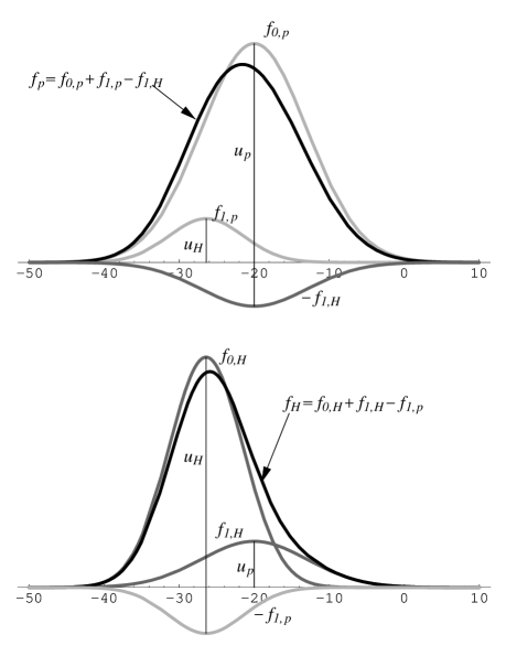
Figure 1: Schematic view of the “old” proton and H-atom distribution functions ($f_{0,p}$ and $f_{0,H}$, light gray and dark gray, respectively), with different bulk velocities $u_{p}$, $u_{H}$ and temperatures, interacting with each other by charge exchange. The charge exchange gives rise to secondary populations of protons and H-atoms that inherit the kinematic properties of their respective source populations of unperturbed H-atoms and protons. As a result, non-Maxwellian distribution functions $f_{p}$, $f_{H}$ of both protons and H-atoms appear, shown in black lines.

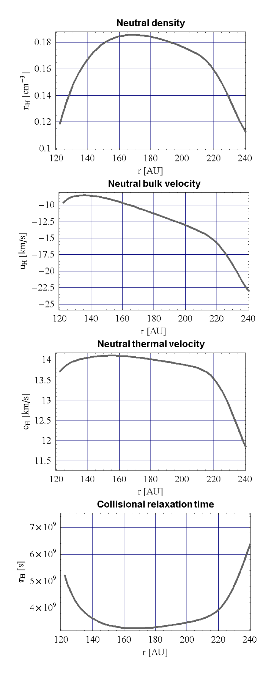
Figure 2: Macroscopic parameters of H-atoms between the bow shock and the heliopause, calculated with the use of the multi-fluid hydrodynamical treatment developed by Fahr et al. (2000). The bow shock is at $\sim 250$ AU, the heliopause at $\sim 125$ AU.

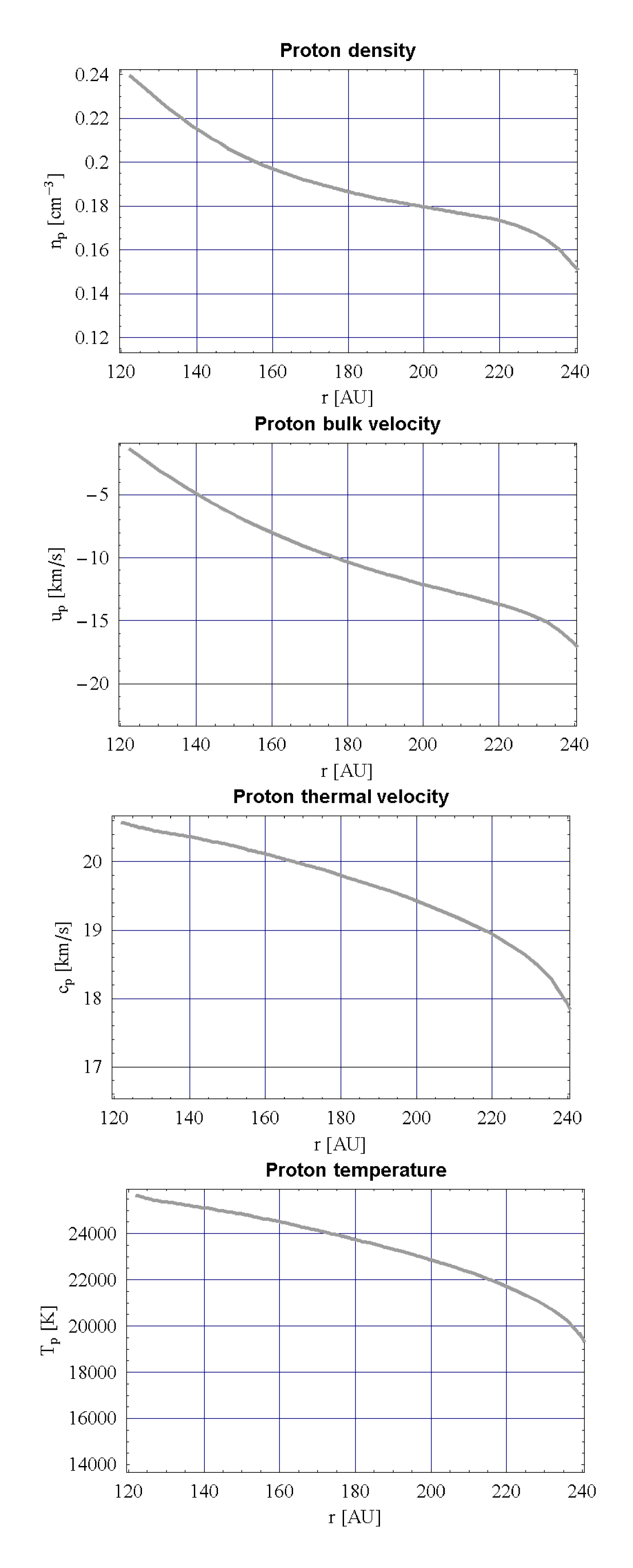
Figure 3: Macroscopic parameters of protons between the bow shock and the heliopause, calculated with the use of the multi-fluid hydrodynamical treatment developed by Fahr et al. (2000).

We assume that protons and hydrogen atoms in the interface are coupled solely by charge exchange processes. For simplicity, we limit ourselves to calculations on the stagnation line only. Denoting the hydrogen distribution function by $f_{H}$ and the proton distribution function by $f_{p}$ we furthermore assume that the two distribution functions can be represented by Maxwellian cores $f_{0,H}$, $f_{0,p}$ from hydrodynamic calculations and by non-relaxed corrections $f_{1,H}$, $f_{1,p}$ due to mutual implantations of new charge exchanged particles, as shown in the following formulae and qualitatively in Fig.1:

$$f_{H}\left(\@vec{v},s\right)=f_{0,H}\left(\@vec{v},s\right)+f_{1,H}\left(\@vec{v},s\right)$$ (1)

$$f_{p}\left(\@vec{v},s\right)=f_{0,p}\left(\@vec{v},s\right)+f_{1,p}\left(\@vec{v},s\right)$$ (2)

where $s$ measures the spatial position on the symmetry axis. At this symmetry axis, and for stationary conditions, we have the following system of Boltzmann-kinetic equations in phase space, which couple the protons and hydrogen atoms via mutual losses and gains (see, e.g., Fahr 1996):

$$v\cos\theta\leavevmode\nobreak\ \frac{df_{H}}{ds}=\frac{\delta^{+}f_{H}}{\delta t}-\frac{\delta^{-}f_{H}}{\delta t}+\frac{f_{0,H}-f_{H}}{\tau_{H}}$$ (3)

$$v\cos\theta\leavevmode\nobreak\ \frac{df_{p}}{ds}=\frac{\delta^{+}f_{p}}{\delta t}-\frac{\delta^{-}f_{p}}{\delta t}+\frac{f_{0,p}-f_{p}}{\tau_{p}}$$ (4)

In these equations $s$ is a line element along the axis in the interface and $\tau_{H}$, $\tau_{p}$ are relaxation times, separate for protons and hydrogen atoms and dependent on $s$ and the particle velocities. The terms with $\delta^{+}$ and $\delta^{-}$ are, correspondingly, the production and loss terms, as shown in formulae 2 and 2, and the remaining terms in Eqs 3 and 4 are the relaxation terms operating to restitute the hydrodynamic solutions for appropriate distribution functions. The actually resulting distribution function $f$ which, had the local charge exchange influences been stopped, would relax towards the hydrodynamic core distribution $f_{0}$ within one relaxation period. But as long as charge exchange is operating, the resulting distribution is permanently kept off this function $f_{0}$. In other words, we assume that two-fluid hydrodynamics would deliver correct results in the interface had the H-atom and proton relaxation processes operated fast enough, i.e., if $\tau_{H},\,\tau_{p}<<\tau_{ex}$, $\tau_{ex}$ being the charge exchange period between the H-atoms and protons. Only because $\tau_{H},\,\tau_{p}\simeq\tau_{ex}$ deviations from the hydrodynamic core functions are pronounced. The above system of differential equations is valid for an arbitrary velocity vector $\@vec{v}\left(v,\cos\theta\right)$ but for a proton velocity vector identical to the H atom velocity vector. $\theta$ is the angle between the direction of atom’s motion and the inflow axis $z$ (and consequently $v\cos\theta=v_{z}$). No matter what the forms of the distribution functions are, a phase-space hydrogen gain is then a phase-space proton loss and vice versa. Hence equations 3 and 4 are modified to

$$v\cos\theta\leavevmode\nobreak\ \frac{df_{H}}{ds} = \frac{\delta^{-}f_{p}}{\delta t}-\frac{\delta^{-}f_{H}}{\delta t}-\frac{f_{1,H}}{\tau_{H}}$$ (5)

$$v\cos\theta\leavevmode\nobreak\ \frac{df_{p}}{ds} = \frac{\delta^{-}f_{H}}{\delta t}-\frac{\delta^{-}f_{p}}{\delta t}-\frac{f_{1,p}}{\tau_{p}}$$ (6)

Specifically, the two remaining coupling terms are of the following forms:

$$\frac{\delta^{-}f_{H}}{\delta t} = f_{H}\left(v,s,\theta_{H}\right)\times$$

$$\times \int v_{rel}\left(v,v_{p},\theta_{p}\right)\leavevmode\nobreak\ f_{p}\left(s,v_{p},\theta_{p}\right)\leavevmode\nobreak\ \sigma\left(v_{rel}\right)\leavevmode\nobreak\ d^{3}v_{p}$$

$$\frac{\delta^{-}f_{p}}{\delta t} = f_{p}\left(v,s,\theta_{p}\right)\times$$

$$\times \int v_{rel}\left(v,v_{H},\theta_{H}\right)\leavevmode\nobreak\ f_{H}\left(s,v_{H},\theta_{H}\right)\leavevmode\nobreak\ \sigma\left(v_{rel}\right)\leavevmode\nobreak\ d^{3}v_{H}$$

Here $v_{rel}\left(v,v_{p},\theta_{p}\right)$ denotes the relative velocity between an H-atom of velocity $v$ and a proton of velocity $v_{p}$ inclined at an angle $\theta_{p}$ to the proton bulk speed $\@vec{u}_{p}$. $\sigma\left(v_{rel}\right)$ is the H-atom – proton charge exchange cross section for particles with a relative velocity $v_{rel}$.

The core functions $f_{0,H/p}$ in the integrands will be taken from a hydrodynamic multifluid simulation code (Fahr et al. 2000) describing the interface system. They are functions of $s$ and defined as follows

$$f_{0,H}\left(v,s,\theta_{H}\right) = \left(\frac{1}{\pi\leavevmode\nobreak\ c_{H}}\right)^{\frac{3}{2}}\leavevmode\nobreak\ n_{H}\times$$

$$\times \exp\left[-\frac{v^{2}+u_{H}^{2}-2u_{H}\leavevmode\nobreak\ v\leavevmode\nobreak\ \cos\theta_{H}}{c_{H}^{2}\leavevmode\nobreak\ }\right]$$

$$f_{0,p}\left(v,s,\theta_{p}\right) = \left(\frac{1}{\pi\leavevmode\nobreak\ c_{p}}\right)^{\frac{3}{2}}\leavevmode\nobreak\ n_{p}\times$$

$$\times \exp\left[-\frac{v^{2}+u_{p}^{2}-2u_{p}\leavevmode\nobreak\ v\leavevmode\nobreak\ \cos\theta_{p}}{c_{p}^{2}\leavevmode\nobreak\ }\right]$$

where $u_{H}$, $u_{p}$ are, respectively, the local bulk velocities of hydrogen atoms and protons, which depend on the position and thus here are given as functions of the path length $s$ measured between the outer shock and the heliopause; $n_{H}$, $n_{p}$ are number densities, also dependent on $s$; $\theta_{H}$, $\theta_{p}$ are angles between the local bulk velocities, which of course on the axis must be parallel to the inflow axis, and the individual velocity $\@vec{v}$; and $c_{H}$, $c_{p}$ are thermal velocities of the core hydrogen atoms and protons, also dependent on $s$ via temperatures $T_{H}$, $T_{p}$:

$$c_{H}^{2}=\frac{2K\leavevmode\nobreak\ T_{H}\left(s\right)}{m}=\frac{2}{m}\frac{P_{H}\left(s\right)}{n_{H}\left(s\right)}$$ (11)

$$c_{p}^{2}=\frac{2K\leavevmode\nobreak\ T_{p}\left(s\right)}{m}=\frac{2}{m}\frac{P_{p}\left(s\right)}{n_{p}\left(s\right)}$$ (12)

We assume that the proton mass $m$ is equal to the hydrogen mass. The temperatures are also functions of $s$. In Figures 2 and 3 we present the core hydrodynamic quantities (density, bulk velocity, thermal velocity, and temperature) as functions of $s$, as they result from the multi-fluid interaction code developed by Fahr et al. (2000), which here was run for the following input parameters: solar wind speed: 400 km/s, solar wind density at 1 AU: 5 cm^-3, solar wind temperature at 1 AU: $10^{5}$ K, interstellar gas speed: 26 km/s, interstellar proton density: 0.1 cm^-3, interstellar hydrogen atom density: 0.1 cm^-3, interstellar gas temperature: 8000 K. The influences of pick-up ions and of anomalous and regular components of cosmic rays were switched off in this modelling for consistency with our kinetic approach presented in this paper, where couplings to these particle populations are not taken into account.

We thus start from a two-fluid hydrodynamic interface model in which H-atoms are represented by one single fluid only. This is different from modellings like that presented by Zank et al. (1996), where neutral hydrogen is decribed by three different fluids representing H-atoms a) coming directly from the interstellar medium, b) originating in the heliosheath, and c) originating in the inner heliosphere. For our approach here, where we want to check on kinetic deviations from hydrodynamic H-atom fluid approximations, we consider it to be more practical to start from a simple mono-Maxwellian representation of the H-atoms, thereby making our concept logically more convincing.

We rewrite the coupling terms defined in equations 2 and 2 so that the core + correction form of the distribution function (see Eq.1 and 2) is taken into account:

$$\frac{\delta^{-}f_{H}}{\delta t} = f_{H}\left(\@vec{v},s,\theta_{H}\right)\times$$

$$\times \left(\int v_{rel}\left(\@vec{v},\@vec{v}_{p}\right)f_{0,p}\left(s,\@vec{v}_{p}\right)\sigma\left(v_{rel}\right)d^{3}v_{p}+\right.$$

$$+ \left.\int v_{rel}\left(\@vec{v},\@vec{v}_{p}\right)f_{1,p}\left(s,\@vec{v}_{p}\right)\sigma\left(v_{rel}\right)d^{3}v_{p}\right)$$

$$\frac{\delta^{-}f_{p}}{\delta t} = f_{p}\left(\@vec{v},s,\theta_{p}\right)\times$$

$$\times \left(\int v_{rel}\left(\@vec{v},\@vec{v}_{H}\right)f_{0,H}\left(s,\@vec{v}_{H}\right)\sigma\left(v_{rel}\right)d^{3}v_{H}+\right.$$

$$+ \left.\int v_{rel}\left(\@vec{v},\@vec{v}_{H}\right)f_{1,H}\left(s,\@vec{v}_{H}\right)\sigma\left(v_{rel}\right)d^{3}v_{H}\right)$$

and then we neglect the correction terms in the integrals, since they only contribute according to their partial densities with $n_{1,H}\ll n_{0,H}$, $n_{1,p}\ll n_{0,p}$. We assume that the total density $n_{1}$ given by $f_{1}$ is negligible with respect to the total density $n_{0}$ given by $f_{0}$. This does not mean that $f_{1}$ itself is everywhere small with respect to $f_{0}$, as shown in Fig.1, where velocity regions where $f_{1}\geq f_{0}$ can be seen. We thus assume that in Eqs. 2 and 2 only terms $\left(f_{0,i}+f_{1,i}\right)\int f_{0,j}...$ must be taken into account. Hence only the shifted Maxwellians stay in the integrands of equations 2 and 2, yielding:

$$\frac{\delta^{-}f_{H}}{\delta t} = f_{H}\left(\@vec{v},s,\theta_{H}\right)\times$$

$$\times \int v_{rel}\left(\@vec{v},\@vec{v}_{p}\right)\leavevmode\nobreak\ f_{0,p}\left(s,\@vec{v}_{p}\right)\leavevmode\nobreak\ \sigma\left(v_{rel}\right)\leavevmode\nobreak\ d^{3}v_{p}$$

$$\frac{\delta^{-}f_{p}}{\delta t} = f_{p}\left(\@vec{v},s,\theta_{p}\right)\times$$

$$\times \int v_{rel}\left(\@vec{v},\@vec{v}_{H}\right)\leavevmode\nobreak\ f_{0,H}\left(s,\@vec{v}_{H}\right)\leavevmode\nobreak\ \sigma\left(v_{rel}\right)\leavevmode\nobreak\ d^{3}v_{H}$$

The validity of this assumption can be checked aposteriori in the results presented in Figures 5 through 8. It can be seen that close to the heliopause this assumption is violated.

The dependence of the charge exchange cross section on the relative velocity of colliding particles can be described by the well-known formula given by Maher & Tinsley (1977):

$$\sigma(v_{rel})=(A+B\log(v_{rel}))^{2},$$ (17)

where $A=1.6\,10^{-7}$ and $B=-6.8\,10^{-9}$. Now we further simplify, by assuming that the charge exchange cross section can be expanded into a constant + linear expansion term, i.e., expanding around the bulk velocity $\@vec{u}_{p}$ of the protons and bulk velocity $\@vec{u}_{H}$ of the H-atoms, respectively:

$$\sigma_{p}\left(\@vec{v}_{rel,p}\right) = \sigma_{0,p}+\sigma_{1,p}\left(\@vec{v}_{rel,p}-\@vec{v}_{0}\right)$$ (18)

$$\sigma_{H}\left(\@vec{v}_{rel,H}\right) = \sigma_{0,H}+\sigma_{1,H}\left(\@vec{v}_{rel,H}-\@vec{v}_{0}\right)$$ (19)

We take as $\@vec{v}_{0}$ appropriate bulk velocities $\@vec{u}_{p}$, $\@vec{u}_{H}$ and we change variables so that now we will be in a reference system co-moving with the protons or vice versa with the hydrogen atoms. The coefficients $\sigma_{0}$ and $\sigma_{1}$ in equations 18 and 19 are calculated from the following formulae:

$$\sigma_{0,H}=\left(A+B\log\bar{u}_{H}\right)^{2}$$ (20)

$$\sigma_{1,H}=\frac{d\sigma}{dv}\left(\bar{u}_{H}\right)=2\left(A+B\log\bar{u}_{H}\right)\frac{B}{u_{H}}$$ (21)

$$\sigma_{0,p}=\left(A+B\log\bar{u}_{p}\right)^{2}$$ (22)

$$\sigma_{1,p}=\frac{d\sigma}{dv}\left(u_{p}\right)=2\left(A+B\log\bar{u}_{p}\right)\frac{B}{u_{p}}$$ (23)

where $\bar{u}_{p}$, $\bar{u}_{H}$ are velocities normalized by the velocity of 1 cm/s. The relative velocity $\@vec{v}_{rel}$ in equations 18 and 19 is expressed as $\@vec{v}_{rel,p}=\left|\@vec{u}_{p}-\@vec{v}\right|$ for protons and as $\@vec{v}_{rel,H}=\left|\@vec{u}_{H}-\@vec{v}\right|$ for hydrogen atoms.

In the co-moving reference systems the Maxwellian core distribution functions are the following:

$$f_{0,p}\left(v^{\prime},s\right) = \frac{n_{p}\left(s\right)}{\left(\pi\leavevmode\nobreak\ c_{p}\left(s\right)\right)^{3/2}}\exp\left[-\frac{v^{\prime 2}}{c_{p}\left(s\right)^{2}}\right]$$ (24)

$$f_{0,H}\left(v^{\prime},s\right) = \frac{n_{H}\left(s\right)}{\left(\pi\leavevmode\nobreak\ c_{H}\left(s\right)\right)^{3/2}}\exp\left[-\frac{v^{\prime 2}}{c_{H}\left(s\right)^{2}}\right]$$ (25)

where $v^{\prime}$ are specific velocities in the appropriate co-moving frames. Evaluating equations 2 and 2 with the use of 18, 19 brings the following expressions for the coupling terms:

$$\frac{\delta^{-}f_{H}}{\delta t} = f_{H}\left[\sigma_{0,p}\int v_{rel,p}\leavevmode\nobreak\ f_{0,p}\leavevmode\nobreak\ d^{3}v_{p}^{\prime}+\right.$$

$$+ \left.\sigma_{1,p}\int v_{rel,p}^{2}\leavevmode\nobreak\ f_{0,p}\leavevmode\nobreak\ d^{3}v_{p}^{\prime}\right]$$

$$\frac{\delta^{-}f_{p}}{\delta t} = f_{p}\left[\sigma_{0,H}\int v_{rel,H}\leavevmode\nobreak\ f_{0,H}\leavevmode\nobreak\ d^{3}v_{H}^{\prime}+\right.$$

$$+ \left.\sigma_{1,H}\int v_{relH}^{2}\leavevmode\nobreak\ f_{0,H}\leavevmode\nobreak\ d^{3}v_{H}^{\prime}\right]$$

The relative velocities under the integrands are defined as follows:

$$v_{rel,p}^{2}=v^{2}+u_{p}^{2}-2v\leavevmode\nobreak\ u_{p}\leavevmode\nobreak\ \cos\theta$$ (28)

$$v_{rel,H}^{2}=v^{2}+u_{H}^{2}-2v\leavevmode\nobreak\ u_{H}\leavevmode\nobreak\ \cos\theta$$ (29)

From Fahr & Mueller (1967) and Ripken & Fahr (1983), the mean relative velocities coming out from the first integral in equations 2 and 2 are given by formulae:

$$\left\langle v_{rel,p}\right\rangle=\frac{c_{p}}{\sqrt{\pi}}\exp\left[-\frac{u_{p}^{2}}{c_{p}^{2}}\right]+u_{p}\left(1+\frac{c_{p}}{2u_{p}}\right){\rm erf}\left(\frac{u_{p}}{c_{p}}\right)$$ (30)

$$\left\langle v_{rel,H}\right\rangle=\frac{c_{H}}{\sqrt{\pi}}\exp\left[-\frac{u_{H}^{2}}{c_{H}^{2}}\right]+u_{H}\left(1+\frac{c_{H}}{2u_{H}}\right){\rm erf}\left(\frac{u_{H}}{c_{H}}\right)$$ (31)

For the second integral in formulae 2 and 2, we notice that the integration over $\theta$ will bring to 0 the terms with $\cos\theta$ and that – since $u_{p}$, $u_{H}$ are local quantities which do not depend on $v$ – the second term from the relative velocity expansion (equations 28 and 29) will simply yield $u_{p}^{2}$ times the result of integration of the core distribution function over the velocity space. We therefore can denote this result simply by $n_{0,H}$ and $n_{0,p}$, respectively. The remaining integrations of the mean square velocity with respect to the core distribution functions yield simply the local thermal velocities and thus finally the integrations defined in equations 2 and 2 lead to the following results:

$$\frac{\delta^{-}f_{H}}{\delta t}=n_{p}\leavevmode\nobreak\ f_{H}\leavevmode\nobreak\ \left[\sigma_{0,p}\left\langle v_{rel,p}\right\rangle+\sigma_{1,p}\left(u_{T,p}^{2}+u_{p}^{2}\right)\right]$$ (32)

$$\frac{\delta^{-}f_{p}}{\delta t}=n_{H}\leavevmode\nobreak\ f_{p}\leavevmode\nobreak\ \left[\sigma_{0,H}\left\langle v_{rel,H}\right\rangle+\sigma_{1,H}\left(u_{T,H}^{2}+u_{H}^{2}\right)\right]$$ (33)

with the mean relative velocities defined in Equations 30 and 31. The set of differential equations, originally defined by formulae 3 and 4, is now obtained in the following form:

$$v\cos\theta\frac{df_{1,H}}{ds} = -v\cos\theta\frac{df_{0,H}}{ds}-\frac{f_{1,H}}{\tau_{H}}-n_{p}\left(f_{0,H}+f_{1,H}\right)\times$$

$$\times \left[\sigma_{0,p}\left\langle v_{rel,p}\right\rangle+\sigma_{1,p}\left(c_{p}^{2}+u_{p}^{2}\right)\right]+$$

$$+ n_{H}\left(f_{0,p}+f_{1,p}\right)\times$$

$$\times \left[\sigma_{0,H}\left\langle v_{rel,H}\right\rangle+\sigma_{1,H}\left(c_{H}^{2}+u_{H}^{2}\right)\right]$$

$$v\cos\theta\frac{df_{1,p}}{ds} = -v\cos\theta\frac{df_{1,p}}{ds}-\frac{f_{1,p}}{\tau_{p}}-n_{H}\left(f_{0,p}+f_{1,p}\right)\times$$

$$\times \left[\sigma_{0,H}\left\langle v_{rel,H}\right\rangle+\sigma_{1,H}\left(c_{H}^{2}+u_{H}^{2}\right)\right]+$$

$$+ n_{p}\left(f_{0,H}+f_{1,H}\right)\times$$

$$\times \left[\sigma_{0,p}\left\langle v_{rel,p}\right\rangle+\sigma_{1,p}\left(c_{p}^{2}+u_{p}^{2}\right)\right]$$

The above equations can be rewritten so that the terms multiplied by $f_{1,p;H}$ are collected together:

$$v\cos\theta\frac{df_{1,H}}{ds} = -v\cos\theta\leavevmode\nobreak\ \frac{df_{0,H}}{ds}-\frac{f_{1,H}}{\tau_{H}}-$$

$$- f_{1,H}n_{p}\,\left(\sigma_{0,p}\left\langle v_{rel,p}\right\rangle+\sigma_{1,p}\left(c_{p}^{2}+u_{p}^{2}\right)\right)+$$

$$+ f_{1,p}\leavevmode\nobreak\ n_{H}\left[\sigma_{0,H}\left\langle v_{rel,H}\right\rangle+\sigma_{1,H}\left(c_{H}^{2}+u_{H}^{2}\right)\right]-$$

$$- f_{0,H}\leavevmode\nobreak\ n_{p}\left[\sigma_{0,p}\left\langle v_{rel,p}\right\rangle+\sigma_{1,p}\left(c_{p}^{2}+u_{p}^{2}\right)\right]+$$

$$+ f_{0,p}\leavevmode\nobreak\ n_{H}\left[\sigma_{0,H}\left\langle v_{rel,H}\right\rangle+\sigma_{1,H}\left(c_{H}^{2}+u_{H}^{2}\right)\right]$$

$$v\cos\theta\frac{df_{1,p}}{ds} = -v\cos\theta\leavevmode\nobreak\ \frac{df_{0,p}}{ds}-\frac{f_{1,p}}{\tau_{p}}-$$

$$- f_{1,p}n_{H}\left(\sigma_{0,H}\left\langle v_{rel,H}\right\rangle+\sigma_{1,H}\left(c_{H}^{2}+u_{H}^{2}\right)\right)+$$

$$+ f_{1,H}\leavevmode\nobreak\ n_{p}\left[\sigma_{0,p}\left\langle v_{rel,p}\right\rangle+\sigma_{1,p}\left(c_{p}^{2}+u_{p}^{2}\right)\right]-$$

$$- f_{0,p}\leavevmode\nobreak\ n_{H}\left[\sigma_{0,H}\left\langle v_{rel,H}\right\rangle+\sigma_{1,H}\left(c_{H}^{2}+u_{H}^{2}\right)\right]+$$

$$+ f_{0,H}\leavevmode\nobreak\ n_{p}\left[\sigma_{0,p}\left\langle v_{rel,p}\right\rangle+\sigma_{1,p}\left(c_{p}^{2}+u_{p}^{2}\right)\right]$$

These equations hence formally represent the following linear system of differential equations:

$$v\cos\theta\frac{df_{1,H}}{ds} = A\left(s\right)+B\left(s\right)\leavevmode\nobreak\ f_{1,H}+C\left(s\right)\leavevmode\nobreak\ f_{1,p}$$ (38)

$$v\cos\theta\frac{df_{1,p}}{ds} = D\left(s\right)+E\left(s\right)\leavevmode\nobreak\ f_{1,H}+F\left(s\right)\leavevmode\nobreak\ f_{1,p}$$ (39)

with the multiplicative factors $A,B,C,D,E,F$ defined as follows:

$$A\left(s\right) = -v\cos\theta\leavevmode\nobreak\ \frac{df_{0,H}}{ds}-$$

$$-f_{0,H}\leavevmode\nobreak\ n_{p}\left[\sigma_{0,p}\left\langle v_{rel,p}\right\rangle+\sigma_{1,p}\left(c_{p}^{2}+u_{p}^{2}\right)\right]+$$

$$+f_{0,p}\leavevmode\nobreak\ n_{H}\left[\sigma_{0,H}\left\langle v_{rel,H}\right\rangle+\sigma_{1,H}\left(c_{H}^{2}+u_{H}^{2}\right)\right]$$

$$B\left(s\right) = -\left[\frac{1}{\tau_{H}}+n_{p}\left(\sigma_{0,p}\left\langle v_{rel,p}\right\rangle+\sigma_{1,p}\left(c_{p}^{2}+u_{p}^{2}\right)\right)\right]$$ (41)

$$C\left(s\right) = n_{H}\left[\sigma_{0,H}\left\langle v_{rel,H}\right\rangle+\sigma_{1,H}\left(c_{H}^{2}+u_{H}^{2}\right)\right]$$ (42)

$$D\left(s\right) = -v\cos\theta\leavevmode\nobreak\ \frac{df_{0,p}}{ds}+$$

$$+f_{0,H}\leavevmode\nobreak\ n_{p}\left[\sigma_{0,p}\left\langle v_{rel,p}\right\rangle+\sigma_{1,p}\left(c_{p}^{2}+u_{p}^{2}\right)\right]-$$

$$-f_{0,p}\leavevmode\nobreak\ n_{H}\left[\sigma_{0,H}\left\langle v_{rel,H}\right\rangle+\sigma_{1,H}\left(c_{H}^{2}+u_{H}^{2}\right)\right]$$

$$E\left(s\right) = n_{p}\left[\sigma_{0,p}\left\langle v_{rel,p}\right\rangle+\sigma_{1,p}\left(c_{p}^{2}+u_{p}^{2}\right)\right]$$ (44)

$$F\left(s\right) = -\frac{1}{\tau_{p}}-n_{H}\left(\sigma_{0,H}\left\langle v_{rel,H}\right\rangle+\sigma_{1,H}\left(c_{H}^{2}+u_{H}^{2}\right)\right)$$ (45)

The derivatives of the unperturbed distribution functions given by Equation 2 and 2 are calculated as follows:

$$\frac{df_{0,H}}{ds}=\frac{\partial f_{0,H}}{\partial n_{H}}\leavevmode\nobreak\ \frac{dn_{H}}{ds}+\frac{\partial f_{0,H}}{\partial u_{H}}\leavevmode\nobreak\ \frac{du_{H}}{ds}+\frac{\partial f_{0,H}}{\partial c_{H}}\leavevmode\nobreak\ \frac{dc_{H}}{ds}$$ (46)

and analogously for the function $f_{0,p}$. The terms of equation 46 are evaluated as follows:

$$\frac{\partial f_{0,H}}{\partial n_{H}}=\frac{f_{0,H}}{n_{H}}$$ (47)

$$\frac{\partial f_{0,H}}{\partial u_{H}}=-2f_{0,H}\frac{u_{H}-v\leavevmode\nobreak\ \cos\theta}{c_{H}^{2}}$$ (48)

$$\frac{\partial f_{0,H}}{\partial c_{H}}=\frac{f_{0,H}}{c_{H}}\left(2\frac{v^{2}+u_{H}^{2}-2v\leavevmode\nobreak\ u_{H}\leavevmode\nobreak\ \cos\theta}{c_{H}^{2}}-\frac{3}{2}\right)$$ (49)

Collecting them all together we obtain the following expression for the derivatives of the unperturbed distribution functions:

$$\frac{df_{0,H}}{ds} = f_{0,H}\left[\frac{\frac{dn_{H}}{ds}}{n_{H}}-\frac{2}{c_{H}^{2}}\left(\left(u_{H}-v\cos\theta\right)\frac{du_{H}}{ds}-\right.\right.$$

$$- \left.\left.\left(\frac{v^{2}+u_{H}^{2}-2vu_{H}\leavevmode\nobreak\ \cos\theta}{c_{H}}-\frac{3}{4}\right)\frac{dc_{H}}{ds}\right)\right]$$

$$\frac{df_{0,p}}{ds} = f_{0,p}\left[\frac{\frac{dn_{p}}{ds}}{n_{p}}-\frac{2}{c_{p}^{2}}\left(\left(u_{p}-v\leavevmode\nobreak\ \cos\theta\right)\frac{du_{p}}{ds}-\right.\right.$$

$$- \left.\left.\left(\frac{v^{2}+u_{p}^{2}-2v\leavevmode\nobreak\ u_{p}\leavevmode\nobreak\ \cos\theta}{c_{p}}-\frac{3}{4}\right)\frac{dc_{p}}{ds}\right)\right]$$

Now we need the relaxation times, used in equations 5 and 6. For the relaxation of the neutral hydrogen gas, the only mechanism is elastic H – H collisions. The corresponding relaxation time is numerically given by Brinkmann (1970) and Fahr (1996) in the following form:

$$\tau_{H}=\frac{6.62\cdot 10^{10}}{n_{H}\sqrt{T_{H}}}=\frac{6.62\cdot 10^{10}}{n_{H}\leavevmode\nobreak\ c_{H}}\sqrt{\frac{2K}{m}}=\frac{8.51\cdot 10^{14}}{n_{H}\leavevmode\nobreak\ c_{H}}\leavevmode\nobreak\ {\rm s}$$ (52)

for $n_{H}$ expressed in cm^-3 and $c_{H}$ in cm/s. The period $\tau_{H}$ turns out to be very long in comparison to charge exchange periods $\tau_{ex}$, i.e., $\tau_{H}/\tau_{ex}\simeq 10$. The relaxation time for protons is more difficult to calculate. If, however, the secondary protons have a bulk velocity small enough to not be shifted outside the broad thermal envelope of the “hydrodynamic” proton population (in other words, the net distribution function does not feature two distinct peaks), then the wave-particle interaction by a two-stream instability should not be significant. If, in addition, the pre-existing turbulence level in the unperturbed LIC is small at the distance scale comparable to and smaller than the size of the interface, then also non-linear interaction with MHD waves (mainly Alfvén waves) may be negligible and the only relaxation mechanism will be Coulomb collisions between the old and newly-created protons. A more in-depth discussion will be presented in Sec.4 at the end of this paper.

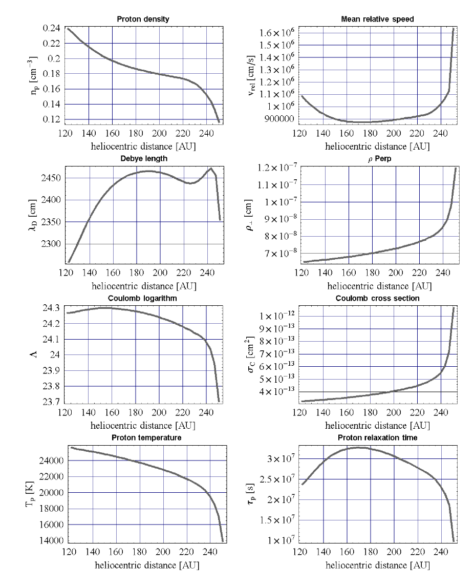
Figure 4: Parameters relevant to compute the proton relaxation time, discussed in Eq. 53 through 61, as functions of the heliocentric distance between the bowshock and the heliopause, based on the parameters shown in Fig. 3.

The proton relaxation time is defined as the time between Coulomb collisions of a proton traveling at $v$ and protons belonging to the core population, described by the proton distribution function $f_{0}$ being a Maxwellian shifted by $u_{p}$ with thermal velocity $c_{p}$, and is obtained from the mean free path with respect to Coulomb collisions $\lambda_{C}$ in the form:

$$\tau_{p}=\frac{\lambda_{C}}{v_{rel,p}}=\frac{1}{\frac{1}{2}n_{p}\leavevmode\nobreak\ \sigma_{C}\leavevmode\nobreak\ \left\langle v_{rel,p}\right\rangle}$$ (53)

where $\frac{1}{2}$ is the energy transfer efficiency term, equal to the reduced mass of the colliding particles: $2\,m_{p}\leavevmode\nobreak\ m_{p}/\left(m_{p}+m_{p}\right)^{2}$.

The angle-averaged mean momentum-transfer Coulomb collision cross section $\sigma_{C}$ in Eq. 53 is given by the textbook formula (e.g., Oraevskij 1989):

$$\sigma_{C}=\sigma_{C,\perp}\Lambda$$ (54)

where $\Lambda$ is the Coulomb logarithm defined as

$$\Lambda=\ln\frac{\lambda_{D}}{\rho_{\perp}}$$ (55)

$\sigma_{C,\perp}$ is defined by the formula:

$$\sigma_{C,\perp}=\pi\rho_{\perp}^{2}$$ (56)

and $\rho_{\perp}$ in Eq.56 is defined by

$$\frac{e^{2}}{\rho_{\perp}}=K\leavevmode\nobreak\ T_{p}$$ (57)

thus yielding

$$\rho_{\perp}=\frac{e^{2}}{K\leavevmode\nobreak\ T_{p}}$$ (58)

so consequently

$$\sigma_{C,\perp}=\frac{\pi e^{4}}{\left(K\leavevmode\nobreak\ T_{p}\right)^{2}}$$ (59)

In Eqs 54 through 59 $K$ is Boltzmann constant; $\left\langle v_{rel,p}\right\rangle$ is the mean relative velocity of the test particle (the newly-created proton) with respect to the unperturbed proton population described by $f_{0,p}$, defined in Eq. 30; and $e$ is the cgs elementary charge. Deep inside the interface, at 200 AU from the Sun, the proton density $n_{p}=0.18$ cm^-3, proton temperature $T_{p}=2.3\leavevmode\nobreak\ 10^{4}$ K, and the relative speed $\left\langle v_{rel,p}\right\rangle=9\leavevmode\nobreak\ 10^{5}$ cm/s. In Eq.55 $\lambda_{D}$ is the Debye length, defined by the formula:

$$\lambda_{D}=\sqrt{\frac{KT_{p}}{4\pi\leavevmode\nobreak\ n_{p}\leavevmode\nobreak\ e^{2}}}=c_{p}\sqrt{\frac{m}{8\pi\leavevmode\nobreak\ n_{p}\leavevmode\nobreak\ e^{2}}}=6.9\sqrt{\frac{T_{p}}{n_{p}}}$$ (60)

which for the above-mentioned conditions in the heliospheric interface is equal to $\sim$2460 cm, and the Coulomb logarithm $\Lambda$, defined in Eq. 55, to $\sim$24.25. Thus the total Coulomb cross section $\sigma_{C}$, defined in Eq.54, is equal to $\sim 4\leavevmode\nobreak\ 10^{-13}$ cm². Hence the proton relaxation time within the outer interface, at $\sim 200$ AU from the Sun, is of the order of a year:

$$\tau_{p}\simeq 3.1\leavevmode\nobreak\ 10^{7}{\rm s}$$ (61)

These times $\tau_{p}$ become even much larger in the inner interface and in the heliotail. These estimates may express the fact that relaxation processes are fairly unimportant here as well for the protons as especially for the H-atoms because the relaxation periods are comparable to the mean passage times or structuring times

$$\tau_{s}=\frac{n_{H,p}}{u_{H,p}\frac{dn_{H,p}}{ds}}\approx 10^{8}{\rm s}$$ (62)

In the final section of this paper we shall, however, come back to this point. The dependence of all the above referenced quantities on the axial coordinates counted along the axis in the interface is shown in Figs 4.

3 Results and discussion

We solved the system of equations 38, 39 (separarately for each $v$) using the hydrodynamic core distribution functions given in Eqs 2 and 2, with the parameters obtained from hydrodynamic simulations by Fahr et al. (2000) and shown in Figures 2 and 3. In the approach presented here, where H-atoms are represented by a mono-Maxwellian plus kinetic deviations, we can only represent solutions of the distribution function for positive values of H-atom velocities. In order to present solutions for negative values of H-atom velocities we would need to integrate Equs 3 and 4 in the opposite direction (negative increments of $s$!) starting from an inner boundary value for the H-atom distribution function $f_{0,H}\left(s_{0},-v_{H}\right)$. Since our hydrodynamic H-atom core functions vanish for negative velocity values, we cannot use any reasonable boundary condition to calculate the H-atom distribution functions for negative velocity values unless we admit additional H-atom fluids, as practised by Zank et al. (1996). The results for densities $n_{p,H}$, bulk velocities $u_{p,H}$, and temperatures $T_{p,H}$ have been calculated on the basis of the assumption that the underlying distribution functions $f_{p,H}$ are three-moment functions, i.e., shifted Maxwellians. In contrast, in the kinetic theory presented in this paper we have calculated those distribution functions actually occurring in the outer interface under the action of charge exchange processes between the locally colliding H-atoms and protons. These results we show in Figures 5 through 8. In these figures we have displayed at several interface positions on the symmetry axis one-dimensional cuts through the kinetically resulting distribution functions $f_{p,H}$, showing both the unperturbed hydrodynamical distribution functions $f_{0(p,H)}$ and the kinetically perturbed, actually resulting distribution functions $f_{(p,H)}=f_{0(p,H)}+f_{1(p,H)}$.

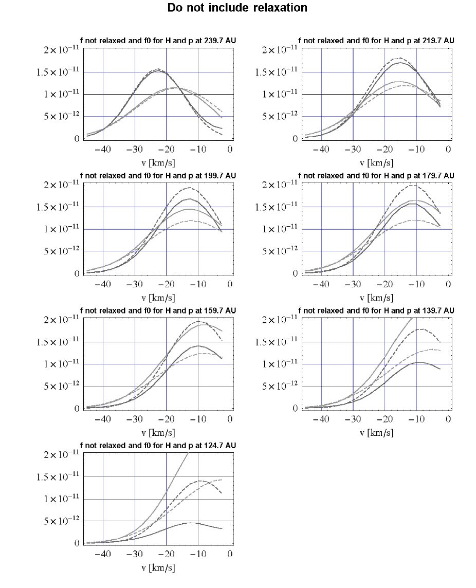
Figure 5: Hydrogen and proton distribution functions: no proton relaxation case. Light gray lines correspond to protons and dark gray to H-atoms. Shown at selected distances from the Sun (in the region between the bow shock and the heliopause) are the unperturbed Maxwellian distribution functions, drawn with broken lines, and the net distribution functions $f_{p;H}=f_{0,p;H}+f_{1,p;H}$, drawn with the solid lines and expressed in atoms cm^-6 s^-3.

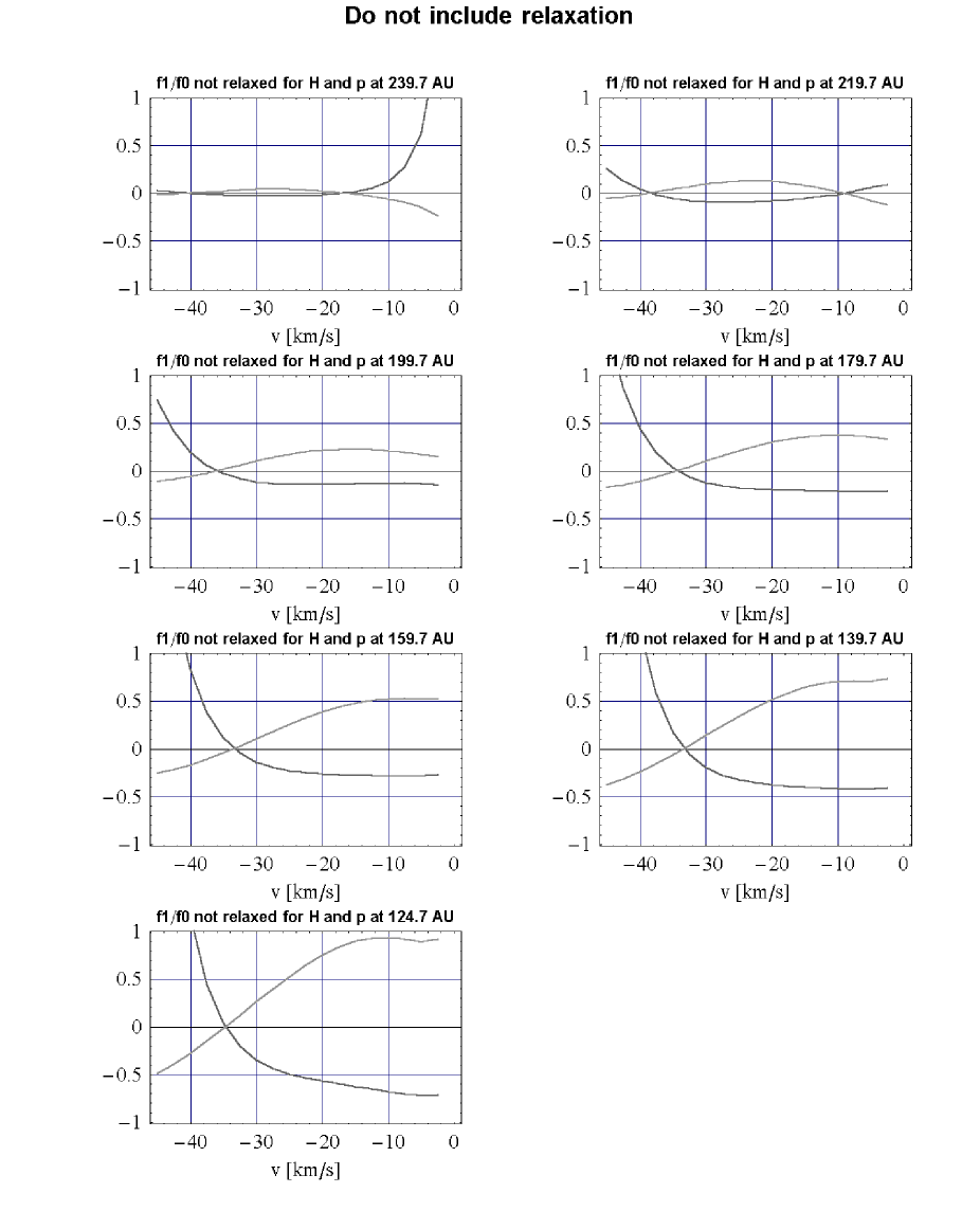
Figure 6: Ratios of the perturbation functions $f_{1,p;H}$ to the corresponding unperturbed distribution functions $f_{0,p;H}$: the $f_{1}/f_{0}$ ratios, in the case of no proton relaxation operating, drawn for the H-atoms in dark gray and for the protons in light gray.

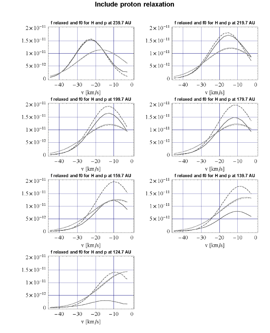
Figure 7: Hydrogen and proton distribution functions: proton Coulomb relaxation case. Light gray lines correspond to protons and dark gray to H-atoms. Shown at selected distances from the Sun (in the region between the bow shock and the heliopause) are the unperturbed Maxwellian distribution functions, drawn with broken lines, and the net distribution functions $f_{p;H}=f_{0,p;H}+f_{1,p;H}$, drawn with the solid lines and expressed in atoms cm^-6 s^-3.

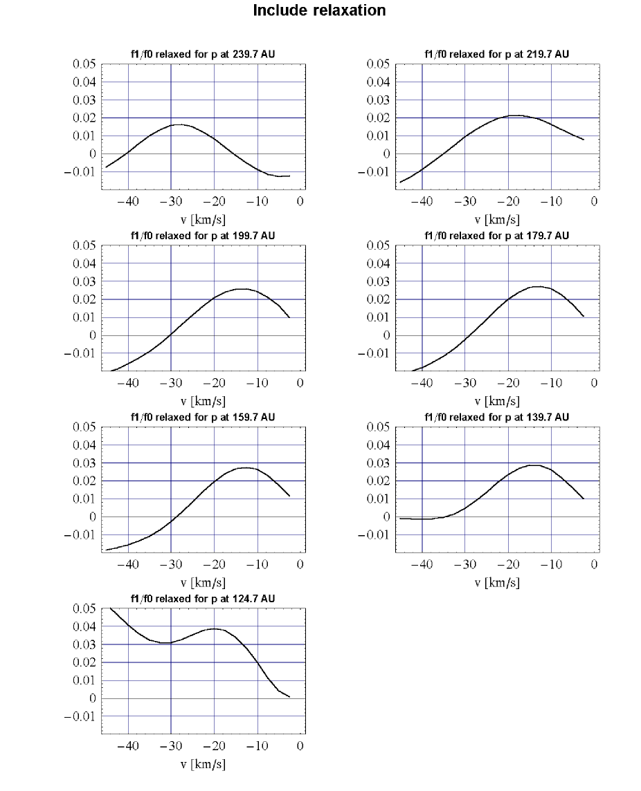
Figure 8: Ratios of the proton perturbation function to the proton unperturbed distribution function: $f_{1}/f_{0}$ for the proton Coulomb relaxation operating.

First in Fig. 5 we display $v_{z}$-cuts through the distribution functions $f_{H}$ and $f_{p}$ resulting at various positions $s=s_{i}$ in the interface, when proton-proton relaxation processes are suppressed, but atom-atom relaxation processes are working. As one can clearly see, pronounced deviations of both resulting distribution functions $f_{(p,H)}$ from simple shifted Maxwellians, derived by hydrodynamical studies, can be recognized. These are even better identifiable in Fig. 6, where we have displayed the ratios $f_{1(p,H)}/f_{0(p,H)}$. Switching on the proton-proton Coulomb collision relaxation, as developed in Eq. 53 and as shown in Figs 7 and 8, reduces these deviations in the case of proton distribution functions to much milder degrees. Thus, under LISM conditions as used here in this paper, the hydrodynamically derived distribution functions for the interface protons may be considered as good approximations, whereas the hydrodynamic approach to the H-atom distribution definitely is a poor approximation. Thus, due to rapid relaxation processes under the conditions adopted in this paper deviations of protons from hydrodynamically derived Maxwellians can be considered as fairly small.

In contrast, however, if interfaces for different LISM conditions need to be modelled, a kinetic revision of such proton distribution functions becomes necessary. For instance, this would be the case for lower LISM proton densities, because the proton-proton relaxation rate/period drastically goes down/up. For example, a LISM proton density of $n_{p,\infty}=0.01$ cm^-3 would increase the relaxation rate by more than a factor of 10 with respect to the one used here, thus meaning in consequence that non-relaxated proton distribution functions must be expected. This would become important in the inner heliosheath and in the heliotail. This all the more will be true if magnetic fields control the interface MHD dynamics and by CGL-effects (Chew et al. 1956) may lead to pronounced temperature anisotropies.

As one can notice in Figs 7 and 8, the closer one approaches the Sun starting from the outer bow shock, the more the resulting kinetic distribution function $f_{(p,H)}$ deviates from the unperturbed hydrodynamic distribution $f_{0(p,H)}$, even reaching nonlinear amounts of such deviations. The specific form of these deviations thereby are not systematic with the coordinate $s$ and could only perhaps be studied in more detail by the analysis of the higher moments of the distribution function $f_{(p,H)}$, like the heat conduction flow or the temperature anisotropies. Qualitatively at least one can say – as it was already anticipated in the qualitative results sketched in Fig. 1 – that the solar/antisolar wings of the distributions $f_{(p,H)}$ are enhanced with respect to the unperturbed ones $f_{0(p,H)}$, wherever the local bulk velocities $u_{(p,H)}$ are larger than those $u_{(p,H)}$. Under these conditions heat conduction flows result from the distribution functions $f_{(p,H)}$, which for protons are directed in the direction of $\@vec{u}_{H}-\@vec{u}_{p}$ and for H-atoms in the direction $\@vec{u}_{p}-\@vec{u}_{H}$.

This fact has two consequences for the modelling of the H-atom presence in the inner and outer heliosphere. One is that the distribution function $f_{H}$, which describes the injection of the LISM H-atoms into the inner heliosphere, is different from what was assumed up to now. This thus will influence the predictions made with respect to the H-atom phase-space distribution in the inner heliosphere and the related predictions on the resulting spectral and integrated Lyman-$\alpha$ resonance glow (see, e.g., Scherer et al. 1999). Another consequence may be that calculations of the absorption spectra caused by hydrogen atoms in the hydrogen wall ahead of the heliopause (see papers by Linsky & Wood 1996; Wood & Linsky 1997; Gayley et al. 1997; Izmodenov et al. 1999) may need revision. For instance, the asymmetric shapes of the resulting H-atom distribution function presented in this paper lead to asymmetric spectral absorption features at Lyman-$\alpha$ wavelengths which could remedy the problems in the correct representation of the observed stellar spectra (see, e.g., Izmodenov et al. 1999).

4 Outlook: Competing proton relaxation processes in heliospheric interface

In the above calculations we have made use of the assumption that relaxation of the actually formed proton distribution function towards an associated equilibrium distribution $f_{0}$ with $\delta\left(\int f_{0}\leavevmode\nobreak\ \ln f_{0}\leavevmode\nobreak\ d^{3}v\right)/\delta t=0$ operates on time scales comparable to charge exchange time scales and the typical interface passage times. As proton-proton relaxation processes we only have taken into account p-p Coulomb interaction. This assumption should be justified and for that purpose we are looking for some alternative processes which could support the relaxation of the proton distribution function.

Since the proton distribution function resulting in the interface is a consequence of charge-exchange induced interaction between the distributions of protons and H-atoms, the proton distribution function $f_{p}$ approximately represents a superposition of two shifted Maxwellians with different partial densities $n_{0}$ and $n_{1}$, the latter being due to ionized H-atoms. Under such circumstances it is suggestive to first investigate whether excitation of electron plasma waves by the positive slope of the composite distribution function may be an important contribution to a relaxation of such non-equilibrium distributions towards a best-adapted mono-Maxwellian.

Taking the approach presented by Davidson et al. (1970) and going to the limit of full equilibration of electron thermal and differential proton bulk energies, one obtains a friction force $R_{e,i}$ per unit volume acting between protons and electrons given by (see Fahr & Neutsch 1983):

$$R_{e,i}=J\gamma_{\max}W_{k0}\sqrt{\frac{m_{e}}{KT_{e}}}$$ (63)

where $J=39.9$ is found as a constant, $m_{e}$ and $T_{e}$ are the electron mass and temperature, respectively, $\gamma_{\max}$ is the maximum growth rate of the excited plasma waves (i.e., most unstable electrostatic mode) given by:

$$\gamma_{\max}=\omega_{p}\frac{\sqrt{3}}{2}\sqrt[3]{\frac{m_{e}}{4m_{p}}}$$ (64)

where $\omega_{p}$ is the electron plasma frequency, and $W_{k0}$ is the total wave power which according to Davidson et al. (1970) in the saturation phase attains the following value:

$$W_{k0}\simeq n_{e}m_{e}(u_{H}-u_{p})^{2}$$ (65)

where $u_{H}$ and $u_{p}$ are the z-components of the local bulk velocities of the H-atoms and the protons, respectively. The above mentioned friction force $R_{e,i}$ operates with the tendency to reduce the differential bulk kinetic energy in the proton distribution function. Thus one can derive a typical relaxation time $\tau_{e,i}$ with the following relation:

$$\ \tau_{e,i}\simeq\frac{n_{1}(\frac{1}{2}m_{p}(u_{H}-u_{p})^{2})}{R_{e,i}u_{p}}$$ (66)

Inserting values like $n_{0}=0.1$ cm^-3, $n_{1}/n_{0}=0.1$, $u_{H}=25$ km/s, $u_{p}=10$ km/s, and $KT_{e}=\frac{1}{4}m_{e}(u_{H}-u_{p})^{2}$ one gets the result: $\tau_{e,i}\simeq 2000$ s.

From the above estimate one should expect to have the relaxation of the non-equilibrium proton distribution occurring via electron plasma wave excitations within astonishingly short times $\tau_{e,i}$ of the order of one or a few hours.

One should, however, check the validity of the assumptions made in the above derivation of the time $\tau_{e,i}$. As it turns out, the results of Davidson et al. (1970) can in principle be adopted only if the two Maxwellian peaks in the superposed distribution function are clearly separated from each other and do not essentially overlap by their Maxwellian wings. When looking at the conditions which in fact are prevailing at least on the interstellar side of the heliospheric interface it becomes fairly evident that this condition is by far not fulfilled, since the proton thermal velocity is of the order of 20 km/s and the separation of the bulks only amounts to perhaps 15 km/s.

This conclusion can also be supported by looking into the Landau damping rates or the plasma oscillation growth rates $\gamma_{p}(\omega,k)$ which are connected to the derivatives with respect to $v_{z}$ of the normalized distribution function $f_{p,z}^{\times}=\int\int f_{p}^{\times}dv_{x}dv_{y}$ by the following relation:

$$\gamma_{p}(\omega,k)\simeq\frac{\omega_{p}^{3}}{\pi k^{2}}\left|\frac{\partial f_{p,z}^{\times}}{\partial v_{z}}\right|_{v_{z}=\omega/k}=\omega_{p}\frac{v_{z}^{2}}{\pi}\left|\frac{\partial f_{p,z}^{\times}}{\partial v_{z}}\right|_{v_{z}}$$ (67)

where the normalized distribution function $f_{p,z}^{\times}$ may approximately be represented by:

$$f_{p,z}^{\times}(w_{z}) \simeq \frac{1}{\sqrt{\pi}}\exp\left[-w_{z}^{2}\right]+\frac{1}{\sqrt{\pi}}\frac{n_{1}}{n_{0}}\left(\frac{T_{p}}{T_{H}}\right)^{1/2}\times$$

$$\times \exp\left[-\frac{T_{p}}{T_{H}}\left(W_{H}-W_{p}-w_{z}\right)^{2}\right]$$

Here the following denotations were used: $w_{z}^{2}=m_{p}v_{z}^{2}/(2KT_{p})$; $W_{H}^{2}=m_{p}u_{H}^{2}/(2KT_{p})$;  $W_{p}^{2}=m_{p}u_{p}^{2}/(2KT_{p})$; $T_{p}$ and $T_{H}$ are the temperatures of the bulk of the protons and of the H-atoms, respectively. Now from the above relations one finds:

$$\frac{\partial f_{p,z}^{\times}}{\partial w_{z}} \simeq \frac{-2w_{z}}{\sqrt{\pi}}\exp[-w_{z}^{2}]+\frac{2}{\sqrt{\pi}}\frac{n_{1}}{n_{0}}\left(\frac{T_{p}}{T_{H}}\right)^{3/2}\times$$

$$\times (W_{H}-W_{p}-w_{z})\exp\left[-\frac{T_{p}}{T_{H}}\left(W_{H}-W_{p}-w_{z}^{2}\right)\right]$$

The most positive contribution comes from the second hump in the distribution function to $f_{p,z}^{\times}(w_{z})$ and leads to positive growth rates evidently coming from regions of $w_{z}$ where the following relation is valid: $W_{H}-W_{p}-w_{z}\simeq 1$, which then leads to:

$$\left|\frac{\partial f_{p,z}^{\times}}{\partial w_{z}}\right|_{1} \simeq \frac{-2(W_{H}-W_{p}-1)}{\sqrt{\pi}}\exp\left[-(W_{H}-W_{p}-1)^{2}\right]+$$ (70)

$$+ \frac{2}{\sqrt{\pi}}\frac{n_{1}}{n_{0}}\left(\frac{T_{p}}{T_{H}}\right)^{3/2}\exp\left[-\frac{T_{p}}{T_{H}}\right]$$

Taking now typical values for the above quantities as they prevail in the LISM interface we can decide whether positive growth rates are possible. In view of the values we display in Figures 3 and 2 of Section 1 we select the following typical values: $W_{H}\simeq 3$; $W_{p}\simeq 0.3$; $T_{p}/T_{H}\simeq 12000/8000=1$, and thus:

$$\left|\frac{\partial f_{p,z}^{\times}}{\partial w_{z}}\right|_{1} \simeq \frac{-2(1.7)}{\sqrt{\pi}}\exp[-(1.7)^{2}]+\frac{2}{\sqrt{\pi}}\frac{n_{1}}{n_{0}}(1.5)^{\frac{3}{2}}{\rm e}^{-\frac{3}{2}}=\$$

$$= \frac{2}{\sqrt{\pi}}\exp[-(1.7)^{2}]\left(\frac{n_{1}}{n_{0}}(1.5)^{3/2}\exp\left[+0.2\right]-1\right)$$

meaning that only under unlikely conditions, not met in our calculations above and characterized by:

$$\frac{n_{1}}{n_{0}}\geq\frac{1}{1.5^{3/2}}\exp(-0.2)=0.44$$ (72)

a relaxation of the distribution function $f_{p,z}^{\times}$ by excitation of electron plasma waves is likely to occur.

It thus remains to inspect relaxation processes connected to the nonlinear interaction of protons with MHD turbulences, amongst which pitch angle diffusion processes seem to be the most effective ones. These, however, depend on the local magnetic fields and the existing MHD turbulence levels. Of course, nothing is known at present about LISM magnetic fields and turbulences. This is why no good estimate of pitch-angle diffusion processes is possible here as is otherwise feasible on the basis of an expression already derived by Hasselmann & Wibberenz (1970) in which the typical time period for pitch angle diffusion is given by:

$$\tau_{\parallel}\simeq\frac{\lambda_{\parallel}}{v}=\frac{3}{8}\int_{-1}^{+1}\frac{\left(1-\mu^{2}\right)^{2}d\mu}{D_{\mu\mu}},$$ (73)

where $\lambda_{\parallel}$ is the mean free path with respect to pitch-angle scattering, $\mu$ is the pitch angle cosine, and $D_{\mu\mu}$ is the Fokker-Planck pitch angle diffusion coefficient. The latter, however, is a complicated function of particle velocity, local magnetic field magnitudes, Alfvén velocities, and turbulence levels. This coefficient $D_{\mu\mu}$ then leads to velocity-dependent mean free paths $\lambda_{\parallel}(v)$ and to corresponding scattering periods $\tau_{\parallel}(v)$ (as given by Chalov & Fahr 1999a,b for keV-energetic ions). The needed input information to evaluate the above expression unfortunately are completely lacking for the LISM interface region and furthermore the newly injected ions from the H-atom population in this region only have energies of about 10 eV. Thus we cannot estimate $\tau_{\parallel}$ in this way.

Instead we estimate the relaxation times connected with pitch angle scattering on the basis of the reasonable expectation that the locally appearing MHD turbulence levels are not primarily due to convected pre-existing turbulences, which have not been quantitatively described in the literature, but due to wave-driving processes of secondary protons injected via charge exchange processes into an unstable mode of the proton distribution function. Let us assume that the newly created protons produced by charge exchange are populated in a region of velocity space where they represent some free kinetic energy by which they are able to drive some MHD wave power (see, e.g., Huddleston & Johnstone 1992, Williams & Zank 1994, Fahr & Chashei 2002). Let us then assume that this free energy is pumped into turbulent wave power essentially at an injection wave number $k_{i}$. The following considerations are of course only relevant if an interstellar magnetic field is present. For an unmagnetized interstellar medium what follows here would thus be irrelevant.

Adopting that near the symmetry axis (stagnation line!) a background magnetic field $B_{LISM}$ exists which is oriented parallel to the stagnation line (i.e., according to an MHD interaction model with $\@vec{B}_{LISM}\parallel\@vec{V}_{LISM}$ as treated, e.g., by Baranov & Zaitsev 1995, Pogorelov & Matsuda 1998, or Ratkiewicz & McKenzie 2003), one then can assume that Alfvén waves are excited by this free energy which then propagate upstream and downstream of the plasma flow. The free energy of newly injected protons stemming from the bulk of the H-atom distribution function can then be assumed to be pumped into the wave field at the injection wave number fulfilling the resonance conditions and given in the bulk plasma system by:

$$\mp k_{i}\simeq\Omega/\left(v_{A}\pm\left(u_{H}-u_{p}\right)\right)$$ (74)

Since hydromagnetic Alfvén waves have frequencies $\omega=v_{A}\ k\leq\Omega$ the cyclotron resonance condition can only be met by ions with positive/negative parallel velocities resonating with waves with negative/positive wave vectors. In the outer interface plasma newly injected ions with $u_{H}\geq u_{p}$ have positive parallel velocities in the plasma frame and thus can only resonate with waves propagating in the direction opposite to them with wave vector magnitudes $k_{i}\simeq\Omega/(v_{A}+(u_{H}-u_{p}))$. When resonating with these waves, energy can be exchanged between such ions and the waves up to an equilibrium situation. This injected wave power then cascades from $k_{i}$ to larger wave numbers described by a so-called wave-wave diffusion coefficient $D_{kk}$ (see Zhou & Matthaeus 1990) until the power arrives at a wave number $k_{dis}\simeq\Omega/v_{A}$ where it is resonantly absorbed by the bulk of the protons.

We now determine the time $\tau_{kk}$ needed to cascade the injected power to the dissipation wave scale – in order thereby to derive the time needed to transfer energy from the secondary proton hump in the proton distribution function to the primary proton bulk. Following Chashei et al. (2003) we obtain:

$$\tau_{kk}\simeq\frac{\left(\Delta k\right)^{2}}{4D_{kk}}=\frac{\left(k_{i}-k_{dis}\right)^{2}}{4D_{kk}}=\frac{\left(\frac{\Omega}{v_{A}+(u_{H}-u_{p})}-\frac{\Omega}{v_{A}}\right)^{2}}{4D_{kk}}$$ (75)

According to Zhou & Matthaeus (1990), we can represent the k-space diffusion coefficient by the following expression:

$$D_{kk}=Cv_{A}k_{i}^{7/2}\sqrt{\frac{4\pi W_{i}}{B_{LISM}}}$$ (76)

where $W_{i}$ denotes the spectral power at wave number $k_{i}$, and $C\simeq 0.1$ is a constant. Assuming that wave energy is injected at the same rate as it cascades down to $k_{dis}$, we can determine $W_{i}$ by the following relation:

$$W_{i}\Delta k\simeq\beta_{ex}\Delta\epsilon_{i}\tau_{kk}=\beta_{ex}\Delta\epsilon_{i}\frac{\Delta k^{2}}{4D_{kk}}$$ (77)

where $\beta_{ex}=n_{p}n_{H}\sigma_{ex}V_{rel}$ is the mean charge exchange rate between H-atoms and protons, and $\Delta\epsilon_{i}=\epsilon_{f}\left(\frac{1}{2}m_{p}\left(u_{H}-u_{p}\right)^{2}\right)$ is the free energy pumped from the newly injected protons into the wave field. With Eqs. (75) through (77) one thus finds:

$$W_{i}^{3/2}\simeq\frac{B_{LISM}}{2Cv_{A}k_{i}^{7/2}\sqrt{\pi}}\beta_{ex}\Delta\varepsilon_{i}\Delta k=\frac{\sqrt{\rho_{p}}\beta_{ex}\Delta\epsilon_{i}\Delta k}{Ck_{i}^{7/2}}$$ (78)

With the above result we finally find the diffusion time $\tau_{kk}$ as given by:

$$\tau_{kk} \simeq \frac{W_{i}\Delta k}{\beta_{ex}\Delta\epsilon_{i}}=\frac{\Delta k}{\beta_{ex}\Delta\epsilon_{i}}\left(\frac{\sqrt{\rho_{p}}\beta_{ex}\Delta\epsilon_{i}\Delta k}{4Ck_{i}^{7/2}}\right)^{2/3}=$$

$$= \frac{\left(\frac{u_{H}-u_{p}}{v_{A}}\right)^{5/3}}{2C^{2/3}\left(n_{H}\leavevmode\nobreak\ \sigma_{ex}V_{rel}\leavevmode\nobreak\ \epsilon_{f}\left(u_{H}-u_{p}\right)^{2}k_{i}^{2}\right)^{1/3}}$$

Let us now assume for estimation purposes that $V_{rel}$ can be reasonably well approximated by $V_{rel}\simeq(u_{H}-u_{p})$. Then we arrive at the following expression:

$$\tau_{kk} \simeq \frac{\left(u_{H}-u_{p}\right)^{2/3}}{2C^{2/3}v_{A}^{5/3}\left(n_{H}\leavevmode\nobreak\ \sigma_{ex}\leavevmode\nobreak\ \epsilon_{f}\leavevmode\nobreak\ k_{i}^{2}\right)^{1/3}}=$$

$$= \frac{\left(u_{H}-u_{p}\right)^{2/3}\left(v_{A}+u_{H}-u_{p}\right)^{2/3}}{2\epsilon_{f}^{1/3}C^{2/3\leavevmode\nobreak\ }v_{A}^{5/3}\leavevmode\nobreak\ \Omega^{2/3}\left(n_{H}\leavevmode\nobreak\ \sigma_{ex}\right)^{1/3}}$$

For further evaluation of this expression we transform it into the following form:

$$\tau_{kk}\simeq\frac{\left(X_{H}-X_{p}\right)^{2/3}\left(1+X_{H}-X_{p}\right)^{2/3}}{2\epsilon_{f}^{1/3}C^{2/3}\Omega^{2/3}\left(v_{A}\leavevmode\nobreak\ n_{H}\leavevmode\nobreak\ \sigma_{ex}\right)^{1/3}}$$ (81)

where the quantities $X_{H}$ and $X_{p}$ denote the corresponding bulk velocities normalized by $v_{A}$.

It remains to find some adequate value for the fraction $\epsilon_{f}$ of energy that is transferred as free energy to the wave fields. This value we intend to derive in analogy to a similar derivation given by Chashei et al. (2003) for the free energy of newly injected pick-up ions in the inner heliosphere. The following estimation cannot be carried out prior to at least some qualitative view of the configuration and magnitude of the magnetic field $B_{LISM}$ in the outer interface.

Hence we assume here that close to the stagnation line on the interstellar side of the interface we have a field $\@vec{B}_{{\rm LISM}}$ which is parallel to the plasma flow, i.e., parallel to $\@vec{u}_{p}$ (see, e.g., the model presented by Baranov & Zaitsev 1995). Then newly ionized H-atoms are implanted in the proton distribution function roughly at a velocity $\Delta u=\left|\@vec{u}_{H}-\@vec{u}_{p}\right|$ relative to the proton bulk flow. Injection of a newly created proton from the H-atom bulk on the average will eventually lead to the following relative velocity $g$ with respect to the proton bulk:

$$g\simeq\sqrt{\Delta u^{2}+c_{H}^{2}}$$ (82)

where $c_{H}$ is the thermal velocity of the H-atoms.

Now we consider the two frames of Alfvén waves moving with the velocity $\pm v_{A}$ relative to the proton bulk frame in up-field and down-field directions. With respect to these wave frames the injected protons have relative velocities given by:

$$g_{A\pm}=\sqrt{\left(v_{A}\pm\Delta u\right)^{2}+c_{H}^{2}}=\sqrt{v_{A}^{2}\pm 2v_{A}\leavevmode\nobreak\ \Delta u+g^{2}}$$ (83)

and by resonance with the up-field waves will rapidly be pitch-angle scattered onto the accessible spherical shell that is associated with the upgoing wave-frame (see Huddleston & Johnstone 1992). With respect to the proton bulk frame they thereby lose an energy $\Delta\epsilon_{f}$, taken as the pitch-angle average, given by (see Fahr & Chashei 2002, Chashei et al. 2003):

$$\Delta\epsilon_{f}\simeq\frac{1}{2}m_{p}\left[g^{2}-\left\langle g_{+}^{2}\left(\vartheta\right)\right\rangle\right]=\epsilon_{f}\left(\frac{1}{2}m_{p}\leavevmode\nobreak\ g^{2}\right)$$ (84)

where the angle-averaged velocity $\left\langle g_{+}^{2}(\vartheta)\right\rangle$ of the pitch-angle scattered new protons is given by:

$$\left\langle g_{+}^{2}\left(\vartheta\right)\right\rangle=\frac{\int\limits_{\cos\vartheta_{\max}^{\pm}}^{1}\left(v_{A}^{2}+g_{A+}^{2}-2v_{A}\leavevmode\nobreak\ g_{A\pm}\cos\vartheta\right)d\cos\vartheta}{1-\cos\vartheta_{\max}^{\pm}}$$ (85)

Here the maximum permitted inclination angles are defined by:

$$\cos\vartheta_{\max}^{+}=\frac{v_{A}+\Delta u}{g_{A+}}$$ (86)

After evaluation of the integral in the above expressions one then finds:

$$\left\langle g_{+}^{2}\left(\vartheta\right)\right\rangle=2v_{A}^{2}-2v_{A}\leavevmode\nobreak\ \Delta u+g^{2}-\frac{v_{A}\leavevmode\nobreak\ c_{H}^{2}}{\sqrt{v_{A}^{2}+g^{2}-2v_{A}\Delta u}}$$ (87)

which leads to:

$$\Delta\epsilon_{f+} \simeq \frac{1}{2}m_{p}\left[g^{2}-\left\langle g_{+}^{2}\left(\vartheta\right)\right\rangle\right]=$$

$$= -\frac{1}{2}m_{p}g^{2}\left(2z_{A}^{2}-2z_{A}z_{U}-\frac{z_{A}z_{H}^{2}}{\sqrt{1+z_{A}^{2}-2z_{A}z_{U}}}\right)$$

where the following notations have been used: $z_{A}=v_{A}/g$; $z_{H}=c_{H}/g$; and $z_{U}=\Delta u/g$. If we now put into the expressions above some concrete numbers, we find:

$$v_{A}=v_{A0}\left(B_{LISM}/B_{0}\right)\sqrt{n_{0}/n_{LISM}}$$ (89)

where the quantities with index “0” are reference quantities and, taking these reference values for the solar wind at the orbit of the earth, i.e., $v_{A0}=40$ km/s, $B_{0}=5$ Gamma and $n_{0}=5$ cm^-3, we finally obtain:

$$v_{A}=v_{A0}(3/50)\sqrt{5/0.1}\simeq 17\leavevmode\nobreak\ {\rm km/s}$$ (90)

Then taking $U_{H}\simeq 20$ km/s, $U_{p}\simeq 10$ km/s, and $c_{H}\simeq 15$ km/s, we obtain:

$g\simeq\sqrt{\Delta U^{2}+c_{H}^{2}}=\sqrt{10^{2}+15^{2}}$ km/s $=\sqrt{325}$ km/s $=18$ km/s; $z_{A}=v_{A}/g=17/18=0.94$, $z_{U}=\Delta U/g=0.55$; $z_{H}=c_{H}/g=0.83$; $X_{H}=U_{H}/v_{A}=20/17=1.18$ ; $X_{p}=U_{p}/v_{A}=10/17=0.58$ and thus we find:

$$\Delta\epsilon_{f\pm} = -\frac{1}{2}m_{p}g^{2}\left(2\cdot 0.94^{2}-2\cdot 0.94\cdot 0.55-\right.$$

$$- \left.\frac{0.94\cdot 0.83^{2}}{\sqrt{1+0.94^{2}-2\cdot 0.94\cdot 0.55}}\right)=0.55$$

which due to the fact that newly created protons only resonate with waves propagating in the up-field direction finally yields $\epsilon_{f+}\simeq 0.55$. Hence one obtains:

$$\tau_{kk}\simeq\frac{\left(1.18-0.58\right)^{2/3}\left(1+1.18-0.58\right)^{2/3}}{2\cdot\epsilon_{f+}^{1/3}C^{2/3}\Omega^{2/3}\left(v_{A}\leavevmode\nobreak\ n_{H}\leavevmode\nobreak\ \sigma_{ex}\right)^{1/3}}$$ (92)

leading to:

$$\tau_{kk}\simeq\frac{\left(0.6\right)^{2/3}\left(1.6\right)^{2/3}}{2\cdot 0.55^{1/3}C^{2/3}\Omega^{2/3}\left(n_{H\leavevmode\nobreak\ }v_{A}\sigma_{ex}\right)^{1/3}}$$ (93)

Putting in numbers like: $C=0.1$; $n_{H}=0.1$; $\sigma_{ex}=2.5\cdot 10^{-15}$ cm²; $\Omega=9.5\cdot 10^{-2}(B_{LISM}/B_{0})=5.7\cdot 10^{-3}$ s we then obtain:

$$\tau_{kk} = \frac{0.71\cdot 1.36}{2\cdot 0.82\cdot 0.22\cdot 0.033\left(1.6\cdot 10^{6}\cdot 2.5\cdot 10^{-16}\right)^{1/3}}\simeq$$ (94)

$$\simeq 10^{4}\leavevmode\nobreak\ {\rm s}$$

This now means that the isotropization and redistribution of newly incorporated protons from the primary ring distribution to the associated spherical shell distribution will occur within typical time periods of a few hours. This, however, does not mean that a full relaxation towards an associated equilibrium distribution is likely to occur within a similar time period. The resulting distribution function $f$ is still far from fulfilling the requirement $\delta\left(\int f\leavevmode\nobreak\ \ln f\leavevmode\nobreak\ d^{3}v\right)/\delta t=0$. One other point, however, becomes very clear when comparing the period $\tau_{kk}$ with the period $\tau_{p}$ yielding $\tau_{p}/\tau_{kk}\approx 10^{4}$, namely: the process of wave driving operates much faster than the proton-proton relaxation, so that at least the fraction $\varepsilon_{f}$ of the kinetic energy of newly implanted ions is pumped into wave turbulence.

5 Conclusions

In purely hydrodynamic multi-fluid interaction codes describing the interaction of the partially ionized interstellar medium with the solar wind plasma, both the proton fluid and the H-atom fluid are generally represented by the moments of distribution functions which are taken to be bulk-flow shifted Maxwellians. We have shown for the region close to the stagnation line, outside of the heliopause but inside of the outer bowshock, that this assumption is substantially violated for the H-atom flow, while it is only mildly violated for the proton flow. This result, however, is due to the values of interstellar parameters adopted in our study, where we have taken the LISM H-atom density = LISM proton density = 0.1 cm^-3. In that case the p-p Coulomb relaxation processes are quite effective in keeping the resulting proton distribution function close to a shifted Maxwellian.

For different LISM parameter combinations, e.g., for lower LISM proton densities, or at different places of the heliospheric interface, the assumption of having the proton distribution function close to a shifted Maxwellian may be violated. This is because the Coulomb relaxation period $\tau_{p}\simeq T_{p}^{3/2}/n_{p}$ which means that for lower proton densities and higher proton temperatures this relaxation period may easily increase to values $\tau_{p}>>\tau_{ex}$ and thus induce substantial deviations of the resulting proton distribution function from a shifted Maxwellian. For instance, inside the heliopause, where very low proton densities and high proton temperatures prevail, substantial deviations of the proton distribution from shifted Maxwellians should be expected unless alternative relaxation processes operate, as discussed in Section 4.