Where Did The Moon Come From?

Abstract

The current standard theory of the origin of the Moon is that the Earth was hit by a giant impactor the size of Mars causing ejection of iron poor impactor mantle debris that coalesced to form the Moon. But where did this Mars-sized impactor come from? Isotopic evidence suggests that it came from 1AU radius in the solar nebula and computer simulations are consistent with it approaching Earth on a zero-energy parabolic trajectory. But how could such a large object form in the disk of planetesimals at 1AU without colliding with the Earth early-on before having a chance to grow large or before its or the Earth’s iron core had formed? We propose that the giant impactor could have formed in a stable orbit among debris at the Earth’s Lagrange point $L_{4}$ (or $L_{5}$). We show such a configuration is stable, even for a Mars-sized impactor. It could grow gradually by accretion at $L_{4}$ (or $L_{5}$), but eventually gravitational interactions with other growing planetesimals could kick it out into a chaotic creeping orbit which we show would likely cause it to hit the Earth on a zero-energy parabolic trajectory. This paper argues that this scenario is possible and should be further studied.

1 Introduction

The currently favored theory for the formation of the Moon is the giant impactor theory formulated by Hartmann $\&$ Davis (1975) and Cameron $\&$ Ward (1976). Computer simulations show that a Mars-sized giant impactor could have hit the Earth on a zero-energy parabolic trajectory, ejecting impactor mantle debris that coalesced to form the Moon. Further studies of this theory include (Benz, Slattery, $\&$ Cameron 1986, 1987; Benz, Cameron, $\&$ Melosh 1989; Cameron $\&$ Benz 1991; Canup $\&$ Asphaug 2001; Cameron 2001, Canup 2004; Stevenson 1987). We summarize evidence favoring this theory: (1) It explains the lack of a large iron core in the Moon. By the late time that the impact had taken place, the iron in the Earth and the giant impactor had already sunk into their cores. So, when the Mars-sized giant impactor hit the Earth in a glancing blow, it expelled debris, poor in iron, primarily from mantle of the giant impactor which eventually coalesced to form the Moon (cf. Canup 2004, Canup2004B). Computer simulations (assuming a zero-energy parabolic trajectory for the impactor) show that iron in the core of the giant impactor melts and ends up deposited in the Earth’s core. (2) It explains the low (3.3 grams/cm³) density of the Moon relative to the Earth (5.5 grams/cm³), again due to the lack of iron in the Moon. (3) It explains why the Earth and the Moon have the same oxygen isotope abundance - the Earth and the giant impactor came from the same radius in the solar nebula. Meteorites originating from the parent bodies of Mars and Vesta, from different neighborhoods in the solar nebula have different oxygen isotope abundances. The impactor theory is able to explain the otherwise paradoxical similarity between the oxygen isotope abundance in the Earth combined with the difference in iron. This is perhaps its most persuasive point. (4) It explains, because it is due to a somewhat unusual event, why most planets (like Venus and Mars, Jupiter and Saturn) are singletons, without a large moon like the Earth. Competing ideas have not had comparable success. For example, the idea that the Earth and the Moon formed together as sister planets in the same neighborhood fails because it doesn’t explain the difference in iron. Whereas the idea that the Moon formed elsewhere in the solar nebula and was captured into an orbit around the Earth fails because its oxygen isotope abundances would have to be different. That a rapidly spinning Earth could have spun off the Moon(from mantle material) is not supported by energy and angular momentum considerations, it is argued.

Still, the giant attractor theory has some puzzling aspects. Planets are supposed to grow from planetesimals by accretion. How did an object so large as Mars, form in the solar nebula at exactly the same radial distance from the Sun without having collided with the Earth earlier, before it could have grown so large. Indeed, such must have been the case during the formation of Venus and Mars for example. It’s also hard to imagine an object as large as Mars forming in an eccentric Earth-crossing orbit. One might expect large objects forming in the solar nebula to naturally have nearly circular orbits in the ecliptic plane, like the Earth and Venus. Besides, a Mars-sized object in an eccentric orbit would not be expected to have identical oxygen abundances relative to the Earth, and would collide with the Earth on a hyperbolic trajectory not the parabolic trajectory that the successful computer simulations of the great impact theory have been using.(Recent collision simulations by Canup(2004) place an upper limit of 4 km/s for the impactor’s velocity-at-infinity approaching the Earth, setting an upper limit on its eccentricity of $\stackrel{{\scriptstyle<}}{{\sim}}0.13$.) The Mars-sized object needs to form in a circular orbit of radius 1 AU in the solar nebula but curiously must have avoided collision with the Earth for long enough for its iron to have settled into its core. Is there such a place to form this Mars-sized object?

Yes: the Earth’s Lagrange point $L_{4}$(or$L_{5}$) which is at a radius of 1 AU from the Sun, with a circular orbit $60^{o}$ behind the Earth(or $60^{o}$ ahead of the Earth for $L_{5}$). After the epoch of gaseous dissipation in the inner solar nebula has passed we are left with a thin disk of planetesimals interacting under gravity. The three-body problem shows us that the Lagrange point $L_{4}$(or equivalently $L_{5}$) for the Earth is stable for a body of negligible mass even though it is maximum in the effective potential. Thus, planetesimals can be trapped near $L_{4}$ and as they are perturbed they will move in orbits that can remain near this location. This remains true as the Earth grows by accretion of small planetesimals. Therefore, over time, it might not be surprising to see a giant impactor growing up at $L_{4}$(or $L_{5}$). In the Discussion section we argue that there are difficulties in having the giant impactor come from a location different from $L_{4}$(or $L_{5}$).

Examples of planetsimals remaining at Lagrange points of other bodies include the well known Trojan asteroids at Jupiter’s $L_{4}$ and $L_{5}$ points. As another example, asteroid 5261 Eureka has been discovered at Mars’ $L_{5}$ point. (There are five additional asteroids also thought to be Mars Trojans: 1998 $VF_{31}$, 1999 $UJ_{7}$, 2001 $DH_{47}$, 2001 $FG_{24}$, 2001 $FR_{127}$.) The Saturn system has several examples of bodies existing at the equilateral Lagrange points of several moons, which we discuss further in the ”Note added” after the Discussion section.

We propose that the Mars-sized giant impactor can form as part of debris at Earth’s $L_{4}$ Lagrange point. (It could equally well form at $L_{5}$, but as the situation is symmetric, we will simply refer in the rest of the paper, unless otherwise indicated, to the object forming at $L_{4}$; the argument being the same in both cases). As the object forms and gains mass at $L_{4}$, we can demonstrate that its orbit about the Sun remains stable. Thus, it has a stable orbit about the Sun, and remaining at $L_{4}$ keeps it from collision with the Earth as it grows. Furthermore, this orbit is at exactly the same radius in the solar nebula as the Earth so that its oxygen isotope abundances should be identical. It is allowed to gradually grow and there is time for its iron to settle into its core, and the same also happens with the Earth. The configuration is stable providing the mass of the Earth and the mass of the giant impactor are both below .0385 of the mass of the Sun, which is the case. But eventually, we numerically demonstrate that gravitational perturbations from other growing planetesimals can kick the giant impactor into a horseshoe orbit and finally into an orbit which is chaotically unstable in nature allowing escape from $L_{4}$. The giant impactor can then enter an orbit about the Sun which is at an approximate radial distance of 1 AU, which will gradually creep toward the Earth; leading, with large probability, to a nearly zero-energy parabolic collision with the Earth. Once it has entered the chaotically unstable region about $L_{4}$, a collision with the Earth is likely. We will discuss this phenomenon in detail in Section 4. For references on the formation of planetesimals and related issues, see (Goldreich 1973; Goldreich $\&$ Tremaine 1980; Ida $\&$ Makino 1993; Rafikov 2003; Wetherill 1989). We are considering instability of motion near $L_{4}$ due to encounters by planetesimals. (The instability of the Jupiter’s outer Trojan asteroids due to the gravitational effects of Jupiter over time studied in Levinson, Shoemaker E. M. $\&$ Shoemaker C. S. (1997), is a different process.)

Horseshoe orbits connected with the Earth exist. In fact, an asteroid with a 0.1 km diameter, 2002 $AA_{29}$, has recently been discovered in just such a horseshoe-type orbit which currently approaches the Earth to within a distance of only 3.6 million km (Conners et al. 2002). Horseshoe orbits about the Sun of this type are also called Earth co-orbiting trajectories, which are in 1:1 mean motion resonance. An interesting pair of objects in horseshoe orbits about Saturn are discussed in the Note after the Discussion section. A theoretical study of the distribution of objects in co-orbital motion is given by Morais $\&$ Morbidelli (2002).

In this paper we describe a special set of collision orbits with the Earth which exist due to escape from $L_{4}$ due to planetesimal perturbations. The perturbations cause a gradual peculiar velocity increase of the mass forming at $L_{4}$ so that it eventually achieves a critical escape velocity to send it toward a parabolic Earth collision approximately in the plane of motion of the Earth about the Sun. The region in velocity space where escape from $L_{4}$ occurs in this fashion is relatively narrow. This mechanism therefore involves a special set of $L_{4}$ ejection trajectories which creep towards collision with the Earth. At the end of Section 3 we will present a full simulation in three-dimensions of a collision of a Mars-sized impactor with the Earth assuming a thin planetesimal disk, using the general three-body problem, where planetesimal encounters with both the impactor and the Earth are done in a random fashion. The Appendix of this paper discusses the dynamics of the random planetesimal encounters.

The paper has several main results:

We show that a stable orbit at $L_{4}$ exists where a Mars-sized giant impactor could grow by accretion without colliding with the Earth. We show that eventually perturbations by other planetesimals can cause the giant impactor to escape from $L_{4}$ and send it onto a horseshoe orbit and then onto a creeping chaotic trajectory with an appreciable probability of having a near parabolic collision with the Earth. In the Discussion section we argue how this scenario fits in extremely well with giant impactor theory and explains the identical oxygen isotope abundances of the Earth and the Moon. The solar system itself provides a testing ground for our model. As we have mentioned the Trojan asteroids show that planetesimals can remain trapped at Lagrange points, and in the ”Note added” we point out that the system of Saturn’s moons provide examples where the phenomenon we are discussing can be observed, supporting our model. Finally both in the ”Note added” and in the Appendix we discuss prospects for future work.

The spirit of this paper is to suggest the intriguing possibility that the hypothesized Mars-sized impactor could have originated at $L_{4}$(or$L_{5}$). It is hoped that this lays the ground work for more detailed simulations and work in the future.

2 Models and a Stability Theorem

Let $P_{1}$ represent the Sun, $P_{2}$ the Earth, and $P_{3}$ a third mass particle. We will model the motion of $P_{3}$ with systems of differential equations for the restricted and general three-body problems.

The first preliminary model, and key for this paper, is the planar circular restricted three-body problem which assumes the following: 1. $P_{1},P_{2}$ move in mutual Keplerian circular orbits about their common center of mass which is placed at the origin of an inertial coordinate system $X,Y$. 2. The mass of $P_{3}$ is zero. Thus, $P_{3}$ is gravitationally perturbed by $P_{1},P_{2}$, but not conversely. Letting $m_{k}$ represent the masses of $P_{k}$, $k=1,2,3$, then $m_{3}=0$, and we assume that $m_{2}/m_{1}=.000003$. Let $\omega$ be the constant frequency of circular motion of $m_{1}$ and $m_{2}$, $\omega=2\pi/P$, where $P$ is the period of the motion. We consider a rotating coordinate system $(x,y)$ which rotates with the constant frequency $\omega$ as $P_{1}$ and $P_{2}$. In the $x$–$y$ coordinate system the positions of $P_{1}$ and $P_{2}$ are fixed. Without loss of generality, we can set $\omega=1$ and place $P_{1}$ at $(\mu,0)$ and $P_{2}$ at $(-1+\mu,0)$. Here we normalize the mass of $m_{1}$ to $1-\mu$ and $m_{2}$ to $\mu$, $\mu=m_{2}/(m_{1}+m_{2})=.000003$ . The equations of motion for $P_{3}$ are

$$\begin{array}[]{lll}\ddot{x}-2\dot{y}&=&x+\Omega_{x}\\ \rule{0.0pt}{16.0pt}\ddot{y}+2\dot{x}&=&y+\Omega_{y},\end{array}$$ (1)

where $\dot{}\equiv\frac{d}{dt},\Omega_{x}\equiv\frac{\partial{\Omega}}{\partial x}$,

$$\Omega=\frac{1-\mu}{r_{1}}+\frac{\mu}{r_{2}},$$

$r_{1}=$ distance of $P_{3}$ to $P_{1}=[(x-\mu)^{2}+y^{2}]^{\frac{1}{2}}$, and $r_{2}=$ distance of $P_{3}$ to $P_{2}=[(x+1-\mu)^{2}+y^{2}]^{\frac{1}{2}}$, see Figure 1. The right hand side of (1) represents the sum of the radially directed centrifugal force ${\bf F_{C}}=(x,y)$ and the sum ${\bf F_{G}}=(\Omega_{x},\Omega_{y})$ of the gravitational forces due to $P_{1}$ and $P_{2}$. We note that the units of position, velocity and time are dimensionless. To obtain position in kilometers, the dimensionless position $(x,y)$ is multiplied by $149,600,000$ which is the distance of the Earth to the Sun. To obtain the velocity in km/s, s = seconds, the velocity $\dot{x},\dot{y}$ is multiplied by the circular velocity of the Earth about the Sun, $29.78$ km/s. For (1), $t=2\pi$ corresponds to 1 year.

Figure 1: Rotating coordinate system and locations of the Lagrange points.

It is noted that (1) is invariant under the transformation, $x\rightarrow x,\ \ y\rightarrow-y,\ \ t\rightarrow-t$. This implies that solutions in the upper half-plane are symmetric to solutions in the lower-half plane with the direction of motion reversed. This implies, as noted in the introduction, that all the results we will obtain for $L_{4}$ are automatically true for $L_{5}$, and thus $L_{4}$ need only be considered.

System (1) of differential equations has five equilibrium points at the well known Lagrange points $L_{k},k=1,2,3,4,5$, where $\ddot{x}=\ddot{y}=0$ and $\dot{x}=\dot{y}=0$. (This implies that ${\bf F_{C}}{\bf+}{\bf F_{G}}={\bf 0}$.) Placing $P_{3}$ at any of these locations implies it will remain fixed at these positions for all time. The relative positions of $L_{k}$ are shown in Figure 1. The locations of the Lagrange points for arbitrary $\mu\in(0,1)$ are a function of $\mu$. Three of these points are collinear and lie on the $x$-axis, and the two that lie off of the $x$-axis are called equilateral points. We note that the labeling of the locations of the Lagrange points varies throughout the literature. We are using the labeling consistent with that in Szebehely (1967), where in Figure 1 $L_{2}$ is interior to to $m_{2}$ and $m_{1}$, and where $L_{4}$ lies above the x-axis. (Note: This means $L_{4}$ is $60^{o}$ behind the Earth.)

The three collinear Lagrange points $L_{k},k=1,2,3$ lying on the $x$-axis are unstable. This implies that a gravitational perturbation of $P_{3}$ at any of the collinear Lagrange points will cause $P_{3}$ to move away from these points as time progresses since their solutions near any of these points are dominated by exponential terms with positive real eigenvalues (Conley 1969). The two equilateral Lagrange points are stable, so that if $P_{3}$ were place at these points and gravitationally perturbed a small amount, it will remain in motion near these points for all time. This stability result for $L_{4},L_{5}$ is subtle and was a motivation for the development of the so called Kolmogorov-Arnold-Moser(KAM) theorem on the stability of motion of quasi-periodic motion in general Hamiltonian systems of differential equations (Arnold 1961; 1989; Siegel $\&$ Moser 1971). A variation of this theorem was applied to the stability problem of $L_{4},L_{5}$ by Deprit $\&$ Deprit-Bartolomé (1967). Their result is summarized in the following result and represents a major application of KAM theory,

$L_{4},L_{5}$ are locally stable if $0<\mu<\mu_{1},\ \ \mu_{1}={1\over 2}(1-{1\over 9}\sqrt{69})\approx.0385,$ and $\mu\neq\mu_{k},k=2,3,4\ \ \mu_{2}={1\over 2}(1-{1\over 45}\sqrt{1833})\approx.0243,\ \mu_{3}={1\over 2}(1-{1\over 15}\sqrt{213})\approx.0135,\ \mu_{4}\approx.0109.$

For further details connected with this result, see (Belbruno $\&$ Gott 2004)

In our case, the Earth has $\mu=.000003$ which is substantially less than $\mu_{1}$ and the exceptional values $\mu_{k},k=2,3,4$ so that $L_{4}$ is clearly stable for the case of the Earth, Sun system.

An integral of motion for (1) is the Jacobi energy given by

$$J=-(\dot{x}^{2}+\dot{y}^{2})+(x^{2}+y^{2})+\mu(1-\mu)+2\Omega.$$ (2)

Thus $\Sigma(C)=\{(x,y,\dot{x},\dot{y})\in{\mathbb{R}}^{4}\,|\,J=C,\,\,C\in\mathbb{R}\}$ is a three-dimensional surface in the four-dimensional phase space $(x,y,\dot{x},\dot{y})$, such that the solutions of (1) which start on $\Sigma(C)$ remain on it for all time. $C$ is called the Jacobi constant. The manifold $\Sigma(C)$ exists in the four-dimensional phase space. It’s topology changes as a function of the energy value $C$. This can be seen if we project $\Sigma$ into the two-dimensional position space $(x,y)$. This yields the Hill’s regions $\mathcal{H}(C)$ where $P_{3}$ is constrained to move. The qualitative appearance of the Hill regions $\mathcal{H}(C)$ for different values of $C$ are described in Belbruno (2004) and Szebehely (1967). As $C$ decreases in value, $P_{3}$ has a higher velocity magnitude at a given point in the $(x,y)$-plane.

In this paper we will be considering cases where $C$ is slightly less than 3, $C\stackrel{{\scriptstyle<}}{{\sim}}3$, where the Hill’s region is then the entire plane. Thus, in this case $P_{3}$ is free to move throughout the entire plane.

In the next section we will initially use the planar circular restricted three-body problem to obtain insight into the motion of $P_{3}$ near $L_{4}$. Ultimately we are interested in the general three-dimensional three-body problem with the mass points $P_{k},k=1,2,3$ of respective masses $m_{k}$. Unlike the restricted problem, $m_{3}$ need not be zero, and $P_{1},P_{2}$ are not defined by constant circular Keplerian motion. Instead, $P_{1},P_{2}$ will be given initial conditions for uniform circular Keplerian motion between the Earth, $P_{2}$, and Sun, $P_{1}$, assuming the Earth is 1AU distant from the Sun. However, for $m_{3}\neq 0$ this circular motion will not be constant. For $m_{3}$ small, the deviation of the motion of $P_{1},P_{2}$ from the circular motion will in general be very small. Later in this paper we will be setting

$$m_{3}\ \ =\ \ .1m_{2},$$ (3)

where $m_{2}$ is the mass of the Earth, and so $\mu=.000003$. Thus, $m_{3}$ is a Mars-sized impactor.

The differential equations for the general three-dimensional three-body problem in inertial coordinates ($X_{1},X_{2},X_{3}$) are defined by the motion of the 3 mass particles $P_{k}$ of masses $m_{k}>0,k=1,2,3$, moving in three-dimensional space $X_{1},X_{2},X_{3}$ under the classical Newtonian inverse square gravitational force law. We assume the Cartesian coordinates of the $k$-th particle are given by the real vector ${\bf X}_{k}=(X_{k1},X_{k2},X_{k3})\in{\mathbb{R}^{3}}$. The differential equations defining the motion of the particles are given by

$$m_{k}{\bf\ddot{X}}_{k}=\sum_{j=1\atop j\neq k}^{3}\frac{Gm_{j}m_{k}}{r^{2}_{jk}}\frac{{\bf X}_{j}-{\bf X}_{k}}{r_{jk}},$$ (4)

$k=1,2,3$, where $r_{jk}=|{\bf X}_{j}-{\bf X}_{k}|=\sqrt{\sum_{i=1}^{3}(X_{ji}-X_{ki})^{2}}$ is the Euclidean distance between the $k$-th and $j$-th particles, $G$ is the universal gravitational constant, and ${}^{.}\equiv\frac{d}{dt}$. Equation (4) expresses the fact that the acceleration of the $k$-th particle $P_{k}$ is due to the sum of the forces of the $2$ particles $P_{i},i=1,2,3,i\neq k$. The time variable $t\in{\mathbb{R}^{1}}$. Without loss of generality, we place the center of mass of the three particles at the origin of the coordinate system.

We note that the stability result by Deprit $\&$ Deprit-Bartolomé (1967) provides conditions for stability of $P_{3}$ with respect to $L_{4}$; however, it does not necessarily provide conclusions on instability. It is proven more generally in Siegel $\&$ Moser (1971) that in the three-body problem, if $m_{3}$ satisfies

$$27(m_{1}m_{2}+m_{2}m_{3}+m_{3}m_{1})>(m_{1}+m_{2}+m_{3})^{2}$$

then the motion is unstable. This is not satisfied in our case since $m_{1}=1-\mu,\ m_{2}=\mu,\ m_{3}=.1\mu,\ \mu=.000003$. However, if it is not satisfied it does not guarantee stability, and a deeper analysis is required such as KAM theory. In this more general case a result like that of Deprit $\&$ Deprit-Bartolomé (1967) is not available.

We have verified in the general three-dimensional three-body problem defined by (4) with $m_{1}=1-\mu,\ m_{2}=\mu,\ m_{3}=.1\mu,\ \mu=.000003$, and more generally in the three-dimensional model for the solar system that $L_{4}$ is stable for a numerical integration time span of 10 million years. The model of the solar system we used includes the nine planets and is modeled as an n-body problem with circular coplanar initial conditions using the current masses of the planets and radii of the planetary orbits. The integration time span of 10 million years is suitable for the purposes of our analysis.

3 Chaotic Creeping Orbits Leading to Parabolic Earth Collision

While we have shown via full solar system that $L_{4}$ is stable it might be argued that this stability could be perturbed by other planetesimals, and in fact it is exactly this process that we are investigating (see Appendix). We expect that gravitational perturbations from other planetesimals will, via a random walk process in peculiar velocity, cause the Mars-sized impactor to eventually escape from $L_{4}$. We numerically demonstrate in this section that there exists a family of trajectories leading from $L_{4}$ to parabolic Earth collision. Producing these trajectories shows that Earth collision is likely when $P_{3}$ escapes $L_{4}$. $P_{3}$ escapes $L_{4}$ once it achieves a critical peculiar velocity - in the rotating frame.

To describe the construction of the parabolic Earth colliding trajectories, we will begin first with the planar restricted problem. Then, we will show that the results hold up as we make the model more realistic.

Assuming $m_{3}=0$ we consider System (1) and place $P_{3}$ precisely at $L_{4}$. As long as the velocity of $P_{3}$ relative to $L_{4}$ is zero, then $P_{3}$ will remain at $L_{4}$ for all time.

The velocity vector at $L_{4}$ for $P_{3}$ is given by ${\bf{v}}=(\dot{x},\dot{y})$. Let $\alpha\in[0,2\pi]$ be the angle that $\bf{v}$ makes with the local axis through $L_{4}$ that is parallel to the $x$-axis. Thus, ${\bf{v}}=V*(\cos{\alpha},\sin{\alpha}),\ \ V\equiv|{\bf v}|$ $=\sqrt{{\dot{x}}^{2}+{\dot{y}}^{2}}$.

When $V\neq 0$ and if $t=0$ is the initial time for $P_{3}$ at $L_{4}$, then for $t>0$, $P_{3}$ need not remain stationary at $L_{4}$. If $V$ is sufficiently small, then by the result of Deprit $\&$ Deprit-Bartolomé (1967) the velocity of $P_{3}$ should remain small for all $t>0$, and $P_{3}$ should remain within a small bounded neighborhood of $L_{4}$. This follows by continuity with respect to initial conditions. However, as $V(0)\equiv V(t)|_{t=0}$ increases, then the resulting motion of $P_{3}$ need not stay close to $L_{4}$ for $t>0$. This is investigated next.

We fix $\alpha$ and fixing $P_{3}$ at $L_{4}$ at $t=0$, we gradually increase $V(0)$ and observe the motion of the solution curve $\gamma(t)=(x(t),y(t))$ for $t>0$ for each choice of $V(0)$. This is done by numerical integration of System (1). (All the numerical integrations in this paper are done using the numerical integrator NDSolve of Mathematica 4.2 until further notice.) The following general results are obtained which we first state, and then illustrate with a number of plots (In all of the plots of orbits of the restricted problem (1) in the $x,y$ plane which are labeled ’Sun centered’ the translation $x\rightarrow x+\mu,y\rightarrow y$ has been applied which puts the Sun at the origin, and the Earth at the point $(-1,0)$).

R1 For each choice of $\alpha\in[0,2\pi]$, as $V(0)$ is gradually increased from $V(0)=0$, and where $\gamma(0)=(x(0),y(0))$ is at $L_{4}$, the trajectory $\gamma(t)$ for $t>0$, remains in small arc-like regions about $L_{4}$, which as $V(0)$ increases, evolve into thin horseshoe regions containing $L_{4}$ and lying very near to the Earth’s orbit about the Sun. As $V(0)$ increases further, the horseshoe region begins to close on itself, approaching forming a continuous annular ring about the Sun, coming close to connecting at the Earth. It is found that there exists a well defined critical value of $V(0)=V^{*}(0)$ where the ring closes at the Earth, and then the motion of $P_{3}$ bifurcates from a motion constrained to the horseshoe-like region where it never makes a full cycle about the Sun, to a motion where it continuously cycles about the Sun, repeatably passing close to the Earth, and no longer in the horseshoe-like motion. $V^{*}(0)$ has an approximate value for most values of $\alpha$ between .200 km/s to .600 km/s. We refer to this continuously cycling motion for $V(0)=V^{*}(0)$ as breakout. Breakout continues to occur for $V(0)>V^{*}(0)$

R2 In breakout motion for $V(0)\stackrel{{\scriptstyle>}}{{\sim}}V^{*}(0)$ or $V(0)=V^{*}(0)$, the trajectory $\gamma(t)$ for $t>0$ traces out a dense set of orbits in a thin annular region repeatably passing near the Earth, where the fly-bys at Earth periapsis appear to be all approximately parabolic. The breakout orbit is chaotic in nature so that small changes in $V(0)$ result in breakout trajectories which are in general significantly different in appearance, and still restricted to a thin annular region about $P_{1}$. The breakout trajectories as they cycle about the Sun have a high likelihood of colliding with the Earth. Moreover, for each $\alpha$ a near parabolic collision trajectory is readily found for $V(0)\stackrel{{\scriptstyle>}}{{\sim}}V^{*}(0)$. The collision orbits move near the Earth’s orbit and gradually approach the Earth for collision. (This gradual motion approximately along the Earth’s orbit, we refer to as creeping.) The collision orbits can creep to collision along the direct or retrograde directions with respect to $P_{1}$.

Demonstration of R1

We choose an arbitrary velocity direction ${\bf v}$ for $P_{3}$ at $L_{4}$ at $t=0$, where ${\bf v}$ points in the vertical positive $y$ direction. In our simulations, the location of $L_{4}$ is $(-.5,{\sqrt{3}\over 2})$, and the $y-$coordinate is input with the value .866025404. Beginning with $\alpha=\pi/2$, we choose a magnitude $V=V(0)=.001$, and numerically integrate the system of differential equations (1) forward for $t\in[0,1000]$. This velocity magnitude is small, and since $L_{4}$ is stable $P_{3}$ remains in a thin arc-like region approximately of radius 1 shown in Figure 2. $P_{3}$ starts at the location

Figure 2: $\gamma(t),V(0)=.001,t\in[0,1000]$, x vs y (i.e. x-axis is horizontal, y-axis is vertical), Sun centered.

${\bf x}(0)=(.5,.5\sqrt{3})$, and moves down in the posigrade direction with respect to the Sun. As it moves, it performs many small loops as are shown in Figure 2. These loops occur since the semi-major axis of the orbit of $P_{3}$ has changed slightly from 1 and the orbit of $P_{3}$ has a slight nonzero ellipticity, both due to the addition of $V(0)$. So, as it moves in its approximate elliptical motion over the course of one year it falls slightly behind and forward with respect to the Earth when it is at its apoapsis and periapsis, respectively. Each loop forms in one year. Thus, for $t=1000$, there are $1000/(2\pi)$ loops. $P_{3}$ moves down to a minimal location where $y$ is approximately .7, and then it turns around and moves in the upward direction where the small loops point in the opposite direction when it was moving in the downward direction. The superposition of the loops makes a braided pattern as seen in the lower half of Figure 2. $P_{3}$ stays in this bounded arc-like region since $L_{4}$ is stable, and the velocity $V(0)$ is relatively small. (If $V(0)=0$, then $P_{3}$ stays fixed at $L_{4}$ for all time.) Because the velocity magnitude is small, $P_{4}$ has a Kepler energy nearly that of $L_{4}$, and so its semi-major axis with respect to the Sun deviates from 1 by a negligible amount. Thus, as it moves, it stays nearly on a circle of radius 1. That is, in an inertial coordinate system it stays approximately on Earth’s orbit about the Sun. As long as $V(0)$ is small, which it is throughout this paper, the trajectories of $P_{3}$ remain close to the Earth’s orbit and move with small loops, in the rotating coordinate system. The particle $P_{3}$ creeps slowly along the Earth’s orbit initially in a posigrade fashion, and then in a retrograde fashion away from the Earth.

The above procedure is repeated, where we slightly increase the value of $V(0)$ to .004 at $L_{4}$ at $t=0$. Since $V(0)$ has increased, then as is seen in Figure 3, where $t\in[0,1000]$, $P_{3}$ creeps

Figure 3: $\gamma(t),V(0)=.004,t\in[0,1000]$, x vs y, Sun centered.

further in its Earth-like orbit about the Sun. Since $V(0)$ is small, the trajectory of $P_{3}$ deviates slightly from a circle of radius 1. This deviation slightly increases as $V(0)$ increases. The addition of $V(0)$ at $L_{4}$ causes $P_{3}$ to have a slightly smaller value of the Jacobi integral, to be slightly less than 3 ($C\stackrel{{\scriptstyle<}}{{\sim}}3$). This means that $P_{3}$ becomes more energetic, and thus can creep further along the Earth’s orbit. Increasing $V(0)$ by .001 to .005 causes the increased creeping shown in Figure 4, where $t\in[0,1000]$.

Figure 4: $\gamma(t),V(0)=.005,t\in[0,1000]$, x vs y, Sun centered.

Figure 5: $\gamma(t),V(0)=.009,t\in[0,1000]$, x vs y, Sun centered.

In Figure 5, $V(0)$ is increased to .009. $P_{3}$ leaves $L_{4}$, moves downward in a posigrade fashion to slightly behind the Earth, then turns around and moves in a retrograde fashion on its Earth-like orbit about the Sun, until it approaches the Earth from the front turning around and then moving in a posigrade fashion.

A braided pattern results due to the fact the Earth-like orbit is traversed twice, with loops pointing in the inner and outer directions. The resulting complicated looking trajectory is symmetric with respect to the $x$-axis due the symmetry mentioned earlier for the restricted problem. The width of the region near the Earth’s orbit in which $P_{3}$ moves has slightly increased due to the increase in $V(0)$.

We note that general appearance of the orbit of the asteroid 2002 $AA_{29}$, mentioned in the introduction (Conners et al. 2002), remarkably is very similar in appearance to Figure 5. Unlike the planar orbit considered here, 2002 $AA_{29}$ has a inclination of 10 degrees with respect to the plane of the Earth’s orbit. It’s oscillation period is approximately 95 years. The approximate period of the orbit in Figure 5 is about 159 years, which is not too dissimilar. Orbits of this type are called horseshoe orbits. The horseshoe orbits are constrained to a region we refer to as a horseshoe region so $P_{3}$ cannot move past the Earth. Such a region is discussed in Murray $\&$ Dermott (1999). Let $\theta$ be the polar angle measured from the positive $x$-axis for the position of $P_{3}$. The horseshoe orbits have the the property that $\theta\neq\pi$. This means that $P_{3}$ will not fly by the Earth. For other papers on this motion, see (Christou 2000; Hollabaugh $\&$ Everhart 1973; Mikkola $\&$ Innanen 1990; Namouni 1999; Weissman $\&$ Wetherill 1974).

When $V(0)$ reaches $.011$, $P_{3}$ is able to escape from the thin horseshoe-like region and fly by the Earth as is seen in Figure 6.

Figure 6: $\gamma(t),V(0)=.011,t\in[0,1000]$, x vs y, Sun centered.

This achieves breakout motion where $P_{3}$ then cycles about the Sun only in one direction. In Figure 6 the cycling is in the retrograde direction. This actual cycling is not shown in this figure since for the time range given, breakout into cycling motion occurs when $t=988$, on the outer retrograde trajectory. $P_{3}$ first leaves $L_{4}$ moves near the Earth, then back up in a retrograde fashion going all the way around the Sun to near and in front of the Earth, then moving around the Sun again in a posigrade fashion to its location behind the Earth, then finally it moves on the outer trajectory in a retrograde fashion back to just ahead of the Earth when it crosses by the Earth at $t=988$ (crossing the $x$-axis near the Earth), then performing the cycling breakout motion after that time. This transition from creeping horseshoe motion to creeping breakout motion is what is desired for this paper. The transition from horseshoe motion to breakout motion represents a bifurcation from one type of motion to a different type. We are interested in the likelihood of Earth collision while in breakout motion just after the bifurcation. This represents breakout motion with minimal energy.

This transitional breakout motion has two important properties:
1. $P_{3}$ moves in a thin annular region about the Sun,
2. $P_{3}$ repeatably flys by the Earth.

These properties imply the following: Since the annular region is thin, the Earth fly-bys are in general close. The close Earth fly-bys are approximately parabolic in nature, as we will demonstrate, and as $P_{3}$ flys by the Earth its actual velocity vector is approximately tangent with the Earth’s orbit. This implies that $P_{3}$ gains a negligible velocity increase due to gravity assist as it flys by the Earth as we will show. This guarantees that $P_{3}$ will continue to move in an Earth-like orbit about the Sun, and continue to cycle. This implies that as $P_{3}$ moves around the Sun, it will densely fill the thin annular region it moves in. This means that it has a high likelihood of colliding with the Earth. We will demonstrate that collision readily occurs in these creeping breakout orbits.

In fact, the previous case where $V(0)=.011$, which is the first breakout motion we computed, leads immediately to collision at $t=1384.7176$ (or 220.3847 years). In our exposition below, we will use a slightly different value of $V(0)$ which happens to achieve collision at an even earlier time.

Breakout motion is seen in Figure 7. It is observed that a shift from $V(0)=.009$ to $V(0)=.012$ causes a qualitatively different looking picture, where the bifurcation between horseshoe and breakout motion is clearly seen.

Figure 7: $\gamma(t),V(0)=.012,t\in[0,1000]$, x vs y, Sun centered.

The case just considered is for the direction $\alpha=\pi/2$. The same procedure produces critical values of $V(0)=V(0)^{*}$ leading to breakout motion, from horseshoe motion, for any value of $\alpha\in[0,2\pi]$. A set of these for $\alpha$ increments of $\pi/8$ are listed in (Belbruno $\&$ Gott 2004) in Table 1. This is graphically shown in Figure 8. In this figure, the length of each line is equal to the value of $V^{*}(0)$ in that direction. In this way, a smooth variation of $V^{*}(0)$ as a function of $\alpha$ is numerically obtained. There is a sharp spike in the value of $V^{*}(0)$ which has a maximum at $5.102\pi/8$ of .22. There is also a similar maximum near the value of $13.5\pi/8$. These are not listed since they are not typical: almost all the values of $V^{*}(0)$ are in the range of values illustrated. The minimum value of $V^{*}(0)=.0057$ is for $\alpha=(9\pi/8)-.01$. Multiplying the values of $V^{*}(0)$ by 29.78 yields a range of velocity values generally between 180 meters/s and 1.2 km/s. Note that the two directions corresponding to the maximal spikes in velocity seen in Figure 8 approximately lie near the Sun and anti-Sun directions. In this figure the Sun is toward the lower right.

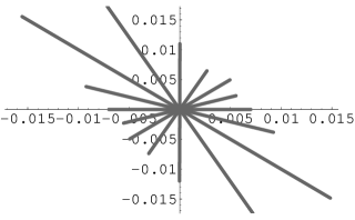
Figure 8: Initial velocity directions ${\bf v}(0)$ at $L_{4}$ whose magnitude corresponds to the associated critical breakout velocity $V^{*}(0)$, which are listed in Table LABEL:tab:1.

Note that the method, or algorithm, used above to estimate the critical velocities $V^{*}(0)$ at $L_{4}$ leading to breakout motion, is similar in nature to the method of estimating transitional stability regions, called weak stability boundaries, between capture and escape about the Moon described in Belbruno (2004). This capture region has important applications. It was used by one of us to find a new type of low energy route to the Moon in 1990 where lunar capture is automatic (Belbruno $\&$ Miller 1990). This special lunar transfer was designed in order to resurrect a Japanese lunar mission and enable the spacecraft Hiten to successfully reach the Moon in October 1991 with almost no fuel (Belbruno 1992; Frank 1994). More general references on this are (Adler 2000; Belbruno 2004; Belbruno $\&$ Miller 1993).

Other methods could be used to study the bifurcation from horseshoe to breakout motion such as the computation of suitable surfaces of section to the trajectories in phase space, and then monitoring the iterates of intersecting trajectories on the section. This would give a more complete knowledge of the phase space near breakout motion, but this approach is not necessary for our purposes. The algorithm we have described accurately determines when bifurcation occurs.

We have also performed an analysis to understand the relationship of the critical breakout velocities as a function of the mass of the Earth $m_{2}$. It is found that roughly

$$V^{*}(0)\propto m_{2}^{1/3}.$$

As an example, we consider the two cases: $m_{2}=.1m_{E},.01m_{E},\ \ m_{E}=.000003$. When $m_{2}=.1m_{E}$, then for $\alpha=0,\pi/2,\pi,3\pi/2$, we obtain $V^{*}(0)=.004,.007,.004,.007$, respectively, and for $m_{2}=.01m_{E}$, we obtain $V^{*}(0)=.002.,003,.002,.003$, respectively.  These results imply that $V^{*}(0)\sim 0.6m_{2}^{1/3}$ for $\alpha=0,\pi$, and when $\alpha=\pi/2,3\pi/2,\ \ V^{*}(0)\sim m_{2}^{1/3}$. (Thus a giant impactor trapped in a stable orbit about $L_{4}$ and unperturbed will remain trapped there as the proto-Earth grows by accretion. Breakout velocity increases as the proto-Earth grows, postponing breakout, but at late times after the proto-Earth has reached essentially its full mass, according to our scenario, perturbations can drive the giant impactor to breakout.)

This concludes the demonstration of R1.

Demonstration of R2

We first show how to readily find trajectories from $L_{4}$ which collide with the Earth. The value of $\alpha=\pi/2$ is again considered, and we consider the case $V(0)=.012\stackrel{{\scriptstyle>}}{{\sim}}V^{*}(0)$ shown in Figure 7. Plotting the distance $r_{2}$ between $P_{3}$ and the Earth for $t\in[0,1000]$ reveals the times of the various Earth fly-bys. It was found that the case of $V(0)=.012$, for the given range of $t$, had very close Earth fly-bys, but no actual collision. Randomly altering this value of $V(0)$ yielded a collision on our second random choice of values of $V(0)=.0119981$. This is seen by plotting $r_{2}$ as a function of time shown in Figure 9

Figure 9: Variation of distance $r_{2}$ of $P_{3}$ to $P_{2}$(earth) as a function of $t\in[0,1000]$ in dimensionless units, $V(0)=.0119981$.

By magnifying the regions near minima of $r_{2}$ it can be seen which ones may yield collision. In this case, counting from the left to the right, we determined that the first, fourth, fifth minima yield distant fly-bys at over 1 million km. Thus, in these cases, the Earth fly-bys are not of interest. The third fly-by misses the Earth by about 18,000 km. However, it is found that the second fly-by in fact collides with the Earth. The time of collision with the surface of the Earth is at $t=360.181558$, corresponding to 57.3247 years. This time is calculated when the center of the impactor, viewed as a circle of radius $r_{I}=3397$ km, intersects the surface boundary of the Earth, which is at a radial distance $r_{E}=6378.14$ km, from the Earth’s center. This is seen in Figure 10.

Figure 10: Distance $r_{2}$ of $P_{3}$ to $P_{2}$(earth) goes below the earth’s radius .0000426346(i.e. 6378.14 km) proving collision has occurred. $V(0)=.0119981$. Plot is $t$ vs $r_{2}$ in dimensionless units.

The horizontal line indicates the Earth’s radius of 6378.14 km here represented by the value $r_{2}=.0000426346$. The time of collision with the surface of the Earth is at $t=360.181558$, corresponding to 57.3247 years. We are assuming that each point of the trajectory of the impactor at any given time is at the center of the impactor. More accurately, however, collision actually occurs a few moments earlier when the surface boundary, circle, of the impactor touches the surface boundary, circle, of the Earth. That is, when $r_{2}=r_{I}+r_{E}=9775.14$ km, where for $r_{I}$ we take the radius of Mars, since this is a Mars-sized object, or, in dimensionless units, when $r_{2}=.00065342$. In general, we assume collisions mathematically occur in our numerical simulations when $r_{2}\leq.00065342$.

We now show what the collision trajectory looks like and discuss its properties. The collision trajectory, $Cl$, is shown in Figure 11.

Figure 11: Entire collision orbit (x vs y)- Originating at $L_{4}$ at $t=0$ and colliding with the earth when $t=360.18$ or, equivalently, $57.32$ years, $V(0)=.0119981$, Sun centered.

It starts at $L_{4}$, moves in a posigrade fashion toward the Earth, turns around and in a retrograde motion moves around the Sun to collide with the Earth. A view of this orbit in its final 9.57 years is shown in Figure 12.

Figure 12: Orbit approaching collision with the earth (x vs y). Time duration of 9.57 years shown, $t\in[300,360.181558]$, axis earth centered.

Collision with the Earth itself and the final 9.14 hours of the trajectory are shown in Figure 13.

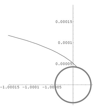
Figure 13: Collision of the impactor with the earth, x vs y. Final 9.14 hours of trajectory shown, earth centered.

In this figure we stopped the trajectory of the impactor before its Earth periapsis. However, if it were continued beyond collision it would reach its periapsis point approximately on the $x$-axis inside the Earth’s radius at $t=360.1817$ where $r_{2}=.00003$. (See Figure 14).

Figure 14: Continuation of collision orbit across the $x$-axis when $t=360.1816$, x vs y, earth centered.

If it were extended so that $t\in[0,1000]$, the trajectory would be as shown in Figure 15.

Figure 15: Extended collision orbit, through collision, $t\in[0,1000]$ ( i.e. $t\in[0,159.15]$ years), x vs y, Sun centered.

This figure for $V(0)=.0119981$ is shown to compare with Figure 7 for $V(0)=.012$ indicating the sensitive, or chaotic, nature of the breakout motion, where a difference of $V(0)$ by .000002 yields a qualitatively different appearing trajectory. The chaotic nature of the motion near breakout is also seen in Figure 16, which is a plot of $r_{2}$ for $V(0)=.0119986$, when compared to Figure 9 where $V(0)=.0119981$.

Figure 16: Variation of $r_{2},t\in[0,1000]$, for $V(0)=.0119986$. Compare with Figure 9, where $V(0)$ differs by .0000005.

It is seen that although the difference in $V(0)=.0000005$ at $L_{4}$, there is a significant difference in the qualitative appearance of the two plots. This is caused by the fact that infinitesimally small changes in $V(0)$ at $L_{4}$ can cause slightly different Earth fly-by conditions which over long time spans, $t\in[0,1000]$ can cause the trajectory to change noticeably if any of the fly-bys are close. However, as we will see in the following, close fly-bys will only yield negligible Kepler energy increases with respect to the Sun. So, although the trajectory may have a qualitative different appearance, it will still have approximately the same Kepler energy before and after close fly-bys. The change in the trajectories for tiny changes in $V(0)$ observed is typical for chaotic motion in general, and is a sign that a hyperbolic invariant set likely exists in the phase space for the breakout motion of $P_{3}$. A hyperbolic invariant set in general is a Cantor set all of whose points are have a saddle-like structure produced by a transverse homoclinic orbit, whose existence is given by the Smale-Birkhoff theorem (Belbruno 2004). The use of the term chaotic in a strict mathematical sense means the existence of a hyperbolic invariant set.

It is remarked that $Cl$ represents a physical collision with the surface of the Earth, where, at periapsis below the Earth’s surface, $r_{2}=.00003$. It turns out that actual pure collisions where $r_{2}\sim 0$ to high precision are readily found as well. For example, $V(0)=.011998$ leads to a pure collision at $t=360.1898$. In this type of collision, $P_{3}$ asymptotically approaches the collision manifold which is a set of measure zero.

It is observed that since the motion of $P_{3}$ repeatably passes near to the Earth in breakout motion, the Earth tends to readily pull $P_{3}$ toward pure and physical collisions. The set, or manifold, of pure collision trajectories are a subset of physical collision trajectories, and, in fact, are a set of measure zero in the four-dimensional phase space of position and velocity (Belbruno 2004). Since they are a set of measure zero, their near occurrence is reflective of the fact the fly-bys of the Earth are close and that the Earth has a considerable gravitational focusing effect when the trajectory is near parabolic.

It turns out that $Cl$ is approximately parabolic at collision. This is seen by plotting the Kepler energy $E_{2}$ of $Cl$ with respect to the Earth. In inertial Earth centered coordinates, ${\mathbb{X}}=(X_{1},X_{2})$, $E_{2}={1\over 2}|{\mathbb{\dot{X}}}|^{2}-{\mu\over{|{\mathbb{X}}|}}$. In barycentric rotating coordinates ${\bf x}=(x_{1},x_{2})\equiv(x,y)$, $E_{2}$ is transformed into

$$E_{2}={1\over 2}|{\mathbb{\dot{x}}}|^{2}-{\mu\over{r_{2}}}+{1\over 2}r_{2}^{2}-L,$$ (5)

where, $r_{2}=\sqrt{(x_{1}+1-\mu)^{2}+x_{2}^{2}},\ \ L=\dot{x_{1}}x_{2}-\dot{x_{2}}(x_{1}+1-\mu)$,   (Belbruno 2004, 2002). $L$ is the angular momentum of $P_{3}$. $E_{2}$, (5), is evaluated along $Cl$ and plotted in Figure 17 as a function of $t\in[0,360.181558]$. From Figure 18, $E_{2}=.000054$ at collision, which is nearly parabolic.

Figure 17: Kepler energy $E_{2}$ with respect to $P_{2}$ as a function of $t$ along entire collision orbit. It is seen that $E_{2}\rightarrow 0$.

Figure 18: $E_{2}$ as a function of $t$ at the end of the collision orbit approaching the value of .0000541 at periapsis below the earth’s surface, where $r_{2}=.00003$ (i.e. 4488 km), for $t=.00014$ (i.e. 12 minutes) beyond earth collision, $t\in[360.175,360.1817]$.

(If the collision were purely parabolic then $E_{2}=0$.) This yields a very slight hyperbolicity whose hyperbolic excess velocity with respect to the Earth, $V_{\infty}=\sqrt{2E_{2}}$, has the value of .0104. This is equal to $V^{*}(0)$ for $\alpha=\pi/2$ to within .0014. In scaled coordinates, $V_{\infty}=310m/s$ and $V^{*}(0)=328m/s$. $V_{\infty}$ is close to $V^{*}(0)$ because at Earth periapsis $V^{*}(0)$ is like the velocity at infinity. This velocity is approximately maintained along the orbit as it approaches collision. At actual Earth fly-by at periapsis the velocity with respect to the Earth increases due to the attraction of the Earth, and for this collision orbit $V=.44$ at Earth periapsis.

In (Belbruno $\&$ Gott 2004) it is analytically shown that in the critical or near critical breakout motion, all close Earth fly-bys, including collision trajectories, are approximately parabolic at periapsis. For critical breakout trajectories, which start at $L_{4}$ at time $t=0$, $V(0)=V^{*}(0)$. For near critical breakout motion we assume that $V(0)\stackrel{{\scriptstyle>}}{{\sim}}V^{*}(0)$. Notationally, $V(0)\stackrel{{\scriptstyle\geq}}{{\sim}}V^{*}(0)$ includes both of these cases.

We define the terms, ’close Earth fly-by’, ’approximately parabolic’. Let $\gamma(t)$ be a trajectory which performs a fly-by of the Earth, with a periapsis distance $r_{2}$ at some time $t$. We say that this is a close Earth fly-by if $r_{2}\leq 100,000$ km, or in dimensionless coordinates, $r_{2}\leq.000668$. The figure of 100,000 km is arbitrarily chosen since for weakly hyperbolic fly-bys of the Earth beyond this distance, the effect of an Earth gravity assist is negligible. Physical collisions are included as close fly-bys.

We use $E_{2}$ to determine the type of collision, which is computed at Earth periapsis. So, in the case of physical collision at the Earth’s surface, we propagate the trajectory to Earth periapsis within the Earth. This point occurs at a very short time after physical collision which for the case of $Cl$ is only 12 minutes. At the periapsis point $E_{2}$ is evaluated at the trajectory state of position and velocity. If $|E_{2}|\stackrel{{\scriptstyle>}}{{\sim}}0$, the collision or collision trajectory is called approximately parabolic. It could be slightly elliptic, slightly hyperbolic or purely parabolic. It turns out, as we will see, that for break out or near breakout motion, the fly-bys are all approximately parabolic. The following result is obtained (For details see Belbruno $\&$ Gott 2004):

For the set of critical or near critical breakout velocities at $L_{4}$, the value of $E_{2}$ at the close Earth fly-bys at periapsis has the value

$$E_{2}\approx{1\over 2}V(0)^{2}\stackrel{{\scriptstyle\geq}}{{\sim}}{1\over 2}V^{*}(0)^{2}\stackrel{{\scriptstyle>}}{{\sim}}0;$$ (6)

That is, the close Earth fly-bys are approximately parabolic. This is true for all the values of $\alpha$ except those values in small neighborhoods of $5.102\pi/8,13.5\pi/8$ (see comment below).

This implies that a trajectory $\gamma(t)$ starting near critical breakout velocity at $L_{4}$ for $t=t_{0}$ will satisfy equation 6 for any future time $t>t_{0}$ corresponding to any close Earth flyby at periapsis.

More precisely, as shown in Belbruno $\&$ Gott 2004, for a trajectory starting at $L_{4}$, at Earth periapsis on a close Earth fly-by at a distance $r_{2}=\delta_{2}$,

$$E_{2}={1\over 2}V^{2}(0)\ +\mathcal{O}_{0}(\mu)+\mathcal{O}_{1}(\delta_{1})+\mathcal{O}_{2}(\delta_{2})$$ (7)

where $\mathcal{O}_{0}=3\mu,\ \mathcal{O}_{1}=2\delta_{1},\ \mathcal{O}_{2}=2\delta_{2}\cos\theta_{2}$, $r_{2}=\delta_{2}<.000668\ll 1,\ r_{1}=1+\delta_{1},\ |\delta_{1}|<.000668,\ |\delta_{1}|\geq 0,\ \delta_{2}\geq 0.$ This relation yields (6) for $\mu,\delta_{1},\delta_{1}$ small.

Let $P_{3}$ be at $L_{4}$(or $L_{5}$) at $t=0$, and let ${\bf v}(0)$ be the initial velocity with magnitude $V(0)=|{\bf v}(0)|$. Then, the Jacobi integral $J$ has the value $J=C_{0}=3\ -V^{2}(0)\ -\mu(1-\mu)$. This implies that for the set of critical breakout velocities $V^{*}(0)$ at $L_{4}$ for $\alpha\in[0,2\pi]$ (see Figure 8), $C_{0}\stackrel{{\scriptstyle<}}{{\sim}}3$.

As mentioned earlier, there are two sharp spikes in the breakout velocities shown in Figure 8 of values .22, .25 which occur for $\alpha=5.102\pi/8,13.5\pi/8$, respectively. However, most values of $V^{*}(0)$ vary between approximately $.006$ and $.05$ if two intervals in $\alpha$ of total width approximately $.157$ radians are deleted near where the spikes occur. This implies that for nearly all of the values of $\alpha$, equation (6) implies that approximately

$$E_{2}\in[.000018,.0012].$$ (8)

Thus, $P_{3}$ is approximately parabolic at collision. The range given by (8) is a crude estimate of $E_{2}$. The observed value for $Cl$ of $E_{2}=.000054$ is contained within this interval. A sharper estimate can be made using (7). For $Cl$, $V(0)=.0119981$, and at fly-by periapsis, below the Earth’s surface, $r_{2}=\delta_{2}=.00003$. This occurs approximately on the $x_{1}-$axis implying $r_{1}=-\delta_{1}=-.00003,\ \theta_{2}=0$. Substitution of $V(0),r_{1},r_{2},\theta_{2}$ into (7) yields the value, $E_{2}\approx.00007$. Noting that the numerically observed value of $E_{2}$ at periapsis for $Cl$ $E_{2}=.000054$, the predicted value is in error by only .000016 demonstrating the accuracy of the predicted values.

We remark that in all the cases numerically observed, $E_{2}$ was not negative(i.e. the orbit was not elliptic) during the fly-by. Some such fly-bys are likely to exist due to the chaotic nature of breakout motion, however, the probability of finding trajectories with elliptic fly-by states is apparently small. Their chaotic structure and low probability of occurrence is studied in Belbruno (2004). When $E_{2}$ is near to zero this defines weak capture studied in Belbruno (2004), where $P_{3}$ will, in general, move about the Earth in a chaotic fashion generally leading to escape or collision. However, as remarked, the case of interest here is when $E_{2}$ is very slightly hyperbolic.

The retrograde collision trajectory $Cl$ emanating from $L_{4}$ is paired with another symmetric collision trajectory $Cl^{*}$ emanating from $L_{5}$ which is symmetrical to $Cl$ and moves in a posigrade fashion about the Sun. This follows by the symmetry of solutions mentioned in Section 2. It will collide with the Earth in the 4th quadrant as shown in Figure 13.

Probability of Collision at Breakout for the Restricted Problem

A measure of the likelihood of finding collision trajectories is now described. This is done for the four basic initial velocity directions at $L_{4}$: $\alpha=0,\pi/2,\pi,3\pi/2$. For an initial velocity of $P_{3}$ at $L_{4}$ for a given $\alpha$ we assume the corresponding breakout velocity $V^{*}(0)$ as shown in Figure 8. The orbit of $P_{3}$ is propagated from $L_{4}$ for $t\geq 0$ and since it is in breakout motion we know that it will not be in horseshoe motion, but will cycle about the Sun and repeatably fly past the Earth. We can numerically demonstrate that collision with the Earth is likely. This intuitively makes sense since the fly-bys will be close and the the annular region supporting the breakout motion is narrow. Now, for a given initial velocity at $L_{4}$ for $t=0$ we see from Figure 8 that $V^{*}(0)$ is given up to three digits. For a given value of $V^{*}(0)$, depending on $\alpha$, we propagate the trajectory for up to $t=4000$, which corresponds to 637 years, and see if collision has occurred. $t=4000$ is chosen arbitrarily, for convenience and is fairly small in astronomical terms. If no collision occurred in that time, then we give $V^{*}(0)$ a random perturbation by adding to it the random number $.000mn$, where $m,n$ are positive random integers ranging from 0 to 9. For a choice of $m,n$ the trajectory is propagated again. If collision does not occur, we repeat the process again for a different choice of $m,n$, continuing trials until success is achieved.

For $\alpha=0,\pi/2$, we required two random trials for success, where success means we achieve collision within $t=4000=637$years. For $\alpha=\pi$, three random trials were required until we have success, and for $\alpha=3\pi/2$, six random trials were required for success. Therefore we have achieved success in four random trials out of thirteen. This gives our best estimate of the probability $\mathcal{P}$ of success for $0\leq t\leq 4000$ as

$$\mathcal{P}\sim{4\over 13}.$$ (9)

If we had not limited ourselves to $t=4000$ the probability would have been larger. This probability is discussed in further detail in the Appendix. We have run a sufficient number of trials to produce a rough order of magnitude estimate of this probability which is sufficient for our purposes, but a large number of additional trials could establish this number to higher accuracy.

It is noted that the gravitational focusing on $P_{3}$ to cause a collision is substantial. This is related to the fact the breakout motion is occurring at a fixed energy for the planar restricted problem. The fixed energy yields a three-dimensional energy surface obtained from the Jacobi integral. As is proven in Belbruno (2004), the manifolds leading to collision at $P_{2}$ are two-dimensional, and although they are a set of measure zero, the particle $P_{3}$ is readily able to move asymptotically close to these surfaces and to collision after the gravitational focusing. The collision manifolds on the Jacobi integral surface separate the phase space, so it is fairly easy for $P_{3}$ to get near to the collision manifold. In higher dimensions this separation of the phase space on the Jacobi surface does not occur, and the collision manifold is more elusive.

This concludes the demonstration of R2.

It is interesting that these creeping chaotic orbits seem to lead naturally to collision with Earth (as proposed by the giant impactor theory) rather than to capture into a bound orbit (as in the sister planet theory). If one wanted to have a sister planet theory, of course, $L_{4}$ would be a promising place for the Moon to start out. So it is significant that our chaotic creeping orbits (slightly hyperbolic-nearly parabolic) lead naturally to collision rather than capture. This favors the giant impactor theory. The sister planet theory would of course also have a problem with the difference in iron between the Earth and the Moon.

Random Walk, $\Delta V$ Accumulation, and Relevant $V(0)$ Range

In determining $V^{*}(0)$ at $L_{4}$ above, we kept $P_{3}$ fixed at $L_{4}$ and gradually increased $V(0)$ for a given velocity direction. This yields a well defined set of $V^{*}(0)(\alpha)$ for $\alpha\in[0,2\pi]$.

We now consider a more realistic way that $P_{3}$ would increase its velocity in a gradual fashion. The mechanism for this is to assume that $P_{3}$ is randomly being perturbed by encountering other planetesimals(whether by gravitational encounter or direct collision) and in each encounter, it acquires an instantaneous kick $\Delta V$. So, it is not kept fixed at $L_{4}$. To make this more realistic, we assume that the times of encounters are random, within a large range, and the direction $\alpha$ of the kicks are random. The only thing we normalize is the magnitude of the $|\Delta V|$’s which for convenience is held fixed.

Thus, $P_{3}$ starts at $L_{4}$ with a zero velocity, and at time $t=t_{1}=0$ a velocity $V(0)=\Delta V$, is applied in a random direction. This yields a vector ${\mathbb{v}_{1}}$ with magnitude $\Delta V$. $P_{3}$ moves on a trajectory $\gamma(t)$ in a neighborhood of $L_{4}$, assuming that the value of $\Delta V$ is small. At a random time $t_{2}>0$ another velocity vector ${\mathbb{v}}_{2}$ of random direction and magnitude $\Delta V$ is vectorially added to $P_{3}$’s velocity at $t=t_{2}$. Then the trajectory is propagated for $t>t_{2}$ until at another random time $t_{3}>t_{2}$ a random vector ${\mathbb{v}_{2}}$ of magnitude is vectorially added to $P_{3}$’s velocity vector at $t=t_{3}$, and this process continues creating a sequence $t_{k}$ of times, $t_{k+1}>t_{k}$, and velocities ${\mathbb{v}}_{k},k=1,2,3,\ldots.$

While the $\Delta V$’s are being applied, the trajectory $\gamma(t)$ is gradually moving further from $L_{4}$, but since the velocity directions ${\mathbb{v}_{k}}$ are applied randomly, the path of the trajectory $\gamma(t)$ will move further away from $L_{4}$ for some time spans, and then move toward $L_{4}$ for others. However, as $k$ increases, one would expect, by the principle of random walk, for $P_{3}$ to eventually escape $L_{4}$ and creep toward the Earth for $k$ sufficiently large when the velocities ${\mathbb{v}}_{k},k=1,2,3,\ldots$ applied on the trajectory $\gamma(t_{k})$, gradually accumulate to a sufficiently large magnitude for breakout to occur. If the ${\mathbb{v}}_{k}$ were all applied in the direction of motion of $P_{3}$ at $t_{k}$, then the magnitudes $\Delta V$ would add producing an cumulative velocity addition of $k\Delta V$ at the $k$th step. However, the directions of ${\mathbb{v}}_{k}$ are random, and by the principle of a random walk, the number of encounters $k$ before ejection occurs should be expected to instead satisfy

$$\sqrt{k}\Delta V\approx.006$$ (10)

for $k$ sufficiently large(and $\Delta V$ sufficiently small) where $.006$ is approximately the minimum value .0057 of $\{V^{*}(0)\}$. This makes dynamical sense, since as the $\Delta V$’s are applied, the trajectory $\gamma(t)$ would seek to minimize the Jacobi energy, and hence the velocity, along its path. We found in all our numerical simulations the following result:

For a given value of $\Delta V$, the number $k$ of random ${\bf v}_{k}$ applications required for breakout to occur approximately satisfies (10).

We describe this process of random walk $\Delta V$ accumulation, and its verification.

For convenience we choose $\Delta V=.001$ and start at $L_{4}$ with zero initial velocity. (10) implies that $k$ should satisfy $\sqrt{k}\Delta V\sim.006$, which yields $k\cong 36$. It was found that breakout occurred when $k=36$ as predicted. Random kicks of velocity $\Delta V$ were applied in random directions $\alpha_{k}$ and after random time intervals $t_{k}$. (As in all future runs the times between kicks are just chosen to be large enough to randomize the position. The real time for random walkout is expected to be much longer in years - perhaps 30 million years as considered in the Appendix.)

From the above, we have the following result,

(Random Walk $\Delta V$ Accumulation)   Under a realistic assumption of random walk, the peculiar velocity for $P_{3}$ accumulates proportional to the square root of the number of encounters until it reaches a breakout state. Since a random walk is isotropic the peculiar velocity is likely to encounter the breakout state first at a point near the minimum value of .006 of the set $\{V^{*}(0)\}$ thus giving (10).

Therefore, substituting $V^{*}(0)=.006$ into (6) implies that for close Earth fly-bys resulting from the random walk process at or near breakout, $E_{2}\approx.000018$. This implies that at close Earth fly-by resulting from the random walk process, a nominal value of $V_{\infty}=.006$ which is 179 m/s. When $P_{3}$ does a close fly-by of the Earth, after passage through periapsis it will receive a gravity assist and increase, or decrease, its velocity with respect to the Sun. A measure of this velocity change is observed due to the bending of the trajectory of $P_{3}$ as it passes through periapsis. For example, this bending is clearly seen in Figure 14. The more distant the fly-by, then in general the less the bending. The maximum bending is obtained from pure collision trajectories, where the bending angle is $\pm\pi$. It is determined in Broucke (1994) that the resulting change in magnitude of the velocity, $\delta v$ with respect to the Sun due to gravity assist is maximally, $2V_{\infty}$. Thus, for each close Earth fly-by, the expected maximum gain in velocity magnitude is approximately 358 m/s. In general, they will be less.

The maximal velocity of 358 m/s is a relatively small number and will have little effect on a breakout trajectory when it has a close Earth fly-by. This velocity is less than .012 of the orbital velocity, inducing eccentricities into the trajectory of $P_{3}$ after fly-bys of at most this order. It is found in general that within time spans on the order of 2000 time units, there are generally only one or two close Earth fly-bys. This implies that $P_{3}$ will remain in breakout motion about the Sun in a relatively thin annular region for very long periods of time, generally tens of thousands of time units, and repeatably pass by the Earth without being ejected.

Collisions in Three Dimensions and the Mars Sized Impactor

Thus far we have constrained $P_{3}$ to lie in the plane of motion of the Earth and Sun in the planar restricted three-body problem. It that situation it was seen that collision trajectories are readily found. When the motion of $P_{3}$ has an out of plane component, $z$, added to it, it is more complicated. In this case we have the three-dimensional circular restricted three-body problem, defined exactly the same way as for the planar problem, except that $P_{3}$ can move in the $z$ direction, see (Szebehely 69; Belbruno 2004). By continuity with respect to initial conditions, it must be the case that collisions in the planar case will persist in the three-dimensional case if $|\dot{z}|$ is sufficiently small. A way to approximately get a measure of the maximal allowed $z$ motion is to consider a collision trajectory from $L_{4}$ to the Earth generated at or near critical breakout, and then see how much $\dot{z}$ can be added at $L_{4}$ and still maintain collision with the Earth which is now a three-dimensional sphere. This is a relatively straight forward calculation.

In the Appendix we show that Earth collisions should persist providing $|\dot{z}|\stackrel{{\scriptstyle<}}{{\sim}}.0034$. This implies a thin disk of planetesimals. In the Appendix we show that a disk of thickness $28r_{E}$ easily satisfies this requirement. This has an angular width of 4.1 minutes of arc as seen from the Sun. Although this seems thin, it turns out that inner B, A rings of Saturn, extending from 92,000 km to 140,210 km, have a thickness of .18 - 1.7 seconds of arc as seen from the center of Saturn, which is even thinner than required in our situation.

The modeling of most interest in this paper is for the general three-dimensional three-body problem defined by equation 4, where $m_{3}=.1m_{2}\neq 0$, so a Mars-sized Earth impactor is modeled. This is used by Canup $\&$ Asphaug (2001). Although the motion of the Earth, $P_{2}$, is given initial conditions for uniform circular motion, about the Sun, $P_{1}$, it need not remain circular as time progresses due to the gravitational perturbations of $P_{3}$. This property makes the problem more interesting. To better understand this and to see its effect on collision trajectories, the general planar three-body problem is first considered. It is defined from (4) by setting $X_{k3}=0,k=1,2,3$.

As with the restricted problem, a rotating coordinate system $(x,y)$ is chosen, this time, rotating with the mean motion of the Earth about the Sun. In this system the Earth is not fixed on the -$x$ axis as in the restricted problem since it is perturbed by $P_{3}$ especially during fly-bys.

Just as in the restricted three-body problem, breakout from $L_{4}$ can be defined for the general planar three-body problem with exactly the same methodology as for the restricted problem, by gradually increasing the velocity of $P_{3}$ at $L_{4}$ until breakout is achieved, for any given velocity direction. Nearly identical results are obtained as in R1(Figure 8) and this analysis is not duplicated for this situation. The desired random walk $\Delta V$ accumulation process is defined exactly as before for this current problem, and we have verified that the same results are obtained.

We determine the breakout of $P_{3}$ to Earth collision as we did in the restricted problem by gradually increasing the velocity at $L_{4}$ until a critical velocity is reached. That is, we are not modeling the random walk process, and are copying the procedure we performed for the restricted problem. This is done to keep the modeling as close as possible to the restricted problem in order to better understand how $P_{3}$ perturbs $P_{2}$ and the effect this has on obtaining collision trajectories.

An important difference in using the planar three-body problem instead of the restricted problem is observed when the breakout velocity is determined for $P_{3}$ at $L_{4}$. As the velocity magnitude $V(0)$ for $t=0$ is gradually increased at $L_{4}$, and $P_{3}$ moves in the horseshoe regions about the Sun, the location of the Earth moves in its orbit, approximately maintaining its 1 A.U. distance from the Sun, but shifting its angular position with respect to the Sun. This is because as $P_{3}$ creeps further and further away from $L_{4}$ approximately on Earth’s orbit, it can gravitationally perturb the Earth when it moves relatively near to the Earth since its mass is now one tenth that of Earth. Analogous to the restricted problem, when $V(0)$ gets close to the breakout value, the horseshoe region begins to close on itself in a symmetrical way with respect to the Earth. However, since the Earth has shifted its location, the symmetrical closing point is not on the $x$-axis as in Figure 5 for the restricted problem, but at another location, the Earth’s location, approximately 1AU from the Sun. This is illustrated in Figure 19 where $V(0)\equiv|(\dot{x},\dot{y})|=.160$ km/s. $\alpha=0$ is assumed. This is fairly close to breakout, for the given velocity direction, which occurs for $V(0)=.205$ km/s. The final location of the Earth when breakout is achieved is in the third quadrant about 20 degrees from the $-y$-axis which means that the $x$-axis is not fixed to the Earth but to the mean motion.

Figure 19: $\gamma(t),V(0)=.160$ km/s, $t\in[0,200]years$, x vs y, Sun centered.

The cases we have examined indicate that the likelihood for collision to occur in this problem is similar to that of the restricted problem. However, the dynamics of collision is more complicated.

We now examine a collision trajectory, $Cl2$ and the associated dynamics. $Cl2$ occurs in the breakout state for $V(0)=205$ km/s. This is only discussed briefly here as the details can be found in Belbruno $\&$ Gott (2004). It starts at $L_{4}$ for $t=0$ with a velocity of .205 km/s in the positive $x$-direction. The Earth is located initially on the negative $x$-axis at 1AU distance from the Sun, at the origin.

$Cl2$ is plotted in Figure 20

Figure 20: $CL2$ from $L_{4}$ at $t=0$ to earth collision at t = 108.628235 years in the third quadrant. Sun centered, x vs y.

In Figure 20 in the rotating coordinate system $P3$ escapes $L_{4}$ moves down toward the Earth, then turns around and moves in a retrograde motion (clockwise) about the Sun, continuing to the third quadrant, and then in a posigrade motion (counterclockwise) with respect to the Sun, it circles the Sun, moves past the negative $x$-axis, to Earth collision. Unlike $Cl\equiv Cl1$, $Cl2$ is a posigrade collision orbit.

Now, as $P_{3}$ has moved in this collision orbit, the Earth has moved also. It has moved in the posigrade direction and then, toward the end in a complicated motion in the retrograde direction. This is seen in Figure 21

Figure 21: The motion of the earth from $t=0$ to collision with $P_{3}$ on $Cl2$ at t = 108.628235 years, x vs y.

The motion of the Earth about 30 years prior to collision with $P_{3}$ is complicated. The final phase of the Earth’s motion much enlarged is shown in Figure 22. It consists of many small loops, one for each year, caused by the perturbation of $P_{3}$ as it gets near to collision. In Figure 22, this looping motion is shown in large scale about four years prior to collision with $P_{3}$. The Earth is moving in a retrograde fashion in this figure, starting in the lower right and ending in collision near the center of the coordinate system. The very end of the Earth’s trajectory is actually parabolic in appearance, as seen in Figure 24, which is too small to be seen in Figure 22.

Figure 22: The motion of the earth(note enlarged scale) about 4 years prior collision with $P_{3}$ on $Cl2$ at t = 108.628235years. x vs y.

In the same time frame as in Figure 22, we show $P_{3}$ on $Cl2$ moving to collision with the Earth in Figure 23. The small black smudge on the lower left is the complicated motion of $P_{2}$(shown enlarged in Figure 22) prior to collision which relative to the scale of $Cl2$ is too small to be clearly seen.

Figure 23: $Cl2$ 4 years prior collision with the earth at t = 108.628235years. x vs y.

The actual Earth collision with $P_{3}$ is shown in Figure 24 which shows the relative motions of the Earth and $P_{3}$. We have integrated the motion of $P_{3}$ through collision to better show the relative motions. In this figure, $Cl2$ is the larger parabolic type curve, and the Earth moves in the smaller curve. The Earth moves clockwise from the left to the right, and $P_{3}$ moves clockwise from the right to the left. The span of the vertical axis is approximately 20000 km, so that one half of this distance represents the radii of the Earth and $P_{3}$ added together. This implies that actual physical collision between the Earth and $P_{3}$ occurs in this figure when $P_{3}$ is near the start of its motion on the bottom right. We have verified that this is a near parabolic collision as in $Cl1$.

Figure 24: Relative motions of the earth and $P_{3}$ near collision. $CL2$ moves on the larger parabolic curve clockwise from right to left, and the earth moves on the smaller parabolic curve clockwise from left to right. Time Duration: 1.9 hours. x vs y.

Three-Dimensional Simulation of Collision in an Anisotropic Thin Planetesimal Disk via Random Walk Encounter Dynamics

We now consider the main model of this paper for the numerical simulation of a collision trajectory by a Mars-sized impactor. So, the planar three-body problem just considered is now generalized to three-dimensions given by (4). At $t=0$ the Earth has the same initial position position as in the planar case, and $P_{3}$ starts at $L_{4}$. We now more realistically model the breakout of $P_{3}$ from $L_{4}$ by the random walk $\Delta V$ accumulation process.

We assume that $\Delta V$’s are imparted to $P_{3}$ at random times. We will also assume that at these random times separate independent $\Delta V$’s are imparted to the Earth. As is described in the Appendix, we are assuming a thin planetesimal disk, and at the random times, two types of velocity kicks are applied to both the Earth and $P_{3}$. One velocity kick is assumed to be in a random direction in the plane, and labeled $\delta V_{\|}$, and the other is perpendicular to the plane randomly either up or down and labeled $\delta V_{\perp}$. The velocity kicks applied to the Earth have a subscript of E, and those relative to $P_{3}$ have no subscript. In the Appendix we estimate the magnitudes of these velocities. The magnitudes for the velocity kicks for $P_{3}$ are given by (16) in the Appendix, and the magnitudes for the Earth are given by (18) in the Appendix. In this case breakout occurs when $k=14$. After these directions are input, the trajectory is propagated for a random time $t$ which varies between 0 and 100 years. The process is then repeated.

Once the breakout state was achieved in the 14th step, and the propagation terminated after $t_{14}=93.1$ years, it was found that by extending it another 6.9 years to 100 years, no collision occurred. We then went back to the beginning of the 14th step. A different set of random values were given to the velocity kick directions for both the Earth and $P_{3}$, keeping the time of integration to be from 0 to 100 years. Collision again did not occur. We then again went back to the beginning of the 14th step, and again picked random values, and collision also did not occur. We then made a third additional random trial for the velocity kick directions at the beginning of the 14th step and found collision did occur when $t_{14}\sim 4.56$ years.

This yields a probability of collision $\mathcal{P}=1/4$(because in one of four random trials we succeeded) we discuss this further in the Appendix. (As in the discussion following equation 9, our number of trials is sufficient to give a rough estimate of this probability which is all we require, and additional trials could establish this number to higher accuracy.)

The collision trajectory $\gamma(t)$ is plotted in Figure 25 from the initial value in the breakout state at the 14th step using the randomly chosen velocity kick directions in the final attempt. The time from its initial condition is 4.5615948 years, and this final portion of the trajectory $\gamma(t)$ is shown. In Figure 25 it is the upper curve, and the motion is in the downward direction. The smaller lower curve shows the motion of the Earth which moves in the upward direction. The collision is seen to take place near the $x-$axis(when the center of $P_{3}$ hits the Earth’s surface). Actual physical collision occurs slightly earlier when the surface of the impactor hit the surface of the Earth. If we continue the trajectory $\gamma(t)$ through the Earth’s surface to Earth periapsis, the periapsis distance is only approximately 200 km. The time of periapsis is 4.5616056 years. See Belbruno $\&$ Gott(2004) for more details.

The initial conditions for the Earth and $P_{3}$ at the beginning of breakout, 4.5615948 years prior to Earth collision are explicitly given in [5]. This breakout state results from the random walk process previously described after 13 velocity kicks at times $t_{i},i=1,2,...,13$, where $t_{14}=4.5615948$ years. The total time $T$ for the motion of $P_{3}$ to reach this state is $T=\Sigma^{14}_{i=1}t_{i}=728.2$ years. The position of the Earth at breakout shows that the Earth has migrated in its orbit a considerable distance in a posigrade fashion from its initial position on the negative x-axis to the first (upper right) quadrant approximately along its orbit. The velocity of the Earth has slightly changed to 29.773 km/s from 29.78 km/s due to perturbations of $P_{3}$. Even though collision with the Earth is 4.56 years away, the velocity of $P_{3}$ is 29.698 km/s which differs from that of the Earth by only 75 m/s.

We describe the collision trajectory of $P_{3}$ with the Earth. The coordinate system is the same that we used in describing the motion of $Cl2$; that is, a rotating coordinate system rotating with the mean motion of the Earth about the Sun. It is convenient use Jacobi coordinates ${\bf q}=(q_{x},q_{y},q_{z})\ \ {\bf Q}=(Q_{x},Q_{y},Q_{z})$, where ${\bf q}$ is the relative vector of the Earth with respect to the Sun, and ${\bf Q}$ is the vector from the center of mass of the binary pair $P_{1},P_{2}$ to $P_{3}$ (Belbruno 2004). As with the planar three-body problem we considered, we use a rotating coordinate system which initially rotates in the plane of the Earth about the Sun, and with the mean motion of the Earth about the Sun.

Figure 25: Collision between Earth(Lower curve) and Impactor(upper curve) in the first quadrant. Earth moves in upward (posigrade) direction, Impactor moves in downward (retrograde) direction. Collision occurs slightly above the x-axis. Time Duration: 4.5615948 years. Planar Projection, x vs y.

Along the collision trajectory $\gamma(t)$ of $P_{3}$ the $z$-variation between the Earth and $P_{3}$, given by $q_{z}-Q_{z}$, oscillates between approximately $\pm 2000$ km. This is shown in Figure 26.

Figure 26: Variation of $q_{z}-Q_{z}$. Time Duration: 4.5615948 years.

We show the relative motion of the Earth and $P_{3}$ near collision in Figure 27. In this figure the time duration is only .53 hours. The orbits of the Earth and $P_{3}$ have been continued beyond collision to get a better understanding of the dynamics. The vertical axis spans approximately 10000 km, so that actual collision of the surface of the impactor with the surface of the Earth would occur near the beginning of the trajectory $\gamma(t)$ in the upper right quadrant. This dynamics is analogous to that of $Cl2$ near collision shown in Figure 24.

Figure 27: Relative motions of the Earth(smaller parabolic curve) and Impactor(larger parabolic curve) near collision. Earth moves counterclockwise from left to right, Impactor moves counterclockwise from right to left. Time Duration: .53 hours. Planar Projection, x vs y.

As a final comment, it has been verified that including full solar system modeling, as described at the end of Section 2, the process of obtaining the collision trajectory $\gamma(t)$ is perturbed by a negligible amount, and a nearby collision trajectory can be constructed. This is due to the fact that at breakout, the motion of $P_{3}$ stays close to 1AU radial distance from the Sun. It is also noted that in our analysis of the motion of $P_{3}$ after breakout, it performs several close flybys of the Earth for several hundred years. During this time collision is fairly likely to occur. Our analysis has shown that it is most likely to occur soon after breakout, which for the trajectory $\gamma(t)$ was only 4.6 years. It has been found that after breakout has occurred $P_{3}$ generally makes very close flybys of the Earth for up to approximately 500 years, and then the flyby distance becomes steadily larger. The repetitive flybys increase the semi-major axis and eccentricity of the trajectory making collision less likely as $P_{3}$ is no longer restricted to staying as close to 1AU radial distance from the Sun as it did immediately after breakout. Also, $P_{3}$ will acquire larger deviations in the out of plane directions. Soon after breakout, these effects are significantly less pronounced. In this sense, soon after breakout $P_{3}$ has a good chance to creep into an Earth collision; however, if it does not have one relatively soon then the flybys themselves will eventually make collision less likely. Overall, as we have shown, the probability of collision with Earth rather promptly after breakout is appreciable (of order 1/4). As discussed previously, running additional cases could establish this number to greater precision.

4 Discussion

We have shown that the giant impactor could have formed at $L_{4}$($L_{5}$) and then escaped on a creeping chaotic trajectory to impact the Earth, with a near parabolic encounter in agreement with simulations.

We note that there are difficulties if the giant impactor came from a location other than $L_{4}$(or $L_{5}$). To illustrate this assume that it came from elsewhere.

Since the Earth’s orbit and Venus’ are nearly circular and co-planar even at the current epoch, after 4.5 billion years of perturbations, this suggests that the early disk of planetesimals in the neighborhood of the Earth was quite thin and that the planetesimals in the disk were in orbits that had low eccentricity (e) and inclination (i), $e\sim i\ll 1$. The critical impact parameter for collision with the Earth for a small planetesimal is

$$b_{m}=r_{E}(1+[V_{es}^{2}/V_{pec}^{2}])^{1/2},$$

where $V_{pec}$ is the peculiar velocity of the planetesimal, i.e., $V_{pec}\sim e\times V_{orb}\sim e\times 30$ km s^-1, and $V_{es}$ is the escape velocity from the surface of the Earth (see Appendix). If $V_{pec}/V_{orb}<0.004$, then $b_{m}\sim r_{E}(V_{es}/V_{pec})>e\times 1AU\sim i\times 1AU\sim(V_{pec}/V_{orb})1AU$, and the planetesimals whose semi-major axes are within a distance of $b_{m}$ of the Earth’s distance from the Sun of 1AU will likely suffer collision with the Earth within a short number of years since we expect the orbits to be chaotic, and the impact parameter with the Earth is less than the critical impact parameter $b_{m}$ for collision with the Earth. This will clear out a region of $\pm b_{m}$ around 1AU Except for planetesimals in stable orbits around $L_{4}$(or$L_{5}$). Planetesimals at nearly 1AU from the Sun–and not at $L_{4}$(or$L_{5}$)–will quickly be accreted by the Earth, before having the chance to grow large by accretion themselves. T.R. Cowley (lecture at Univ. of Michigan 2002) has noted this problem, saying that ”Advocates of the Big Whack hypothesis usually say that the impactor must have been formed near the Earth. This is neither probable nor impossible. It is not probable because the Earth could have readily swept up materials that would have formed the other body. It is not impossible because we do not know the precise conditions of the accumulation of the Earth, and cannot say how improbable assembly of the putative impactor near one astronomical unit really was.”) The stable location at $L_{4}$(or $L_{5}$) answers the probability question, offering a reasonably likely scenario for forming the giant impactor near 1AU without the material first being swept up by the Earth. Once this cleared out region of $\pm b_{m}$ has been established, there will be no further quick accretion onto the Earth, because the planetesimal’s orbits will not take them to within an impact distance $b_{m}$ from the Earth. Then they will have to diffuse in by two-body relaxation-from perturbations by other planetesimals and planets. This two-body relaxation process will slowly put planetesimals into the gap region again and there will be be quick accretion from the gap. The giant impactor is expected to be one of the later impactors to hit the Earth because the successful simulations of the formation of the Moon start with the Earth already at nearly its current mass, showing that its subsequent accretion (after the giant impactor hit) is assumed to be small (Canup $\&$ Asphaug 2001). The giant impactor should also be expected to be one of the latter impacts because planetesimals, including the Earth, grow by accretion with time and that would have also allowed more time for the giant impactor to have grown by accretion itself.

If the giant impactor is one of the latter impactors as argued by Canup $\&$ Asphaug (2001) (after most accretion for the Earth has been completed) then if it is not from $L_{4}$(or $L_{5}$) it must originally come from either significantly outside 1AU or significantly inside 1AU. But then it would violate one of the key advantages of the great impactor theory: namely, point (3) in the Introduction, which explains why the Earth and Moon have the same oxygen isotope abundance- namely that the Earth and the giant impactor came from the same radius in the solar nebula. Meteorites from different neighborhoods in the solar nebula(those associated with parent bodies of Mars and Vesta for example) have different oxygen isotope abundances. The impactor theory is able to explain the otherwise paradoxical similarity between the oxygen isotope abundance in the Earth and the Moon combined with the difference in iron.

The Earth has oxygen isotope abundances that are an average over all the planetesimals it has accreted–some initially from inside 1AU and some from outside. A giant impactor forming outside 1AU and drawn in by two-body interactions would have oxygen isotope abundances intermediate between Earth and Mars and therefore not identical with the Earth. Standard giant impact theory has the Moon formed primarily out of mantle material from the giant impactor material (see (Canup 2004)). The rest of the material in the giant impactor is absorbed by the Earth and the iron core of the giant impactor eventually finds its way into the Earth’s core, leaving the Moon iron depleted relative to the Earth. The Moon has been found to have a small core and this is assumed to be from giant impactor material. (See (Wänke 1999) for a discussion of how the giant impactor theory can accommodate this.) If the Moon derives from giant impactor material then it would have, the theory proposes, isotopic abundances identical with the Earth if it was formed near 1AU and this is observed to be the case (Clayton $\&$ Mayeda 1996; Wiechert et al 2001; Wänke 1999; Lodders $\&$ Fegley 1997 . But if the giant impactor came from significantly outside outside 1AU its isotopic abundances would be significantly different from that of proto-Earth. Furthermore, since $M_{I}$ is only 10$\%$ the mass of the Earth, this would pollute the proto-Earth’s isotopic abundances with only a 10$\%$ contribution from the giant impactor. This would give the Earth and the Moon different isotopic abundances, if the giant impactor came from significantly outside 1AU. A similar trouble occurs if the giant impactor originated significantly inside 1AU, if the oxygen isotope abundances inside 1AU are heterogeneous as well. (At present we have no meteorites in our possession whose parent bodies are thought to be Mercury or Venus. So we currently have no data for oxygen abundances inside 1AU.)

On the other hand, consider what happens if the giant impactor originated at $L_{4}$(or $L_{5}$). It is in a stable orbit, so it is not immediately accreted onto the Earth, and can grow large and hit the Earth later, alleviating the problem mentioned by Cowley. It sits nicely at 1AU and accretes exactly the same type of material the Earth does, some diffusing from outside 1AU, and some from inside. The integral of the oxygen isotope abundances of the accretion should be identical with that of the Earth. Eventually, perturbations kick the giant impactor out of its stable orbit and it collides quickly with the Earth. When the giant impactor hits the Earth and kicks out the Moon, since the Earth and giant impactor have identical isotope ratios, the Earth and Moon should have identical isotope abundances even though the Earth and Moon are polluted to different extents by giant impactor material. This is an advantage to the giant impactor model, producing automatic agreement with proposition (3) of the giant impactor model. Since this is one of the latter accretion events for the Earth in terms of the accumulation of its mass, the oxygen isotope abundances for the Earth and Moon will not be further significantly changed by post-giant impactor accretion.

Thus we propose the following scenario.

Debris remains at $L_{4}$ (as the Trojan asteroids prove). From this debris a giant impactor starts to grow like the Earth through accretion as described above. As the forming giant impactor reaches a sufficient mass ($\sim.1m_{Earth}$), it gradually moves away from $L_{4}$ through gravitational encounters with other remaining planetesimals and it randomly walks in peculiar velocity. It gradually moves farther and farther from $L_{4}$ approximately on the Earth’s orbit in a horseshoe orbit at 1AU, until it acquires a peculiar velocity of approximately 180 m/s. The giant impactor then performs breakout motion where it performs a number of cycles about the Sun, repeatably passing near to the Earth. In a time span roughly on the order of 100 years it collides with the Earth on a near parabolic orbit.

We present here a mechanism for the origin of a Mars-sized Earth impactor and describe the path it would take to arrive at Earth collision via a special class of slowly moving chaotic collision trajectories. The analysis shows that Earth collision along these trajectories is likely. Approaches for further work are discussed in the Appendix.

Note added in proof

As we have discussed, the giant impactor could have grown up in a stable orbit at Earth’s $L_{4}$ (or $L_{5}$) point where a stable orbit is possible and an object could remain and be able to grow by accretion without hitting the Earth early-on. We expect this phenomenon could occur when there was a thin disk of planetesimals (in nearly circular orbits). We have noted that Saturn’s rings are an example of such a thin disk of planetesimals(in this case, chunks of ice plus some dirt) observable today. Saturn’s regular icy moons (inside the orbit of Titan) are all in nearly circular orbits of low eccentricity suggesting that they formed out of a thin disk of planetsimals(ice chunks) rather like Saturn’s rings today only larger in extent. In such a situation we might expect our scenario to operate. Therefore it is quite interesting that we can find examples of objects at $L_{4}$ (or $L_{5}$), or escaping from $L_{4}$ (or $L_{5}$) in the Saturn system. Saturn’s moon Helene co-orbits at the $L_{5}$ point (60^o ahead) of the larger moon Dione. Helene has a largest diameter of 36 km and Dione has a diameter of 1120 km. Saturn’s moons Telesto (diameter 34 km) and Calypso (diameter 34 km) occupy both the $L_{4}$ and $L_{5}$ points relative to Saturn’s moon Tethys (diameter 1060 km). We would say that Helene, Telesto and Calypso originated in a planetesimal disk(of ice chunks) at these stable Lagrange points and have grown in place there surviving till the present without colliding with Dione or Tethys. The rest of the planetesimals(ice chunks) have accreted onto the regular moons of Saturn.(Saturn’s rings themselves lie inside the Roche limit where the formation of large objects is forbidden by accretion.) While these Lagrange moons are small relative to the primary, growth of larger objects with respect to the primary is also possible. Saturn’s moons Epimetheus (119 km diameter) and Janus (179 km diameter) co-orbit in horseshoe orbits just like the one we found for the giant impactor near breakout (Figure 5). We would say that Epimetheus formed at a Lagrange point of Janus and grew along with it by accretion from the planetesimal disk. Later perturbations by other planetesimals kicked it out into a horseshoe orbit just short of breakout. Thus, an object (Epimetheus) nearly as large as the primary (in this case Janus) can form and end up in a horseshoe orbit. Just a little more perturbation and Epimetheus would achieve breakout and likely collide with Janus. These provide examples of the phenomena described in this paper that can be observed today.

A similar pair of co-orbiting objects in horseshoe orbits in another solar system could be easily detected using stellar radial velocity data. This would appear to be a planet in circular orbit about the star whose mass was observed to mysteriously vary. The mass variation would be approximately sinusoidally in time with a period significantly longer than the orbital period of the primary. For example, if the secondary had a mass 0.1 times that of the primary (like the giant impactor) then this would show up as a nearly sinusoidal variation of 10$\%$ in the deduced mass of the primary. If the two were nearly equal in mass there would be a 100$\%$ variation in the mass. (When they were near each other at one end of the horseshoe orbit the effective mass perturbing the star would be nearly doubled, and when they circulated to be on opposite sides of the star their perturbation would temporarily vanish.) We should have a look among the known cases of extra-solar planets for such cases. Granted, we are currently able to see only gas giant planets(which may have even migrated inward) rather the terrestrial ones we are considering, but still it would be interesting to look. If one found such a case, it would be easy to prove.

Also of particular interest is the Earth co-orbiting asteroid 2002 $AA_{29}$ which is in a horseshoe orbit relative to the Earth. Of course, in addition to the giant impactor there can be other Lagrange-point debris particularly at the other stable Lagrange point not occupied by the giant impactor. This material may have been kicked out early-on by other planetesimals or by the giant impactor itself as it escaped into a horseshoe orbit. Does any of this material survive to the present day? 2002 $AA_{29}$ (diameter $<$ 0.1 km) is in a horseshoe orbit at 1AU, virtually identical to the horseshoe orbits found by us in Figure 5. This asteroid approaches the Earth closely (3.6 million miles away) once every 95 years while circling the sun at 1AU. It was near one of these close approaches that it was discovered in 2002. After a number of cycles, it is briefly captured for a period of 50 years as a quasi-satellite of the Earth, before returning to the 95-year horseshoe orbit cycle. Its rather large inclination (10.7^o) saves it from collision with the Earth. This object may have originated near $L_{4}$(or $L_{5}$), and have been kicked out into a horseshoe orbit (perhaps by the giant impactor itself). If that is so, it could be composed of the same material that also formed the seeds for the Earth and the giant impactor. A sample return from this asteroid thus offers the possibility of obtaining some primordial material from the same reservoir that produced the Earth and the Moon. In this case, it should have oxygen isotope abundances similar to those found for the Earth and the Moon and an iron abundance similar to that of the Earth. The final oxygen isotope abundances and iron abundances of the Earth reflect not only their seed material (originally from 1AU) but also the integral of the abundances accreted later, from material originally inside and outside 1AU. Thus, any slight differences in oxygen isotope abundances would be helpful in illuminating the accretion process. It would of course be very interesting to measure the age of a 2002 $AA_{29}$ sample. On the other hand, if the sample has oxygen isotope abundances identical with the Earth and the Moon, but is poor in iron like the Moon, that would suggest it was part of the splash material kicked out by the giant impactor at near escape velocity which did not coalesce onto the Moon but rather ended circling the Sun at 1AU and then became trapped at $L_{4}$(or $L_{5}$) where it moved for perhaps a considerable time before finally being kicked out. If the sample has completely different oxygen isotope abundances from those of the Earth and Moon, that would indicate an origin elsewhere in the solar nebula (not at 1AU) and we would then have to explain how it somehow got perturbed into a low eccentricity horseshoe orbit at 1AU. (Most Earth-crossing asteroids perturbed into their current orbits from the main belt should have much larger eccentricities according to Ipatov and Mather 2002.) Bottke, et al (1996) have previously suggested that low eccentricity objects near 1AU could have an origin tracing back to the Earth-Moon system, and radar results suggest (Ostro, et al 2003) that 2002 $AA_{29}$ has a high albedo which supports this hypothesis (according to Connors et al 2004). A sample return from asteroid 2002 $AA_{29}$ is thus of particular scientific interest and may provide important clues as to the origin of the Earth and the giant impactor that formed the Moon.

Acknowledgments

We would like to thank Scott Tremaine and Peter Goldreich for helpful comments, and also Robert Vanderbei for use of his solar system simulator.

Partial support for this work for J. Richard Gott, III is from NSF grant AST-0406713, and for Edward Belbruno from grants by NASA, Office of Space Science, and Goddard Space Flight Center.

Appendix: Planetesimal Dynamics in a Thin Disk and Random Encounters with the Great Impactor and Earth

We estimate the magnitudes of the velocity perturbations on the giant impactor and the Earth due to encounters with other small planetesimals with a back of the envelope calculation. Such velocity perturbations drive the impactor of mass $M_{I}$ into breakout.

Let $\mu$ be the typical mass of the remaining planetesimals (or more precisely the rms mass observed in the distribution)(Note: This definition of $\mu$ is different than the definition of $\mu$ in the discussion of the three-body problem, equation 1). Consider the disk of planetesimals to be of thickness

$$\sim 2(V_{\mu}/V_{orb})(1AU)\sim 2r_{E}(V_{\mu}/4\times 10^{-5}V_{orb})$$

where $V_{\mu}$ are the typical peculiar velocities of the planetesimals. and include all radii nearer to 1AU than either Venus or Mars. The volume of the disk is then $2(V_{\mu}/V_{orb})\pi(.85)(1AU)^{3}$. Let the planetesimals have peculiar velocities of order $V_{\mu}$, or equivalently orbital eccentricities $e$(and inclinations $i$) of order $V_{\mu}/V_{orb}\sim.0006$, where $V_{orb}=29.86$ km/s. The thickness of the disk is then of order 30$r_{E}$. For distant encounters, with impact parameter $b$, the deflection of the planetesimal by the impactor is

$$\delta V_{\mu}/V_{\mu}\sim\left\{\begin{array}[]{cc}2GM_{I}/V_{\mu}^{2}b&\mbox{ if }b>b_{c},\\ 1&\mbox{ if }b\leq b_{c},\\ \end{array}\right.$$

where $b_{c}=2GM_{I}/V_{\mu}^{2}$, and $m_{I}$ is the mass of the giant impactor.

These are hyperbolic encounters, and the planetesimal exits the encounter with the same magnitude of peculiar velocity $V_{\mu}$ but changed in vector direction. Thus, for nearby encounters, $\delta V_{\mu}/V_{\mu}$ can be at most 2. Momentum is conserved so the kick in velocity $\delta V$ received by the giant impactor is given by

$$\delta V\sim\delta V_{\mu}\mu/M_{I},$$

so for a single collision

$$(\delta V)^{2}\sim\left\{\begin{array}[]{cc}4G^{2}{\mu}^{2}/V^{2}_{\mu}b^{2}&\mbox{ if }b>b_{c},\\ V_{\mu}^{2}{\mu}^{2}/M^{2}_{I}&\mbox{ if }b\leq b_{c}.\\ \end{array}\right.$$

The collisions are independent so the velocity kicks add in quadrature, giving a random walk in velocity space with time. Since the disk is thin with $V_{\mu}/V_{orb}\sim.0006,$ the half-thickness of the disk is .0006AU $\sim 14r_{E}$, most of the time $b\gg 14r_{E}$ and the encounters are mostly in the plane(i.e. $0<b_{\perp}<14r_{E}$, while $0<b_{\|}<1AU$) and

$$(\delta V_{\perp})^{2}/(\delta(V_{\|})^{2}\sim b^{2}_{\perp}/b^{2}_{\|},$$

implying that the major component of the $\delta V$ is parallel to the plane. The number of planetesimals is $n=M_{disk}/{\mu}$ so considering the geometry of the disk (seen edge on it is a horizontal strip of thickness $2(V_{\mu}/V_{orb})1AU)$), the number of collisions with impact parameter $b$ ($b>14r_{E}$) from that strip within a time t is:

$$\delta N\sim n\left[2(V_{\mu}/V_{orb})\pi(.85)(1AU)^{3}\right]^{-1}4(V_{\mu}/V_{orb})(1AU)dbV_{\mu}t.$$

The relevant area is $4v(1AU)db$, where $v\equiv V_{\mu}/V_{orb}$, because the disk has thickness of $2v(1AU)$ and there are two vertical strips of width $db$ and height $2v(1AU)$ at a distance $b$ from the giant impactor(one to the left and one to the right). The range of the impact parameters we should integrate over is approximately 0 to 1AU.

The impact parameter for physical impact is calculated from the parameters of the hyperbolic encounter. When the small planetesimal hits $M_{I}$ it will have a velocity $V_{S}$, where $.5V_{S}^{2}=.5V_{\mu}^{2}+GM_{I}/r_{I}$. At the maximum impact parameter for physical collision the planetesimal will just graze $M_{I}$ at the perigee of its orbit, so that $V_{S}$ will be tangential at that point and its angular momentum per unit mass will be $L=V_{S}r_{I}=V_{\mu}b_{m}$ (or equal to what it had initially). Thus, $b_{m}=r_{I}V_{S}/V_{\mu}$ and

$$b_{m}\sim r_{I}(1+[2GM_{I}/r_{I}V_{\mu}^{2}])^{1/2}\sim r_{I}(1+[b_{c}/r_{I}])^{1/2}\sim b_{c}([r_{I}^{2}/b_{c}^{2}]+[r_{I}/b_{c}])^{1/2},$$

and since the escape velocity squared $V_{es}^{2}$ from the surface of the giant impactor is much greater than $V_{\mu}^{2}$, then $r_{I}/b_{c}=V_{\mu}^{2}/V_{es}^{2}\ll 1$ and $b_{m}\sim(b_{c}r_{I})^{1/2}$. (We are considering here only gravitational encounters, not physical collisions, so $b_{m}$ will be the minimum impact parameter for our integration. Of course, there will be some contribution to $(\delta V_{\|})^{2}$ from direct collisions and accretion but this is difficult to calculate and we will ignore this contribution in this simple treatment. Since $(b_{c}r_{I})^{1/2}$ is small relative to 1AU, this contribution to $(\delta V)^{2}$ will be negligible in any case. The effects of direct collisions on $(\delta V_{\perp})^{2}$ may be significant, but again difficult to calculate, so for simplicity we are ignoring them and only considering gravitational encounters.)

Thus, we will integrate from $(b_{c}r_{I})^{1/2}$ to 1AU, and in the regime we are interested in $v\sim.0006,(b_{c}r_{I})^{1/2}<1AU$, and $b_{c}>1AU$, so we are in the regime where $(b_{c}r_{I})^{1/2}<b<1AU$ and:

$$(\delta V_{\|})^{2}\sim(M_{disk}/{\mu})[2v\pi(.85)(1AU)^{3}]^{-1}4v(1AU)V_{\mu}t\int^{1AU}_{\sqrt{b_{c}r_{I}}}[V^{2}_{\mu}\mu^{2}/M^{2}_{I}]db.$$ (11)

This yields,

$$(\delta V_{\|})^{2}/V^{2}_{orb}\sim[(M_{disk}/{.085\mu})]4v^{3}(t/yr)(\mu/M_{I})^{2}.$$

Breakout is achieved when $(\delta V_{\|})^{2}\sim(.006)^{2}V_{orb}^{2}$ or after a time

$$t_{break}\sim 7.65\times 10^{-6}v^{-3}(\mu/M_{disk})(M_{I}/{\mu})^{2}yrs.$$

Since $v=0.0006$, then

$$t_{break}\sim 35,400yrs(\mu/M_{disk})(M_{I}/\mu)^{2}.$$ (12)

At breakout we might expect $M_{disk}\sim 0.3M_{I}$ since we want subsequent accretion onto the Earth to be inconsequential relative to $M_{I}$. Canup and Asphaug’s successful simulation has the giant impactor hit a nearly formed Earth. For example with $\mu\sim M_{I}/300$ we expect $n\sim 100$ other large planetesimals of mass $\mu\sim M_{I}/300$ and $t_{break}\sim 35$ million years. Long enough for iron cores to form in the Earth and the giant impactor as required and in agreement with radioactive halfnium-tungsten chronometer results (see Canup (2004)).

The same calculation as done leading to equation 11 above could be repeated with $M_{E}$ replacing $M_{I}$ and one would see that

$$(\delta V_{\|})^{2}_{E}/(\delta V_{\|})^{2}_{I}\sim M_{I}^{2}/M_{E}^{2}.$$ (13)

Thus the rms peculiar velocity acquired by the Earth due to velocity kicks in time t is 1/10th as large as that acquired by the giant impactor.

Returning to the giant impactor we see that for individual collisions

$$(\delta V_{\perp})^{2}\sim(\delta V_{\|})^{2}(b_{\perp}^{2}/b_{\|}^{2}),$$

where

$$<b_{\perp}^{2}>\sim\int^{V_{\mu}(1AU)/V_{orb}}_{0}x^{2}dx/\int^{V_{\mu}(1AU)/V_{orb}}_{0}dx\sim(1/3)v^{2}(1AU)^{2}.$$

Similar to the estimation of $(\delta V_{\|})^{2}$ in (11), it is found that

$$(\delta V_{\perp})^{2}\sim[M_{disk}/(0.85{\mu}(1AU)^{2})]2V_{\mu}t(1/3)v^{2}(1AU)^{2}\int^{1AU}_{\sqrt{b_{c}r_{I}}}[V_{\mu}^{2}{\mu}^{2}/(b^{2}M_{I}^{2})]db$$

which simplifies to

$$(\delta V_{\perp})^{2}\sim[(M_{disk}/(0.85{\mu})](2/3)V_{\mu}tv^{2}[V^{2}_{\mu}/(b_{c}r_{I})^{1/2}M_{I}^{2}].$$ (14)

Equations (11), (14) imply

$$(\delta V_{\perp})^{2}/(\delta V_{\|})^{2}\sim(1/3)v^{2}[1AU/(b_{c}r_{I})^{1/2}].$$ (15)

Now $(b_{c}r_{I})^{1/2}\sim r_{I}(V_{es}/V_{\mu})$, and it can be shown that (15) reduces to

$$(\delta V_{\perp})^{2}/(\delta V_{\|})^{2}\sim(1/3)(V_{\mu}v^{2}/V_{es})[1AU/r_{I}].$$

If $V_{\mu}\sim.0006V_{orb}$,

$$(\delta V_{\perp})^{2}/(\delta V_{\|})^{2}\sim 1.9\times 10^{-5}.$$

So when the giant impactor achieves breakout $\delta V_{\|}\sim.006V_{orb},\delta V_{\perp}\sim.000026V_{orb}$, so if we simulate the random walk by applying random kicks

$$\delta V_{\|}/V_{orb}\sim.001,\ \ \ \ \delta V_{\perp}/V_{orb}\sim.0000044$$ (16)

to the giant impactor at random times, after approximately 36 kicks breakout should be achieved. If we followed this to its conclusion that would mean an inclination at breakout for the giant impactor of $i\sim\delta V_{\perp}/V_{orb}\sim.000026$ radians $\sim$ 5 sec $\sim$ .6$r_{E}/(1AU)$, which would keep it on an easy collision course with the Earth. This also guarantees that the collision will be nearly in the plane of the ecliptic (i.e. $b_{\perp}/b_{\|}\sim 0.6r_{E}/0.006AU\sim 4\times 10^{-3}$ or within 0.25^o of the ecliptic). This should, by consideration of the total angular momentum, produce an orbit for the Moon approximately in the plane of the ecliptic as is observed. Some debris is ejected so the alignment should just be approximate -which it is. Interaction of the debris disk with the Earth as the Moon forms can also naturally lead to a moderate tilt of the Earth relative to the Moon’s orbit as explained by Canup $\&$ Asphaug (2001).

The calculation for $(\delta V_{\perp})^{2}$ can be repeated for the Earth, yielding

$$(\delta V_{\perp})^{2}_{E}/(\delta V_{\|})^{2}_{E}\sim(1/3)(.0006)^{3}(V_{orb}/V_{Ees})[1AU/r_{E}]\sim 4.5\times 10^{-6},$$

where $b_{c}=2GM_{E}/V_{\mu}^{2}$, since $r_{E}/b_{c}=V^{2}_{\mu}/V^{2}_{Ees}=(.018$ km s^-1/11.19 km s${}^{-1})^{2}=2.6\times 10^{-6},b_{c}=16.4AU.$

Thus, by the time the giant impactor has achieved breakout the values for the peculiar velocity of the Earth will be:

$$(\delta V_{\|})_{E}/V_{orb}\sim.0006,\ \ \ \ (\delta V_{\perp})_{E}/V_{orb}\sim.0000013.$$ (17)

Therefore, we will apply velocity kicks of

$$(\delta V_{\|})_{E}/V_{orb}\sim.0001,\ \ \ \ (\delta V_{\perp})_{E}/V_{orb}\sim.0000002.$$ (18)

at random times to the Earth and after 36 kicks they should achieve by random walk the values given by (17). As can be seen, the movement of the Earth is less than that of the giant impactor, so one may say that although the motion of the Earth complicates the situation it is still basically the giant impactor that is achieving breakout. The Earth is basically a spectator while the giant impactor breaks out of its stable equilibrium at $L_{4}$.

Let us calculate the minimum impact parameter $b_{m}$ for collision between $M_{I}$ and $M_{E}$. This is a two-body problem. Impact occurs when the separation of the centers of $M_{I}$ and $M_{E}$ is $\rho=r_{I}+r_{E}$. $M_{I}$ has a peculiar velocity relative to $M_{E}$ of order $V_{break}$. Imagine shooting $M_{I}$ at the Earth with relative velocity $V_{break}$ and a minimum impact parameter $b_{m}$ so that is just has a grazing collision with the Earth. At that point of collision the relative velocity is $V_{S}$ and the angular momentum per unit mass is $V_{S}\rho=V_{break}b_{m}$, which is the initial angular momentum per unit mass. Now, conservation of energy gives

$${1\over 2}V_{S}^{2}={1\over 2}V_{break}^{2}+[G(M_{I}+M_{E})/\rho]$$

and this yields

$$b_{m}=\rho(1+[(V_{es}^{2}/V_{break}^{2})(M_{I}+M_{E})r_{E}/\{M_{E}\rho\}])^{1/2},$$ (19)

where $V_{break}=.006V_{orb}=.18$km s^-1, $V_{es}=11.19$ km s^-1 = $62.1V_{break}$ is the escape velocity from the surface of the Earth. Now, $(M_{I}+M_{E})/M_{E}=1.1$, and $\rho/r_{E}=1.53r_{E}$. Thus, (19) yields

$$b_{m}=1.53r_{E}(1+[3856.4/1.39])^{1/2}=80.6r_{E}=.0034AU.$$

Now, if the vertical peculiar velocity obtained by the giant impactor upon breakout is less than .0034 $V_{orb}$, as it is in the thin disk case we are considering, then it will not be missing the Earth in the vertical direction. It will have a typical eccentricity of .006 and will therefore have a typical impact parameter with respect to the Earth in the plane of order .006 AU. So the chance of impact in the thin disk case on the first pass by the Earth is of order

$$\mathcal{P}\sim(b_{m}/.006AU)\sim.57$$

or a substantial probability. In fact we observe $\mathcal{P}\sim.25$ as discussed in Step 6 of Section 3. In other words we had one success on hitting the Earth on the first pass on four attempts. Our earlier tests with the restricted three-body problem in the plane had 4 successes out of 13 attempts for $\mathcal{P}\sim.3$, as we discussed at the end of Step 2 in Section 3 and given by (9). Interestingly, there we picked four directions $+x,+y,-x,-y$, where the values of $V_{break}/V_{orb}$ were respectively, .007,.011,.007,.012. The above calculation indicates that roughly $\mathcal{P}\propto(1/V_{break})$, so given the values of $V_{break}$ we would expect $\mathcal{P}\sim.49$ for the $\pm x$ directions where $V_{break}=.007$, and, in fact, we had 5 runs with two successes at hitting the Earth within 647 years so we observe $\mathcal{P}=.4$. By comparison, we would predict $\mathcal{P}\sim.30$ for the $\pm y$ cases where $V_{break}=.0115$. In fact, in those cases we had 2 successes in hitting the Earth in 647 years out of 8 runs giving $\mathcal{P}=.25$. In both the $\pm x$ and $\pm y$ cases the results are comparable with our estimates. As discussed previously, these are all rough numbers which could be improved by doing additional trials.

(In the case of a thick disk, the perturbations on the giant impactor would be of order $i\sim.006=V_{break}/V_{orb}$ and therefore it would have a probability of missing in the vertical direction of order $(b_{m}/.006)AU$, as well as a similar probability of missing in the plane so the chance of impacting the Earth on the first pass would be of order $\mathcal{P}\sim[(b_{m}/.006)AU]^{2}\sim.32$, which is smaller but still appreciable.)

As we have derived above in equation 12

$$t_{break}\sim 35,400years(M_{I}/M_{disk})(M_{I}/\mu)$$

For $M_{disk}\sim 0.3M_{I}$ and $\mu\sim M_{I}/300$, this gives a breakout time of $\sim 35$ million years.

Since the planetesimals are in orbits with eccentricities $e\sim V_{\mu}/V_{orb}$ and the accretion impact parameter $b_{a}>1AU(V_{\mu}/V_{orb})$, the only planetesimals that can hit the great impactor or the Earth are those at a radius from the Sun of $1AU-b_{aI}<r<1AU+b_{aI}$ and $1AU-b_{aE}<r<1AU+b_{aE}$, respectively. (Recall that the impact parameter for accretion for a planetesimal onto the giant impactor is $b_{aI}\sim r_{I}(1+V^{2}_{es}/V^{2}_{\mu})^{1/2}\sim 270r_{I}\sim 9.1\times 10^{5}$ km, and onto the Earth is $b_{aE}\sim r_{E}(1+V^{2}_{es}/V^{2}_{\mu})^{1/2}\sim 622r_{E}\sim 4.0\times 10^{6}$ km $>V_{\mu}/V_{orb}1AU=8.9\times 10^{4}$ km.) But once a band of width $2b_{aE}$ is cleared out there will be no further prompt physical collisions with the Earth or the giant impactor.

So the Earth and the giant impactor will quickly clear out that area, but further accretion will await scattering of planetesimals into that region on a timescale dictated by two-body relaxation among the planetesimals. The planetesimal disk closer to 1AU than to Venus or Mars has limits 0.86AU to 1.26AU. So, to accrete the entire remaining disk, a timescale is required similar to that for a planetesimal to random walk up to an eccentricity of order 0.2, or equivalently to acquire a peculiar velocity in the disk of order $(\delta V{\|})\sim(0.2)V_{orb}$. Let us estimate this accretion timescale.

Let $\mu$ be the typical mass of the remaining planetesimals (or more precisely the rms mass observed in the distribution). Let the peculiar velocities of the planetesimals be $V_{\mu}\sim 0.0006V_{orb}$. The disk of the planetesimals is to be of thickness $2\times 0.0006(1AU)$ and includes all radii nearer to 1AU than either Venus or Mars. The volume of the disk is then $2(V_{\mu}/V_{orb})\pi(0.85)(1AU)^{3}$. For distant encounters, with impact parameter $b$, the deflection of the planetesimal upon passing another planetesimal is

$$\delta V_{\mu}/V_{\mu}\sim\left\{\begin{array}[]{cc}2^{1/2}G\mu/V_{\mu}^{2}b&\mbox{ if }b>b_{c}=2^{1/2}G\mu/V_{\mu}^{2},\\ 1&\mbox{ if }b\leq b_{c},\\ \end{array}\right.$$

where we take into account the fact that the total mass of the two particle system is $2\mu$, the rms relative velocity between the two particles is $2^{1/2}V_{\mu}$, and $\delta V_{\mu}$ is 1/2 of the total change in relative velocity.

So for a single collision:

$$(\delta V_{\mu})^{2}\sim\left\{\begin{array}[]{cc}2G^{2}\mu^{2}/V_{\mu}^{2}b^{2}&\mbox{ if }b>b_{c},\\ \\ V_{\mu}^{2}&\mbox{ if }b<b_{c}.\\ \end{array}\right.$$

The collisions are independent so the velocity kicks add in quadrature, giving a random walk in velocity space and time. Since the disk is thin, $b_{c}\gg(V_{\mu}/V_{orb})1AU$, $(0<b_{\perp}<(V_{\mu}/V_{orb})1AU$), while $0<b_{\|}<1AU$ so the encounters are mostly in the plane and the major component of $\delta V_{\mu}$ is parallel to the plane. The number of planetesimals is $M_{disk}/\mu$ so considering the geometry of the disk [seen edge on it is a horizontal strip of thickness $2(V_{\mu}/V_{orb})1AU$], the number of collisions with impact parameter $b$ (where $b>(V_{\mu}/V_{orb})1AU$) from that strip within a time $t$ is:

$$\delta N\sim(M_{disk}/\mu)[2(V_{\mu}/V_{orb})\pi(0.85)(1AU)^{3}]^{-1}4(V_{\mu}/V_{orb})1AU2^{1/2}V_{\mu}tdb.$$

The range of the impact parameters $b$ we should integrate over is approximately $b_{m}$ to 1AU. The rms impact velocity is $2^{1/2}V_{\mu}$. Considering the relative velocities of the two planetesimals and that physical impact occurs when their center-to-center separation is $2r_{\mu}$, the minimal impact parameter for the physical impact is

$$b_{m}\sim 2r_{\mu}(1+G\mu/r_{\mu}V_{\mu}^{2})^{1/2}\sim 2r_{\mu}(1+(b_{c}/2^{1/2})r_{\mu})^{1/2}.$$

Now, $r_{\mu}\sim(\mu/M_{I})^{1/3}3380$ km, and $b_{c}\sim 2^{1/2}G\mu/V^{2}_{\mu}\sim 1.75\times 10^{8}km(\mu/M_{I})(0.0006V_{orb}/V_{\mu})^{2}$. So $b_{c}/r_{\mu}\sim 5.18\times 10^{4}(\mu/M_{I})^{2/3}(0.0006V_{orb}/V{\mu})^{2}$, and if the remaining planetesimals are large but still smaller than the giant impactor (say $\mu/M_{I}\sim 1/300$) then $b_{c}/r_{\mu}\gg 1,b_{m}\sim 2^{3/4}(b_{c}r_{\mu})^{1/2}$, and $1AU\gg b_{c}\gg b_{m}>(V_{\mu}/V_{orb}1AU\gg r_{\mu}$.

(We are considering here only gravitational encounters, so $b_{m}$ will be the minimum impact parameter for our integration. Of course there will be some contribution to $(\delta V_{\|})^{2}$ from direct collisions which is difficult to calculate and we will ignore this contribution in this simple treatment. Since $b_{m}$ is small relative to $b_{c}$, this contribution to $(\delta V_{\mu})^{2}$ will be negligible in any case.)

Thus, we will integrate from $b_{m}=2^{3/4}(b_{c}r_{\mu})^{1/2}$ to 1AU:

$$(\delta V_{\|})^{2}\sim(M_{disk}/\mu)[2\pi(0.85)(1AU)^{2}]^{-1}(4)2^{1/2}V_{\mu}t\{\int^{b_{c}}_{b_{m}}V_{\mu}^{2}db+\int^{1AU}_{b_{c}}2G^{2}{\mu}^{2}/V_{\mu}^{2}b^{2}db\}.$$

This yields,

$$(\delta V_{\|})^{2}\sim(M_{disk}/{\mu})[(0.85)(1AU)]^{-1}(4)2^{1/2}(V_{\mu}/V_{orb})(t/yr)\{[b_{c}(V_{\mu}^{2})]+[2G^{2}{\mu}^{2}/V_{\mu}^{2}b_{c}]\},$$

which reduces to,

$$(\delta V_{\|})^{2}\sim(M_{disk}/{\mu})[(0.85)(1AU)]^{-1}16(V_{\mu}/V_{orb})(t/yr)[G\mu],$$

yielding,

$$(\delta V_{\|})^{2}/V_{orb}^{2}\sim[M_{disk}/(0.85)M_{Sun}]16(V_{\mu}/V_{orb})(t/yr).$$

Thus, the accretion timescale is of order

$$t_{a}\sim(0.2)^{2}[(0.85)M_{Sun}/16M_{disk}](V_{orb}/V_{\mu})yr,$$

which yields $t_{a}\sim 11.8$ million yrs $[M_{I}/M_{disk}]$.

Now, recall that the breakout timescale is $t_{break}\sim$ 35,400 years $(M_{I}/M_{disk})(M_{I}/{\mu})$.

If we want $t_{a}>t_{break}$ then

$$\mu/M_{I}\stackrel{{\scriptstyle>}}{{\sim}}1/300.$$

Thus, we expect that the remaining planetesimals would have had time to grow large, but would still be smaller than the giant impactor. If $M_{disk}\sim 0.3M_{I}$, and $\mu\sim M_{I}/300$, there would be of order 100 large ($\sim$500 km in radius) planetesimals, and the breakout timescale for the giant impactor would be of order 35 million years while the timescale for accretion of the remaining large planetesimals would be of order 40 million years. This gives enough time for the Earth and the giant impactor to form and for their iron cores to sink into their centers (in agreement with the estimate of 10-30 million years for core formation from the radioactive halfnium-tungsten chronometer (see discussion in Canup (2004)).

So if we want the breakout to occur on a timescale shorter than the remaining accretion timescale, we would want $\mu/M_{I}\sim 1/300$ or greater. Thus, we expect by the time the giant impactor is achieving breakout, there would be just a few($<$100) large planetesimals left dominating the mass distribution. Reasonable, since the largest of the remaining planetesimals left at the time of breakout would have had time to grow large. Still we would expect the giant impactor to be the largest of the remaining planetesimals.

After the giant impactor hits the Earth, and the Moon is formed from the splash debris, then the Earth will continue to accrete the remaining planetesimals. The accretion cross section for the Earth is of order $\sigma_{E}\sim\pi(b_{c}R_{E})\sim\pi r_{E}^{2}(V_{Ees}/V_{\mu})^{2}\sim\pi(62r_{E})^{2}$. In Canup and Asphaugh’s model the Moon is expected to form at $1.2a_{roche}=3.5r_{E}$ (much later it drifts out to its current location by tidal interaction). The cross section for bringing an object inside the Moon’s orbit radius is $\sigma_{EM}\sim\pi(3.5r_{E})^{2}(V_{Ees}^{2}/3.5V_{\mu}^{2})\sim 3.5\sigma_{E}$. Of those crossing the Moon’s orbit, only 1/3.5 will hit the Earth on that pass. Of those crossing the Moon’s orbit, at the time they cross they will have a velocity of $V^{2}\sim V_{\mu}^{2}+V_{Ees}^{2}/3.5\sim V_{Ees}^{2}/3.5$, and at this velocity the Moon’s accretion cross section is $\sigma_{m}\sim\pi r_{M}^{2}(1+[3.5V_{Mes}^{2}/V^{2}_{Ees}])^{1/2}\sim 1.16\pi r_{M}^{2}$. The fraction that cross the Moon’s orbit that impact the Moon will therefore be $f\sim 1.16\pi r_{M}^{2}/4\pi(3.5r_{E})^{2}\sim 1.7\times 10^{-3}$. So the number of objects hitting the Earth is larger than the number hitting the Moon by a factor of $(1/3.5)/1.7\times 10^{-3}\sim 160$. If less than 160 large objects are eventually accreted then the average number expected to hit the Moon is less than 1. So if the number of large objects accreting is $<$100, there is an appreciable chance that all those large objects will hit the Earth and none will hit the Moon. This an important advantage for our model since it does not pollute the Moon with any additional iron - leaving it iron poor. Indeed, this reason is cited by Canup $\&$ Asphaugh (2001) in arguing that accretion on the Earth and Moon after the great impact be small. The Moon may be expected not to gain appreciable additional material. Still smaller planetesimals, which make an insignificant contribution to the total remaining disk mass, may fall on the Earth and Moon-creating impact sites like Mare Imprium without adding significantly to the mass. Since our scenario depends on the fact that there will be some debris left in Earth’s neighborhood at the time of the formation of the Moon by the giant impactor, it is a plus that the Moon shows some signs of late impacts itself.

The parameters here can be considered as a toy model at best. We have ignored dynamical friction. Dynamical friction could slow breakout by slowing the accumulation of peculiar velocity of a massive body, but since $L_{4}$ is at a peak of the effective potential dynamical friction might even speed breakout. We have also ignored the effects of momentum transfer perpendicular to the plane in planetesimals that actually hit the giant impactor(considering only the momentum transfer in the more frequent distant encounters), because the latter is difficult to calculate. We have considered peculiar and parallel velocities as if they occurred in a slab ignoring the Keplerian motion around the Sun. We need not be married to these particular parameters, as they just form a jumping off point. They give us a guess as to the ratio of perpendicular velocities to velocities in the plane that might be acquired by gravitational perturbations in a random walk scenario. The random walk scenario is one that should occur under very general circumstances. Other model parameters and assumptions might lead to varying scenarios, but those we have shown are a starting point for discussion. A natural continuation would be N-body experiments. More complicated mass distributions and various eccentricity models for the planetesimals could be considered. There is a lot of parameter space to be explored. More elaborate simulations with millions of particles including treatment of physical collisions could simulate the formation of the Earth and the giant impactor and their growth in a cold disk scenario. After gaseous dissipation was finished and only planetesimals were left, we expect some debris to remain at $L_{4}$ and $L_{5}$ (like the Trojan asteroids) because planetesimals either in, or perturbed, stable orbits about about $L_{4}$ and $L_{5}$ would stay there. A large object like a giant impactor can grow by accretion at $L_{4}$(or $L_{5}$). It is a matter of survival: an object in a stable orbit at $L_{4}$(or $L_{5}$) will survive–not hitting the Earth–and by surviving can have more time to accrete other planetesimals and grow large itself. One could see how often the second largest object growing near 1AU in fact started in the Lagrange point debris of the Earth. And finally, in the cases where a giant impactor of the type required to form the Moon did indeed hit the Earth causing formation of a moon like ours, one could see how often that impactor did in fact originate in Lagrange point debris. In other words, what is the probability that the giant impactor originated at $L_{4},L_{5}$ given that a moon like ours(with material of identical oxygen abundance from 1AU) is formed by collision?

There are several races going on. The Earth starts forming by accretion and as it grows in mass, a stable Lagrange point at $L_{4}$(and $L_{5}$) forms. As we have shown, as the Earth grows, the region of stable orbits around $L_{4}$ grows in size, so a planetesimal trapped there in a stable orbit would stay there as a proto-Earth grew. It would grow larger itself by surviving and accreting other planetesimals. It must grow to a mass of order $0.1M_{E}$, by the time it is perturbed out of its stable orbit and achieves breakout. Breakout must be achieved before all the remaining planetesimals have accreted onto the Earth. After breakout, a collision with Earth on a near parabolic trajectory is likely.

Our paper points out the possibility that the giant impactor that formed the Moon could have originated at $L_{4}$, survived there long enough to grow large by accretion, and eventually been perturbed by other planetesimals onto a collision course with the Earth. Awaiting numerical simulations capable of showing this occurring in detail, we have used examples within our own solar system to support our model (see note added).

References

- [1] Adler, M. (Nov. 30) 2000, Nature, 408, 706
- [2] Arnold, V. I. 1989, Mathematical Methods of Classical Mechanics, (2nd Edition, Springer-Verlag)
- [3] Arnold, V. I. 1961, Soviet Math., 2, 247
- [4] Belbruno, E. A. 2004, Capture Dynamics and Chaotic Motions in Celestial Mechanics, (Princeton University Press, Princeton)
- [5] Belbruno, E. A., Gott, J. R. 2004, (May 19) 2004, astro-ph/0405372 (longer, more detailed draft of this paper)
- [6] Belbruno, E. A. 2002, in Proc. of the 53rd Inter. Astronautical Congress, Astrodynamics (Houston, IAF), Paper IAC-02-A.6.03
- [7] Belbruno, E. A., Miller, J. 1993, J. Guid, Control Dyn., 16, 770
- [8] Belbruno, E. A. (May/June) 1992, Planetary Report, 7, 8
- [9] Belbruno, E. A. Miller, J. (June) 1990, A Ballistic Lunar Capture Trajectory for the Japanese Spacecraft Hiten”, JPL IOM 312/90.4-1317, Jet Propulsion Laboratory
- [10] Benz, W., Slattery, W. L. Cameron, A. G. W. 1986, Icarus, 66, 515
- [11] Benz, W., Slattery, W. L. Cameron, A. G. W. 1987, Icarus, 71, 30
- [12] Benz, W., Cameron A. G. W. , Melosh, H. J. 1989, Icarus, 81, 113
- [13] Bottke, W.F.,et al. 1996, Icarus, 122, 406
- [14] Broucke, R. 1994 in Proceedings on Advances in Nonlinear Astrodynamics, ed. E. Belbruno, (Minneapolis, Geometry Center(Univ. of Minn.)), paper 7
- [15] Cameron A. G. W. Ward, W. R. 1976, in Proc. Lunar Planet. Sci. Conf. 7th, 120
- [16] Cameron A. G. W. Benz, W. 1991, Icarus, 92, 204
- [17] Cameron A. G. W. 2001, Meteoritics Planetary Science, 36, 9
- [18] Canup, R. Asphaug, E. (August 16)2001, Nature, 412, 708
- [19] Canup, R. (April)2004 Physics Today, 57, 56
- [20] Canup, R., Icarus, 168, 433-456
- [21] Christou, A. A. 2000, Icarus, 144, 1
- [22] Clayton, R. N. Mayeda, T. K. 1996 Geochimica et Cosmochimica Acta, 60, 1999
- [23] Conley, C. C. 1989, J. Diff. Equ., 5, 136
- [24] Conners, M., et al. 2002, Met. Plan. Sci., 37, 1435
- [25] Deprit, A., Deprit-Bartolomé, A. 1967, AJ, 72, 173
- [26] Euler, L. 1767, De Motu Rectilineo Trium Corporum se Mutuo Attrahentium, Novi Comm. Acad. Sci. Imp. Petrop. 11, 144
- [27] Frank, A. (September)1994, Discover, 15, 74
- [28] Goldreich, P. 1973, ApJ, 183, 1051
- [29] Goldreich, P. Tremaine, S. 1980, ApJ, 241, 425
- [30] Hartmann, W. K. Davis, D. R. 1975, Icarus, 24, 504
- [31] Hollabaugh, W. Everhart, E. 1973, 15, L1
- [32] Ida, S. Makino, J. 1993, Icarus, 106, 210
- [33] Ipatov, S. I. Mather, J. C., (March 11)2002, astro-ph/0303219
- [34] Lagrange, J. L. 1873, Oeuvres, Vol. 6 (Paris)
- [35] Leontovitch, A. M. 1962, Dokl. Akad. Nauk. USSSR, 143, 525 (Russian)
- [36] Levinson, H. F., Shoemaker, E. M. Shoemaker, C. S. 1997, Nature, 385, 42
- [37] Lodders, K. Fegley, B. Jr. 1997, Icarus, 126, 373
- [38] Mikkola, S. Innanen, K. A. 1990, AJ, 100, 290
- [39] Murray, C. D. Dermott, S. E. 1999, Solar System Dynamics (Cambridge University Press)
- [40] Moraisi, M. H. Morbidelli, A. 2002, Icarus, 160, 1
- [41] Namouni, F. 1999, Icarus, 137, 297
- [42] Ostro, S. et al. 2003, Icarus, 166, 271
- [43] Rafikov, R. R., ApJ, 126, 2529
- [44] Siegel, C. L. Moser, J. K. 1971, Lectures on Celestial Mechanics, Vol. 187, (Springer-Verlag, Grundlehren Series)
- [45] Stevenson, D. J. 1987, Annu. Reu. Earth Planet Sci., 15 271
- [46] Szebehely, V. 1967, Theory of Orbits, (Academic Press, New York)
- [47] Wänke, H. 1999, Earth, Moon and Planets, 85-86, 445
- [48] Wiechert, U. W. et al 2001, Science, 294, 345
- [49] Weissman, P. R. Wetherill, G. W. 1974, AJ, 79, 404
- [50] Wetherill, G. W. 1989, Icarus, 77, 330