Measuring cluster peculiar velocities with the Sunyaev-Zeldovich effects: scaling relations and systematics

Abstract

The fluctuations in the Cosmic Microwave Background (CMB) intensity due to the Sunyaev-Zeldovich (SZ) effect are the sum of a thermal and a kinetic contribution. Separating the two components to measure the peculiar velocity of galaxy clusters requires radio and microwave observations at three or more frequencies, and knowledge of the temperature $T_{e}$ of the intracluster medium weighted by the electron number density. To quantify the systematics of this procedure, we extract a sample of 117 massive clusters at redshift $z=0$ from an $N$-body hydrodynamical simulation, with $2\times 480^{3}$ particles, of a cosmological volume 192 $h^{-1}$ Mpc on a side of a flat Cold Dark Matter model with $\Omega_{0}=0.3$ and $\Omega_{\Lambda}=0.7$. Our simulation includes radiative cooling, star formation and the effect of feedback and galactic winds from supernovae. We find that (1) our simulated clusters reproduce the observed scaling relations between X-ray and SZ properties; (2) bulk flows internal to the intracluster medium affect the velocity estimate by less than 200 km s^-1 in 93 per cent of the cases; (3) using the X-ray emission weighted temperature, as an estimate of $T_{e}$, can overestimate the peculiar velocity by $20-50$ per cent, if the microwave observations do not spatially resolve the cluster. For spatially resolved clusters, the assumptions on the spatial distribution of the ICM, required to separate the two SZ components, still produce a velocity overestimate of $10-20$ per cent, even with an unbiased measure of $T_{e}$. Thanks to the large size of our cluster samples, these results set a robust lower limit of $\sim 200$ km s^-1 to the systematic errors that will affect upcoming measures of cluster peculiar velocities with the SZ effect.

1 Introduction

The properties of the spatial distribution and velocity field of matter in the Universe constrain the models of large-scale structure formation. The velocity field has mostly been used to estimate $\Omega_{0}$, the mass density parameter of the Universe, by means of the clustering anisotropy in redshift space (e.g. Hamilton 1998; Matsubara & Szalay 2002), the connection between the density and the peculiar velocity fields (Courteau & Dekel 2001 and references therein), or the mean relative peculiar velocity of galaxy pairs as a function of pairwise separation (Feldman et al., 2003).

Further constraints on structure formation models can be extracted from the evolution of the velocity field on large scales. Its measure is possible with the detection of the kinetic SZ effect (Sunyaev & Zeldovich, 1972). When the Cosmic Microwave Background (CMB) photons are scattered by the free electrons in the intracluster medium (ICM), the CMB radiation varies its intensity and its spectral distribution. The thermal motion of the free electrons and their bulk velocity have a different spectral signature on the CMB and the two contributions can be separated with multi-frequency observations. However, the bulk velocity contribution (the kinetic SZ effect) is, on average, an order of magnitude smaller than the thermal contribution (the thermal SZ effect), and leaves the CMB spectrum unchanged: these features make the kinetic SZ effect difficult to detect, although it has been recently shown how its spatial correlation with the thermal SZ effect (Diaferio, Sunyaev & Nusser 2000; da Silva et al. 2001) can be used to remove the CMB contribution efficiently (Forni & Aghanim, 2004).

The thermal effect is now becoming routinely detected and major efforts have been done to plan several SZ cluster surveys which will produce catalogues of tens of thousands of clusters in the coming years (see Carlstrom, Holder & Reese 2002 for a review and Schulz & White 2003 for systematics). The SZ effect does not suffer from the usual redshift dimming of electromagnetic surface brightnesses, and clusters can be detected, in principle, as far back in time as when they formed.

The distribution of SZ clusters on the sky can already provide information on cosmological parameters (Mei & Bartlett 2003, 2004) and cluster biasing (Diaferio et al. 2003; Cohn & Kadota 2004), although one has to separate the effects of the ICM properties from those of the cosmological model (Moscardini et al., 2002). Stronger constraints for cosmology are of course provided by the cluster redshift distribution (e.g. Holder, Haiman & Mohr 2001; Benson, Reichardt & Kamionkowski 2002; Weller, Battye & Kneissl 2002). The accuracy of cluster redshifts determined with photometric observations (Huterer et al., 2004) or methods based on the SZ information alone (Diego et al. 2003; Schäfer, Pfrommer & Zaroubi 2003) may be sufficient to constrain cosmology, and optical or X-ray follow-up spectroscopy, which can be particularly demanding in terms of observation time and sensitivity, may not be needed for a first analysis.

If we measure the peculiar velocity of clusters, we can reconstruct the redshift evolution of the velocity field on large scales. Many authors have investigated the feasibility of measuring the bulk flow on $\sim 100h^{-1}$ Mpc scales with the kinetic SZ effect (Haehnelt & Tegmark 1996; Kashlinsky & Atrio-Barandela 2000; Aghanim, Górski & Puget 2001; Atrio-Barandela, Kashlinsky & Mücket 2004). No other method is currently viable for this task other than the kinetic SZ effect.

To date, because of the weakness of the total SZ signal compared to the sensitivity of the radio telescopes, separating the kinetic from the thermal contribution has required the estimate of the expected SZ signal with an a priori knowledge of the temperature and spatial distribution of the ICM. X-ray observations have been used to obtain this information for spatially well resolved clusters (e.g. Holzapfel et al. 1997; LaRoque et al. 2003; Benson et al. 2003, 2004; Kitayama et al. 2004).

This procedure can not be easily extended to clusters at high redshift where X-ray observations can be beyond the limit of detectability and spatial resolution can be poor. In principle, but only for massive clusters with hot ICM ($\ga 8$ keV), one can estimate the temperature, rather than with X-ray observations, by using the dependence of the spectral function of the SZ effect on the gas temperature, which appears when a fully relativistic treatment of the photon scatter is considered (Pointecouteau, Giard & Barret 1998; Itoh, Kohyama & Nozawa 1998). However, a recent attempt, although successful, has provided a temperature measure with quite large uncertainties (Hansen, Pastor & Semikoz, 2002).

Further insights into the physical properties of the ICM come from the scaling relations between X-ray and SZ observables. Analytic models (Dos Santos & Doré 2002; McCarthy et al. 2003a), semi-analytical models (Cavaliere & Menci 2001; Verde et al. 2002), and $N$-body hydrodynamical simulations (e.g. da Silva et al. 2004) have been used to investigate the effects of heating, cooling, and preheating on the normalization, slope and scatter of these scaling relations.

Here, we use a large $N$-body hydrodynamical simulation (Borgani et al., 2004), which includes an advanced treatment of the gas dynamics, contains a large sample of simulated massive clusters and reproduces reasonably well the X-ray properties of real clusters, to verify (1) whether we can reproduce the observed scaling relations between X-ray and SZ observables; (2) whether the two basic assumptions underlying the peculiar velocity measurement hold in the simulations; namely whether (i) the mean gas velocity equals the dark matter bulk velocity and the internal gas bulk flows are negligible (Nagai, Kravtsov & Kosowsky, 2003), and (ii) the ICM temperature derived from X-ray observations is a good estimator of the ICM temperature weighted by the electron number density. Our simulated sample contains 117 well resolved clusters and provides a major statistical improvement on previous analyses performed on a handful number of clusters (e.g. Nagai et al. 2003; Holder 2004).

We do not investigate the systematics due to a realistic observational procedure, which includes cleaning the radio detection of instrumental noise, atmospheric emission, galactic emission at low frequencies, galactic dust and young galaxy emission at high frequencies, radio sources, and the CMB itself. A detailed analysis of these effects can be found, for example, in Knox, Holder & Church (2004) and Aghanim, Hansen & Lagache (2004). Our results will only provide a lower limit to the systematic uncertainties on the peculiar velocity measures.

The layout of this paper is as follows: in Sect. 2 we summarize the basic equations used to estimate the peculiar velocity with the SZ effect; in Sect. 3 we describe the $N$-body simulation and our sample of simulated clusters; Sect. 4 discusses the scaling relation between X-ray and SZ observables and Sect. 5 tests the basic assumptions on the velocity measures. In Sect. 6 we estimate the systematic errors affecting the peculiar velocity measurements. Our conclusions are in Sect. 7.

2 Basics

Here, we describe the basic equations governing the SZ effects and their observational analysis. The hottest cluster in our simulated sample has temperature $\approx 7$ keV and we can safely ignore any relativistic corrections which are relevant for clusters with an ICM temperature $\ga 8$ keV.

2.1 Resolved Sources

At a given frequency $\nu$, the variation in the CMB specific intensity due to the thermal motion of free electrons in the ICM is, in the limit of non-relativistic electron speeds (e.g. Rephaeli 1995),

$$\Delta I_{t}(x,\mn@boldsymbol{\theta})=i_{0}g(x)y(\mn@boldsymbol{\theta})\;,$$ (1)

where $x=h_{P}\nu/kT$, $k$ is the Boltzmann constant, $T=2.725$ K the present day CMB temperature (Mather et al., 1999), $h_{P}$ the Planck constant, $i_{0}=2(kT)^{3}/(h_{P}c)^{2}=1.129\cdot 10^{3}(T/K)^{3}$ mJy arcmin^-2 = $13.34(T/K)^{3}$ MJy sr^-1, $c$ the speed of light, and

$$g(x)={x^{4}e^{x}\over(e^{x}-1)^{2}}\left(x{e^{x}+1\over e^{x}-1}-4\right)$$ (2)

the spectral function. The Comptonization parameter is

$$y(\mn@boldsymbol{\theta})=\langle\tau(\mn@boldsymbol{\theta})\rangle_{\rm los}{k\langle T_{e}(\mn@boldsymbol{\theta})\rangle_{\rm los}\over m_{e}c^{2}}\;,$$ (3)

where $m_{e}$ is the electron mass,

$$\langle\tau(\mn@boldsymbol{\theta})\rangle_{\rm los}=\sigma_{T}\int n_{e}(r){\rm d}l\;,$$ (4)

$$\langle T_{e}(\mn@boldsymbol{\theta})\rangle_{\rm los}={\int n_{e}(r)T_{e}(r){\rm d}l\over\int n_{e}(r){\rm d}l}\;,$$ (5)

and $\sigma_{T}$ is the Thomson cross section; $n_{e}$ and $T_{e}$ are the electron number density and temperature, respectively. The integrals are over the line of sight $l$, and $r^{2}=d_{A}^{2}\theta^{2}+l^{2}$, where $d_{A}$ is the angular diameter distance to the cluster, and $\mn@boldsymbol{\theta}$ is the angular separation vector from the cluster centre. $\langle T_{e}(\mn@boldsymbol{\theta})\rangle_{\rm los}$ is the optical depth weighted temperature and it generally differs from the pressure-weighted temperature

$$\langle T_{p}(\mn@boldsymbol{\theta})\rangle_{\rm los}={\int n_{e}(r)T_{e}^{2}(r){\rm d}l\over\int n_{e}(r)T_{e}(r){\rm d}l}\;.$$ (6)

$\langle T_{p}(\mn@boldsymbol{\theta})\rangle_{\rm los}$ can be derived from SZ observations alone by including the relativistic correction in the spectral function $g(x)$ (Hansen 2004; Knox et al. 2004). In the following, we will not consider this temperature because our simulated clusters are not massive enough to make the relativistic correction relevant; therefore, with the sensitivity of the telescopes available now or in the near future at the radio and microwave wavelengths, the pressure-weighted temperature $\langle T_{p}(\mn@boldsymbol{\theta})\rangle_{\rm los}$ of our simulated clusters will not be measurable.

The bulk flows of both the ICM within the cluster and the cluster itself yield a further variation in the CMB intensity:

$$\Delta I_{k}(x,\mn@boldsymbol{\theta})=-i_{0}h(x)b(\mn@boldsymbol{\theta})\;,$$ (7)

$$h(x)={x^{4}e^{x}\over(e^{x}-1)^{2}}\;,$$ (8)

$$b(\mn@boldsymbol{\theta})=\langle\tau(\mn@boldsymbol{\theta})\rangle_{\rm los}\langle\beta(\mn@boldsymbol{\theta})\rangle_{\rm los}\;,$$ (9)

$$\langle\beta(\mn@boldsymbol{\theta})\rangle_{\rm los}={1\over c}{\int n_{e}(r)v_{\rm los}(r){\rm d}l\over\int n_{e}(r){\rm d}l}\;.$$ (10)

One actually observes the sum of the thermal and kinetic contributions

$$\Delta I(x,\mn@boldsymbol{\theta})=i_{0}[g(x)y(\mn@boldsymbol{\theta})-h(x)b(\mn@boldsymbol{\theta})]\;.$$ (11)

At $\mn@boldsymbol{\theta}=\mn@boldsymbol{0}$, we have

$$\Delta I_{0}(x)=i_{0}\left[g(x)y_{0}-h(x)b_{0}\right]\;,$$ (12)

where $y_{0}=\tau_{0}(kT_{e}/m_{e}c^{2})$, $\tau_{0}=\langle\tau(\mn@boldsymbol{0})\rangle_{\rm los}$, $T_{e}=\langle T_{e}(\mn@boldsymbol{0})\rangle_{\rm los}$, and $b_{0}=\tau_{0}\beta$, $\beta=\langle\beta(\mn@boldsymbol{0})\rangle_{\rm los}$.

Usually, to extract the SZ image of the cluster from the radio/microwave data, a $\beta$-model of the gas distribution is assumed. The shape parameters $\beta_{c}$ and $\theta_{c}$ are derived from a fit to the X-ray surface brightness

$$\Delta S(\mn@boldsymbol{\theta})=\Delta S_{0}\left(1+{\mn@boldsymbol{\theta}^{2}\over\theta_{c}^{2}}\right)^{1/2-3\beta_{c}}\;.$$ (13)

At a frequency $x$, the CMB intensity variation due to the SZ effects is expected to be

$$\Delta I(x,\mn@boldsymbol{\theta})=\Delta I_{0}(x)\left(1+{\mn@boldsymbol{\theta}^{2}\over\theta_{c}^{2}}\right)^{(1-3\beta_{c})/2}\;,$$ (14)

where $\Delta I_{0}(x)$ is now the only parameter provided by the microwave observations. When we have a measure of $\Delta I_{0}(x)$ at three or more frequencies $x$, a fit to equation (12) provides an estimate of $y_{0}$ and $b_{0}$. Simultaneous multi-frequency observations can be performed to minimize the variations in the atmospheric emission. In this case the fitting procedure to the spectral function is obviously considerably more complicated, because the $\Delta I_{0}(x)$’s are correlated (Benson et al., 2003).

By combining $y_{0}$ and $b_{0}$, one finally derives the line-of-sight peculiar velocity:

$$\beta={kT_{e}\over m_{e}c^{2}}{b_{0}\over y_{0}}\;.$$ (15)

Provided that the spherical $\beta-$model adequately describes the gas distribution, when applied to real clusters, this equation has two main problems, that we will investigate below: (1) the central value of the velocity $\beta=\langle\beta(\mn@boldsymbol{0})\rangle_{\rm los}$ might not necessarily coincide with the global peculiar velocity of the cluster; (2) only the temperature averaged within the region of the size of the beam is actually available, rather than the temperature in the cluster centre $T_{e}=\langle T_{e}(\mn@boldsymbol{0})\rangle_{\rm los}$.

2.2 Unresolved sources

If the spatial resolution of the radio telescope is not sufficient to resolve the source, the observable quantity is the variation of the CMB specific intensity due to the SZ effect integrated over the beam size $\theta_{b}$ (we assume here an ideal step function window)

$$\Delta S(x,\theta_{b})=\int_{\theta_{b}}\Delta I(x){\rm d}\Omega=i_{0}[g(x)Y(\theta_{b})-h(x)B(\theta_{b})]\;,$$ (16)

where

$$Y(\theta_{b})=\int_{\theta_{b}}y(\mn@boldsymbol{\theta}){\rm d}\Omega=\langle\tau\rangle_{\theta_{b}}{k\langle T_{e}\rangle_{\theta_{b}}\over m_{e}c^{2}},$$ (17)

$$B(\theta_{b})=\int_{\theta_{b}}b(\mn@boldsymbol{\theta}){\rm d}\Omega=\langle\tau\rangle_{\theta_{b}}\langle\beta\rangle_{\theta_{b}},$$ (18)

$$\langle\tau\rangle_{\theta_{b}}=\sigma_{T}\int_{r_{A}(\theta_{b})}n_{e}(r){\rm d}l{\rm d}\Omega={\sigma_{T}\over d_{A}^{2}}\int n_{e}(r){\rm d}^{3}r,$$ (19)

$$\langle T_{e}\rangle_{\theta_{b}}={\int_{r_{A}(\theta_{b})}n_{e}(r)T_{e}(r){\rm d}^{3}r\over\int_{r_{A}(\theta_{b})}n_{e}(r){\rm d}^{3}r},$$ (20)

and

$$\langle\beta\rangle_{\theta_{b}}={1\over c}{\int_{r_{A}(\theta_{b})}n_{e}(r)v_{\rm los}(r){\rm d}^{3}r\over\int_{r_{A}(\theta_{b})}n_{e}(r){\rm d}^{3}r},$$ (21)

where $r_{A}(\theta_{b})$ is the radius of the solid angle circle in physical units, $dl$ is the proper coordinate element along the line of sight, and $d^{3}r=d_{A}^{2}dld\Omega$ is the proper volume element. With radio/microwave observations at three or more frequencies, we can determine $Y(\theta_{b})$ and $B(\theta_{b})$ as free fit parameters. The peculiar velocity is thus

$$\langle\beta\rangle_{\theta_{b}}={k\langle T_{e}\rangle_{\theta_{b}}\over m_{e}c^{2}}{B(\theta_{b})\over Y(\theta_{b})}\;.$$ (22)

3 The Model

3.1 The Simulated Cluster Sample

Borgani et al. (2004) describe in detail the simulation we use here. Briefly, we simulate a cubic volume, 192 $h^{-1}$ Mpc on a side, of a flat $\Lambda$CDM universe, with matter density $\Omega_{0}=0.3$, Hubble constant $H_{0}=100h$ km s^-1 Mpc^-1, $h=0.7$, baryon density $\Omega_{\rm bar}=0.02h^{-2}$ and power spectrum normalization $\sigma_{8}=0.8$. The density field is sampled with $480^{3}$ dark matter particles and an initially equal number of gas particles, with masses $m_{\rm DM}=4.6\times 10^{9}h^{-1}M_{\odot}$ and $m_{\rm gas}=6.9\times 10^{8}h^{-1}M_{\odot}$, respectively. The Plummer-equivalent gravitational softening is 7.5 $h^{-1}$ kpc comoving at $z>2$, and fixed in physical units at lower redshift.

The simulation was run with GADGET-2 (Springel, Yoshida & White, 2001), a massively parallel Tree+SPH code with fully adaptive time–stepping, which uses the energy and entropy conserving SPH implementation of Springel & Hernquist (2002). The code includes a photoionizing, time-dependent, uniform UV background, radiative cooling, star formation, feedback from type II supernovae and a phenomenological recipe for galactic winds. Within each gas particle of sufficiently high density, the gas is a two-phase fluid, with unresolved cold clouds, embedded at pressure equilibrium in an ambient hot medium, providing a sub-grid model for the multiphase nature of the interstellar medium (Springel & Hernquist, 2003).

The volume of our simulation is larger than $140^{3}h^{-3}$ Mpc³, as required to predict the evolution of cluster peculiar velocities correctly (Sheth & Diaferio, 2001); this volume also yields a cluster sample large enough for statistical purposes. Moreover our simulation represents a substantial improvement compared to recent cosmological hydrodynamical simulations used for the study of the SZ effect: they typically have a volume $100^{3}h^{-3}$ Mpc³ and a particle masses four to six times larger than in our simulation (White et al. 2002; da Silva et al. 2004). Finally, the good mass and spatial resolution and the treatment of a two-phase fluid for star formation and feedback provide a reasonable modelling of the gas physics.

We identify clusters in the simulation box with a two-step procedure: a friends-of-friends algorithm applied to the dark matter particles alone provides a list of halos whose centres are used as input to the spherical overdensity algorithm which outputs the final list of clusters (Borgani et al., 2004). Centered on the most bound particle of each cluster, the sphere with virial overdensity $\Delta_{c}(z)$, with respect to the critical density (Eke, Cole & Frenk, 1996), defines the virial radius $R_{\rm vir}$. For this cosmological model $\Delta_{c}=101$, at $z=0$. At redshift $z=0$ the simulation box contains 117 clusters with mass $M(<R_{\rm vir})\geq 10^{14}h^{-1}M_{\odot}$. This cluster set is our sample.

Figure 1: Maps along three orthogonal directions of the thermal SZ effect for a simulated cluster with mass $M(<R_{\rm vir})=6.95\times 10^{14}h^{-1}M_{\odot}$. Each pixel has size $61.6h^{-1}$ kpc on a side and the field of view is $7.9h^{-1}$ Mpc on a side.

Figure 2: Same as Figure 1 for the kinetic SZ effect.

3.2 Simulated maps

Around each cluster we extract a spherical region extending out to $6\,R_{\rm vir}$. We then create maps of the relevant quantities along three orthogonal directions to investigate projection effects. Each map is a regular $N_{p}\times N_{p}$ grid. In the Tree+SPH code, each gas particle has a smoothing length $h_{i}$ and the thermodynamical quantities it carries are distributed within the sphere of radius $h_{i}$ according to the compact kernel

$$W(x)={8\over\pi h_{i}^{3}}\left\{\begin{array}[]{ll}1-6x^{2}+6x^{3}&0\leq x\leq{1\over 2}\\ 2(1-x)^{3}&{1\over 2}<x\leq 1\\ 0&x\geq 1\;,\end{array}\right.$$

where $x=r/h_{i}$ and $r$ is the distance from the particle position. We therefore distribute the quantity of each particle on the grid points within the circle of radius $h_{i}$ centered on the particle. Specifically, we compute a generic quantity $q_{jk}$ on the grid point $\{j,k\}$ as $q_{jk}d_{p}^{2}=\int q(r){\rm d}ld_{p}^{2}=\sum q_{i}(m_{i}/\rho_{i})w_{i}$ where $d_{p}^{2}$ is the pixel area, the sum runs over all the particles, and $w_{i}\propto\int W(x){\rm d}l$ is the weight proportional to the fraction of the particle proper volume $m_{i}/\rho_{i}$ which contributes to the grid point $\{j,k\}$. For each particle, the weights $w_{k}$ are normalized to satisfy the relation $\sum w_{k}=1$ where the sum is now over the grid points within the particle circle. When $h_{i}$ is so small that the circle contains no grid point, the particle quantity is fully assigned to the closest grid point. Results in this paper are shown for a number of pixels $N_{p}=128$, corresponding to a comoving length resolution $\approx 43h^{-1}$ kpc, on average. Figures 1 and 2 show an example of the thermal and the kinetic SZ maps of a cluster in our simulation.

4 Scaling relations

Galaxy clusters are self-similar in their dark matter component, but not necessarily in their baryonic component. Non-gravitational processes, namely gas heating and cooling, vary the entropy of the ICM and can substantially affect the distribution of the gas (Borgani et al. 2004; Voit 2004). Measuring scaling relations among gas properties is an important step to understand the role of the different processes governing the ICM physics. The list of the relevant processes that we included in our simulation is currently one of the most complete. Therefore, we can attempt a comparison of our simulated gas properties with the observations of the SZ effect.

Here, we will investigate the relations $L_{X}-y_{0}$ and $T-y_{0}$ between the X-ray luminosity $L_{X}$ or the ICM temperature $T$ and the central Comptonization parameter $y_{0}$; we will also compute the relation $T-\Delta S$, where $\Delta S$ is the SZ surface brightness integrated over a given solid angle.

The self-similar model of cluster formation predicts power-law scaling relations between these quantities (e.g. Evrard & Henry 1991; Kaiser 1991 1991; Eke et al. 1998; da Silva et al. 2004). The cluster virial mass scales as $M_{\rm vir}\propto\rho_{c}(z)\Delta_{c}(z)R^{3}$, where $R$ is the cluster radius in physical units and $\rho_{c}(z)$ is the critical density of the universe; $\rho_{c}(z)$ scales with redshift $z$ as $\rho_{c}(z)\propto E^{2}(z)=\Omega_{0}(1+z)^{3}+\Omega_{\Lambda}$, in a flat universe. If we assume that clusters have a constant gas mass fraction and $\Delta_{c}(z)$ is constant with redshift, the cluster size $R$ scales with $z$ and the ICM mass $M$ as $R\propto M^{1/3}E^{-2/3}(z)$. Therefore the ICM mass scales with its temperature $T$ as $ME(z)\propto T^{3/2}$; for the CMB flux variation due to the thermal SZ effect we have $\Delta S\propto\int y(\mn@boldsymbol{\theta}){\rm d}\Omega\propto d_{A}^{-2}\int Tn_{e}{\rm d}^{3}r\propto d_{A}^{-2}T^{5/2}E^{-1}(z)$, where $d_{A}$ is the angular diameter distance to the cluster, and ${\rm d}^{3}r=d_{A}^{2}{\rm d}\Omega{\rm d}l$. We can also write $\Delta S$ in a different way to get its explicit dependence on $y_{0}$: $\Delta S\propto y_{0}d_{A}^{-2}\int{\rm d}A\propto y_{0}d_{A}^{-2}M^{2/3}E^{-4/3}(z)\propto y_{0}d_{A}^{-2}TE^{-2}(z)$, where ${\rm d}A=d_{A}^{2}{\rm d}\Omega$ is the infinitesimal projected area covered by the cluster. We find $y_{0}\propto T^{3/2}E(z)$. Finally, the X-ray luminosity $L_{X}\propto\int n_{e}n_{H}\Lambda(T){\rm d}V\propto T^{2}E(z)$, if the cooling function $\Lambda(T)\propto T^{1/2}$, and we find $y_{0}\propto L_{X}^{3/4}E^{1/4}(z)$. In summary, we expect

$$y_{0}\propto L_{X}^{3/4}E^{1/4}(z)\;,$$ (23)

$$y_{0}\propto T^{3/2}E(z)\;,$$ (24)

$$\Delta Sd_{A}^{2}E(z)\propto T^{5/2}\;,$$ (25)

if the self-similar model holds.

Figure 3 shows the correlation between the central peak $y_{0}$ of the Comptonization parameter map and the X-ray bolometric luminosity $L_{X}$. Since the simulation only includes an approximate treatment of metal production and the cooling function used in the code is computed for zero metallicity, we follow Borgani et al. (2004) and consider an optically thin gas of primordial cosmic abundance $X=0.76$ and $Y=0.24$ to compute the ion number density ${n_{\rm H}}_{i}+{n_{\rm He}}_{i}$. The X-ray luminosity of a simulated cluster is thus

$$L_{X}=\sum{n_{e}}_{i}({n_{\rm H}}_{i}+{n_{\rm He}}_{i})\Lambda(T_{i})dV_{i}$$ (26)

with the appropriate cooling function $\Lambda(T)$ (Sutherland & Dopita, 1993); $dV_{i}=m_{i}/\rho_{i}$ is the volume occupied by the gas particle of mass $m_{i}$, density $\rho_{i}$ and electron number density ${n_{e}}_{i}$, $T_{i}$ is its temperature and the sum runs over the gas particles, within $R_{\rm vir}$, with $T_{i}>3\times 10^{4}$ K and $\rho_{i}$ smaller than 500 times the mean baryon density (Croft et al. 2001; Borgani et al. 2004). The sum therefore does not include dense star-forming particles, which are regulated by the multiphase model and may produce, when included, a spurious, highly uncertain contribution to the X-ray emission.

Figure 3: Central peak of the Comptonization parameter map vs. the X-ray bolometric luminosity. The dots are the simulated clusters, the open and solid circles with error bars the cluster sample of McCarthy et al. (2003b) and Cooray (1999), respectively. The solid line is the best fit to the simulated clusters and the two dotted lines show the $\pm 3\sigma$ range from the best fit. The two dashed lines are the best fits to the observed samples. The steeper dashed line is the fit to the sample of McCarthy et al. (2003b).

Figure 4: Central peak of the Comptonization parameter map vs. the X-ray emission weighted temperature. The steeper dashed line is the best fit to the sample of Benson et al. (2004) (solid circles with error bars). Other symbols and lines are as in Figure 3. The temperatures of the real clusters are corrected for the presence of a cooling flow.

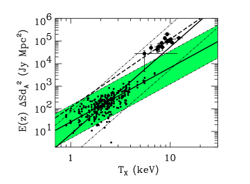
Figure 5: SZ flux decrement at 145 GHz, integrated within $r_{2500}$, vs. the X-ray emission weighted temperature. Symbols and the dashed line are as in Figure 4. The solid lines are the fits to the simulated sample using the least absolute deviation method. Dot-dashed lines show the range $\pm 3D$ where $D$ is the mean absolute deviation, from the fitting relation, of each simulated cluster in the $\Delta S$-direction. The shallower relation, which corresponds to the shaded area, assumes $T_{X}$ as the independent variable, whereas the steeper relation assumes $E(z)\Delta Sd_{A}^{2}$ as the independent variable. The $\pm 3D$ range of the shallower relation has been shaded for clarity. The temperatures of the real clusters are not corrected for the presence of a cooling flow.

The best fit to the simulated cluster sample (the dots in Figure 3) is

$$\log\left(y_{0}\over 10^{-4}\right) = (-0.57\pm 0.01)+$$ (27)

$$+ (0.79\pm 0.02)\log\left[L_{X}\over 10^{44}h^{-2}{\rm erg\ s}^{-1}\right]\;,$$ (28)

in agreement with the self-similar model. We do not attempt to simulate observational error bars on the cluster data extracted from the simulation, because such a detailed analysis is beyond the scope of this paper. Therefore, in the absence of errors on the simulated data, the uncertainties on the fitting parameters we compute are only indicative (e.g. Press et al. 1992, p. 661). An alternative estimate of the uncertainty on this scaling relation is provided by the relative variance on a logarithmic scale $\sigma^{2}=\langle[\log(y_{0})-\log(y_{0}^{\rm fit})]^{2}\rangle$. We find $\sigma=0.10$, comparable to the typical uncertainties of observed $y_{0}$’s. The dotted lines in Figure 3 show the $\pm 3\sigma$ amplitude.

An analogous fit to 17 observed clusters (open circles in Figure 3) drawn from the sample compiled by McCarthy et al. (2003b), mostly based on the sample of Reese et al. (2002), yields the relation: $\log(y_{0}/10^{-4})=(-0.37\pm 0.05)+(0.65\pm 0.04)\log[E^{1/3}(z)L_{X}/10^{44}h^{-2}{\rm erg\ s}^{-1}]$, in reasonable agreement with the self-similar model and our simulated sample. In computing $E(z)$, we assume $\Omega_{0}=0.3$ and $\Omega_{\Lambda}=0.7$.

In passing, we note that the apparent bimodal distribution between simulated and observed data is a consequence of the observational bias of pointing at the very massive clusters: the volume of our simulation box is not large enough to include that many massive clusters.

Despite their small statistical errors, the fit parameters on the real sample should be treated with caution. In fact, the sample of Cooray (1999) (solid circles) yields a shallower relation $\log(y_{0}/10^{-4})=(-0.08\pm 0.05)+(0.47\pm 0.07)\log[E^{1/3}(z)L_{X}/10^{44}h^{-2}{\rm erg\ s}^{-1}]$. The discrepancy between the two observed samples might be statistically meaningless, however, because the probability $q$ of getting a larger $\chi^{2}$ with a sample drawn from a cluster population which obeys either fit to the observed samples is $\la 4\times 10^{-8}$ (Table 1). The small uncertainties claimed for the observed values explain the large $\chi^{2}$’s, which on turn originate the small significance levels $q$. The discovery of possible systematic errors can of course bring the observed samples in better agreement with each other and with a single scaling relation. Indeed the Cooray (1999) sample has 10 out of 14 clusters in common with McCarthy et al. (2003b) sample, but this latter sample have more recent and different measures of $y_{0}$ and, in some cases, of $L_{X}$: these differences might reflect both random and systematic errors.

An intrinsic scatter in the $y_{0}-L_{X}$ scaling relation is in any case expected, due to the simplifying assumptions used to derive $y_{0}$, namely the isothermality of the ICM, the $\beta-$model and the cluster sphericity. It is remarkable that the scatters shown by our simulated clusters and by the observed samples are comparable.

Table 1: Fit parameters to the scaling relations $\log(f_{2}Y)=a+b\log(f_{1}X)$.

$X-Y$		$a$	$b$	$\chi^{2}/\nu$	$q$
$L_{X}-y_{0}$	(1)	$-0.08\pm 0.05$	$0.47\pm 0.07$	4.09	2.5e-8
$f_{1}^{3}=E$	(2)	$-0.37\pm 0.05$	$0.65\pm 0.04$	4.31	3.9e-8
$f_{2}=1$	(4)	$-0.57\pm 0.01$	$0.79\pm 0.02$
$T_{X}-y_{0}$	(1)	$-1.60\pm 0.31$	$1.87\pm 0.31$	1.78	2.5e-2
$f_{1}^{3}=E^{2}$	(2)	$-1.88\pm 0.39$	$2.24\pm 0.39$	1.06	0.39
$f_{2}=1$	(3)	$-2.31\pm 0.54$	$2.79\pm 0.51$	3.03	1.7e-4
	(3a)	$-2.60\pm 0.59$	$3.27\pm 0.60$	6.94	1.3e-13
	(4)	$-1.31\pm 0.01$	$1.55\pm 0.03$
$T_{X}-\Delta S$	(3)	$2.73\pm 0.38$	$2.26\pm 0.38$	0.70	0.76
$f_{1}=1$	(3a)	$2.07\pm 0.42$	$3.02\pm 0.44$	2.30	4.9e-3
$f_{2}=d_{A}^{2}E$	(4)	$1.42\pm 0.04$	$2.41\pm 0.11$
	(4a)	$0.88\pm 0.12$	$3.86\pm 0.19$

(1) Cooray (1999); (2) McCarthy et al. (2003b); (3)/(3a) Benson et al. (2004) with temperatures corrected/not corrected for the presence of a cooling flow; (4) simulated clusters; in the $T_{X}-\Delta S$ relation the fits to the simulated sample are computed with the method of the least mean absolute deviation; (4a) is the fit to the simulated sample assuming $E(z)\Delta Sd_{A}^{2}$, rather than $T_{X}$, as the independent variable. Units: $L_{X}$: $10^{44}h^{-2}{\rm erg\ s}^{-1}$; $T_{X}$: keV; $y_{0}$: $10^{-4}$; $\Delta Sd_{A}^{2}$: Jy Mpc². $\nu$ is the number of degrees of freedom; $q$ is the significance level of $\chi^{2}/\nu$.

Discrepancies among observed samples can also be seen in the relation between $y_{0}$ and the X-ray temperature $T_{X}$ (Figure 4). For the simulated clusters we plot the emission–weighted temperature averaged over the gas particles within $R_{\rm vir}$

$$T_{X}={\sum{n_{e}}_{i}({n_{\rm H}}_{i}+{n_{\rm He}}_{i})\Lambda(T_{i})T_{i}dV_{i}\over\sum{n_{e}}_{i}({n_{\rm H}}_{i}+{n_{\rm He}}_{i})\Lambda(T_{i})dV_{i}}\;.$$ (29)

The simulated clusters yield the relation

$$\log\left(y_{0}\over 10^{-4}\right)=(-1.31\pm 0.01)+(1.55\pm 0.03)\log\left[T_{X}\over{\rm keV}\right],$$ (30)

as expected in the self-similar model. For this relation, the standard deviation on a logarithmic scale is $\sigma=\langle[\log(y_{0})-\log(y_{0}^{\rm fit})]^{2}\rangle^{1/2}=0.10$ (the dotted lines in Figure 4 show the $\pm 3\sigma$ range).

The sample of Cooray (1999) yields a relation close to the self-similar prediction: $\log(y_{0}/10^{-4})=(-1.60\pm 0.31)+(1.87\pm 0.31)\log[E^{2/3}(z)T_{X}/{\rm keV}]$, whereas the sample of McCarthy et al. (2003b) and the more recent sample of Benson et al. (2004), which has 12 out of 15 clusters in common with the McCarthy et al. (2003b) sample, yield considerably steeper relations (Table 1).

Some observed clusters have a central cooling flow. The temperatures of real clusters shown in Figure 4 are corrected for this effect. Neglecting this correction generally decreases the estimate of $T_{X}$ and can substantially change the fit parameters (Table 1). From the statistical point of view, however, we can again draw very little conclusions from most of these $T_{X}-y_{0}$ fits: only the McCarthy et al. (2003b) sample yields a large significance level $q=0.39$.

As we mentioned earlier, the discrepancies that we find among the different observed samples may be due to systematic errors affecting the data analysis. Indeed, Benson et al. (2004) have recently shown how the central $y_{0}$’s calculated from the measurements made with the SuZIE II receiver can be up to 60 per cent higher than the values derived from the BIMA and OVRO interferometers. Therefore, Benson et al. (2004) prefer to use the SZ flux decrement, rather than the central $y_{0}$, as an indicator of the magnitude of the SZ effect.

Figure 5 shows the relation $T_{X}-\Delta S$, where $\Delta S$ is the SZ flux within the circle of radius $r_{2500}$ centered on the cluster: the average mass density within the sphere of radius $r_{2500}$ is 2500 times the critical density. According to Benson et al. (2004), this radius is a suitable choice for the instrumental properties of SuZIE II; moreover, $r_{2500}$ is used in X-ray analyses of clusters (Evrard, Metzler & Navarro, 1996). The simulated sample shows a rather sparse distribution in the $T_{X}-\Delta S$ plane. Therefore we use the least absolute mean deviation method, which, in this case, is more appropriate than the least square fit method, to compute the fitting relation. We find

$$\log\left[\Delta Sd_{A}^{2}\over{\rm Jy\;Mpc}^{2}\right]=(1.42\pm 0.04)+(2.41\pm 0.11)\log\left(T_{X}\over{\rm keV}\right),$$ (31)

as expected in the self-similar model. The observations agree with the self-similar slope only when we use the cooling flow corrected temperatures (sample 3 in Table 1). In this case, however, the normalization of the observed sample is substantially larger than the model. Using the temperatures not corrected for the presence of the cooling flow, as shown in Figure 5 (sample 3a), yields a lower normalization but a substantially different slope. We do not have, however, error bars on our simulated data. Therefore, the fit is sensitive to the choice of the independent variable. Assuming $E(z)\Delta Sd_{A}^{2}$ as the independent variable in the simulated sample (sample 4a) does indeed yield a substantially steeper slope; moreover, the sample variance is large enough to compensate the factor of two difference in the normalization.

In conclusion, our simulated cluster sample seems to provide a reasonable description of the currently observed scaling relations between SZ and X-ray properties. To derive stronger constraints on our simulations of the ICM, however, we should perform more realistic mock observations of SZ clusters, although the disagreement, that we find among the observed samples of SZ clusters, casts some doubts on the robustness of the observed relations available to date.

5 The basic assumptions on the velocity measurements

The measure of the line-of-sight peculiar velocity of clusters with the SZ effects relies on two fundamental assumptions about the physical properties of the ICM: (1) bulk flows of gas clouds within the ICM are negligible and gas and dark matter have the same mean peculiar velocity, and (2) the ICM temperature estimated from the X-ray spectrum is a reliable estimate of the temperature weighted by the electron number density. We now check on these assumptions on turn.

5.1 Velocity bias and internal bulk flows

We might expect that turbulence induced by mergers, gas cooling, galactic winds and stellar feedback can provide substantial contribution to the bulk flow of gas clouds within the ICM (e.g. Inogamov & Sunyaev 2003; Sunyaev, Norman & Bryan 2003; Schuecker et al. 2004). In clusters with low peculiar velocity, these effects can also result in a gas mean velocity quite different from the mean velocity of the dark matter halo. Our simulation, which includes these physical processes, should provide a sample of realistic clusters for the investigation of these effects.

In terms of velocity magnitudes, for each simulated cluster, the three components of the mean velocity of the gas particles within $R_{\rm vir}$, $v_{\rm gas}$, never deviate substantially from the corresponding components of the mean velocity of the dark matter particles, $v_{\rm DM}$: we find a mean absolute deviation, a more robust estimator of the width of a distribution than the standard deviation, $\langle|v_{\rm gas}-v_{\rm DM}|\rangle=18\pm 15$ km s^-1; the maximum value in our sample is $|v_{\rm gas}-v_{\rm DM}|_{\rm max}=88$ km s^-1.

However, in terms of relative velocities, the bias can be substantial. Setting a threshold at $v_{\rm DM}^{t}=100$ km s^-1, we find a mean deviation $\langle\delta\rangle=\langle|(v_{\rm gas}-v_{\rm DM})/v_{\rm DM}|\rangle=0.9\pm 2.2$ for the clusters with $v_{\rm DM}<v_{\rm DM}^{t}$, an order of magnitude larger and with a substantially larger deviation than $\langle\delta\rangle=0.09\pm 0.08$ for the clusters with $v_{\rm DM}>v_{\rm DM}^{t}$. We conclude that we should not expect any relevant systematics from velocity bias when we consider clusters with line-of-sight peculiar velocities larger than $\sim 100$ km s^-1.

We also need to quantify how much the bulk flow of gas clouds within the ICM can affect the peculiar velocity estimate. We consider the velocity maps $v_{ij}=c\beta_{ij}$, where $\beta_{ij}$ is a generic element of the array corresponding to the map computed according to equation (10); therefore, the velocity $v_{ij}$ is a velocity weighted by the electron number density. We first compute the mean $\langle v_{ij}\rangle$ of the $v_{ij}$ values on the pixels within $R_{\rm vir}$ of the cluster centre. This mean agrees with the true $v_{\rm DM}$ (Figure 6): the mean absolute deviation is $\langle|\langle v_{ij}\rangle-v_{\rm DM}|\rangle=31\pm 32$ km s^-1.

Figure 6: Average $\langle v_{ij}\rangle$ of the velocities at the pixel sites vs. the peculiar velocity of the cluster $v_{\rm DM}$. Only pixels within $R_{\rm vir}$ of the cluster centre are included in the calculation of the means. The dotted line is the relation $\langle v_{ij}\rangle=v_{\rm DM}$.

Figure 7: Distribution of the mean absolute deviations between the velocities at the pixel sites and the peculiar velocity of the cluster $v=v_{\rm DM}$ (solid histogram) or the mean velocity of the velocity map $v=\langle v_{ij}\rangle$ (dashed histogram). Only pixels within $R_{\rm vir}$ of the cluster centre are included in the calculation of the means.

For each map, we then compute the mean absolute deviation $\langle|v_{ij}-v|\rangle$ of the velocity values at the pixel sites from $v=v_{\rm DM}$ or $v=\langle v_{ij}\rangle$. Figure 7 shows the distribution of the $\langle|v_{ij}-v|\rangle$’s for all the maps. The average values are $\langle|v_{ij}-v_{DM}|\rangle=119\pm 48$ km s^-1 and $\langle|v_{ij}-\langle v_{ij}\rangle|\rangle=115\pm 45$ km s^-1. We do not expect the two distributions to be different because $\langle|\langle v_{ij}\rangle-v_{\rm DM}|\rangle$ is small. The two samples, with $v_{\rm DM}$ smaller or larger than the threshold $100$ km s^-1, have a $\langle|v_{ij}-v|\rangle$ distribution similar to the complete sample, both when $v=v_{\rm DM}$ and $v=\langle v_{ij}\rangle$. This last result indicates that the velocity bias found above for the slow clusters ($\langle\delta\rangle=0.9\pm 2.2$) is totally due to the bulk flow of gas clouds within the ICM, and not to different mean velocities of gas and dark matter particles. This conclusion also explains why the scatter of $\langle\delta\rangle$ for the slow clusters ($2.2$) is much larger than the scatter for the fast clusters ($0.08$): bulk flows have roughly the same magnitude, independently of the cluster speed.

According to Figure 7, internal bulk flows produce a deviation, from $v_{\rm DM}$, smaller than 200 km s^-1 in 93 per cent of the cases. We conclude that the velocity bias and internal bulk flows set a conservative lower limit of $\sim 200$ km s^-1 to the uncertainty on peculiar velocity measures with the SZ effects (Nagai et al. 2003; Holder 2004), well below the uncertainties of the currently most accurate observations (LaRoque et al. 2003; Benson et al. 2003; Kitayama et al. 2004), but similar to those expected in future measurements at microkelvin sensitivity and arcminute angular resolution (Knox et al., 2004).

Figure 8: Electron density weighted temperature $T_{e}$ vs. X-ray emission–weighted temperature $T_{X}$. Only gas particles within $r_{\rm lim}$ of the cluster centre are considered. Each panel shows the $T_{X}-T_{e}$ relation for a different value of $r_{\rm lim}$, as indicated. The dotted line is the equation $T_{e}=T_{X}$; the solid line is the best fit $T_{e}=a+bT_{X}$. The parameter $a$ is in keV.

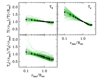
Figure 9: Temperature profiles of the simulated clusters. The upper left (right) panel shows the temperature weighted by the X-ray emission (electron number density). The bottom panel shows the profile of the ratio of the two temperatures. Dotted lines are the individual profiles. Dots with error bars show the mean profiles with 1-$\sigma$ standard deviations.

5.2 Electronic and X-ray temperatures

For all X-ray emitting particles, we can compute an X-ray emission weighted temperature (equation 29) and an electron density weighted temperature

$$T_{e}={\sum{n_{e}}_{i}T_{i}dV_{i}\over\sum{n_{e}}_{i}dV_{i}}\;.$$ (32)

In both equations (29) and (32), the sums run only over the particles within a maximum radius $r_{\rm lim}$.

Note that $T_{e}$ equals a mass-weighted temperature $T_{M}=\sum m_{i}T_{i}/\sum m_{i}$ when the gas is fully ionized, namely ${n_{e}}_{i}\propto\rho_{i}$, which is usually the case for temperatures larger than 0.1 keV.

Figure 8 shows $T_{e}$ vs. $T_{X}$ for different values of $r_{\rm lim}$. The two temperatures are comparable only at the smallest $r_{\rm lim}$, when $T_{e}$ is roughly 10 per cent larger than $T_{X}$ (Mathiesen & Evrard, 2001). At larger $r_{\rm lim}$’s the disagreement increases. In fact, the ICM temperature profile drops at large radii both in real clusters (e.g. De Grandi & Molendi 2002; Kaastra et al. 2003) and in simulations (e.g. Lin et al. 2003; Borgani et al. 2004; Rasia, Tormen & Moscardini 2004).

Figure 9 shows the profiles of our simulated clusters. $T_{X}$ is largely insensitive to $r_{\rm lim}$ because it is proportional to the square of the gas density and is therefore dominated by the emission from the central region. Instead, $T_{e}$ steeply decreases with increasing $r_{\rm lim}$ because it is only proportional to the first power of the electronic gas density.

When $r_{\rm lim}=R_{\rm vir}$, $T_{e}$ can be substantially smaller than $T_{X}$: the mean relation between these two measures of the ICM temperature is $T_{e}/{\rm keV}=0.17+0.69(T_{X}/{\rm keV})$ (Figure 8). Therefore, in spatially poorly resolved clusters, using $T_{X}$ rather than $T_{e}$ can substantially overestimate the peculiar velocity (equations 15 and 22), as we will see in the next section.

Note that here we compute the bolometric temperature. Figure 3 in Borgani et al. (2004) shows that the temperatures estimated by weighting the emissivity in a finite energy band are larger than those obtained by weighting with the bolometric emissivity. Therefore, for real clusters, the $T_{e}-T_{X}$ relation can be shallower and the overestimate of the peculiar velocity more severe. It remains to quantify this trend when a realistic observational procedure is applied to simulated clusters (Mazzotta et al., 2004).

Figure 10: Distributions of the deviations of the estimated line-of-sight velocities from the real velocities of spatially resolved clusters with $v_{DM}>100$ km s^-1. The velocities are estimated with equations (15) where $T_{e}=\langle T_{X}\rangle_{r_{A}}$ (solid histograms), or $T_{e}=\langle T_{e}\rangle_{r_{A}}$ (dashed histograms) and the $\beta$-model parameters are derived from the fit to the X-ray surface brightness. Each panel shows the distributions for a different value of $r_{A}$, as indicated. The other numbers in each panel are the median and the mean absolute deviation from the median of each distribution.

Figure 11: Distributions of the deviations of the estimated line-of-sight velocities from the real velocities of spatially unresolved clusters with $v_{DM}>100$ km s^-1. The velocities are estimated with equations (22) where $\langle T_{e}\rangle_{\theta_{b}}=\langle T_{X}\rangle_{r_{A}}$ (solid histograms), or $\langle T_{e}\rangle_{\theta_{b}}=\langle T_{e}\rangle_{r_{A}}$ (dashed histograms). Each panel shows the distributions for a different value of $r_{A}$, as indicated. The other numbers in each panel are the median and the mean absolute deviation from the median of each distribution.

6 Peculiar velocity measurements

Measuring the peculiar velocity of clusters with the SZ effect requires the separation of the thermal from the kinetic contribution to the total SZ flux. Spatially resolved and unresolved clusters require two different procedures for this separation.

In the former, a model for the ICM distribution is derived from the X-ray surface brightness to estimate the central values of the SZ contributions. In the latter, the beam-averaged SZ contributions are measured without any information on the ICM distribution. To date, only the former case has been applied to observations.

We now consider these two approaches on turn to estimate the systematics that they introduce on the peculiar velocity measurement. Here, we will only consider the physical properties of the ICM and we will not model the instrumental or data reduction problems which affect real observations.

6.1 Resolved clusters: fitting profile method

We perform a rather simple simulation of the observation of individual clusters. Namely, we (1) construct an X-ray surface brightness map from the simulation, (2) derive the gas distribution shape parameters $\beta_{c}$ and $\theta_{c}$ from the X-ray surface brightness profile, (3) compute the SZ fluctuations in the CMB intensity maps $\Delta I(\nu)$ at four different frequencies $\nu=30$, $143$, $217$, and $353$ GHz, (4) derive the central values $\Delta I_{0}(\nu)$ of the radial fits with the shape parameters $\beta_{c}$ and $\theta_{c}$ imposed by the X-ray surface brightness profile, (5) perform a fit to equation (12) by assuming that the four $\Delta I_{0}(\nu)$’s are independent, (6) estimate the peculiar velocity (equation 15) by using the X-ray temperature $T_{X}$ (equation 29) or the electronic temperature $T_{e}$ (equation 32).

In equation (15), $T_{e}$ indicates the central ICM temperature weighted by the electron density. Observationally, one uses the X-ray temperature averaged within the resolution beam. To quantify the effect of the beam size, we compute the temperature with the gas particles within spheres of different radii $r_{A}$.

Figure 10 shows the distribution of the deviations $(v_{\rm est}-v_{\rm DM})/v_{\rm DM}$ of the estimated line-of-sight peculiar velocity $v_{\rm est}$ from the actual cluster velocity $v_{\rm DM}$. The solid and dashed histograms show these deviations when we use $T_{X}$ or $T_{e}$, respectively. We consider the temperatures averaged within four different radii.

The temperature within the smallest radius $0.1R_{\rm vir}$ is the closest to the central temperature that should be used in equation (15). At this radius, both the X-ray and the electronic temperature overestimate the peculiar velocity. The overestimate with $T_{e}$ is more severe, because $T_{e}$ is 10 per cent larger than $T_{X}$ (Figure 9). The incorrect estimate of the peculiar velocity derives from the fact that the gas is neither spherically and smoothly distributed nor isothermal, as assumed when we impose the $\beta$-model to the X-ray surface brightness. In fact, the agreement between estimated and real peculiar velocity does not improve when we use the $\beta$-model parameters derived from the SZ surface brightness, rather than the X-ray surface brightness, despite the fact that the two parameter sets do not generally coincide (e.g. Yoshikawa, Itoh & Suto 1998; Lin et al. 2003).

The radial profile of the X-ray temperature $T_{X}$ decreases less rapidly than the radial profile of $T_{e}$ (Figure 9). Therefore, the peculiar velocity estimate based on $T_{X}$ is rather insensitive to the beam size, whereas the velocity estimated with $T_{e}$ rapidly decreases with $r_{A}$.

The distributions in Figure 10 only include the clusters with $v_{\rm DM}>100$ km s^-1. Including all the clusters leaves the medians unchanged, but substantially extends the tails of the distributions, because, in slow clusters, errors of order a few tens of km s^-1 produce large relative deviations due to the bulk flows internal to the ICM.

In terms of velocity magnitudes, the deviations are comparable, on average, to the systematics due to the internal bulk flows. The upper panels in Figures 12 show the scatter plot between the estimated and the real velocities for all the clusters when $r_{A}=0.1R_{\rm vir}$. The standard deviations are $\sigma=\langle(v_{\rm est}-v_{\rm DM})^{2}\rangle^{1/2}=153$ km s^-1 and 173 km s^-1, when we use the X-ray or the electronic temperatures, respectively.

If our simulated clusters mirror a realistic sample, we expect that, for spatially resolved clusters with peculiar velocity larger than $\sim 100$ km s^-1, the usual assumptions on the ICM physical properties should cause on average a $\sim 10-20$ per cent systematic overestimate of the velocity. For these clusters, the width of the distribution in the upper-left panel of Figure 10 suggests $\sim 50$ per cent as a typical uncertainty on the velocity estimate.

Figure 12: Relation between the estimated and the actual velocity. Upper (lower) panels show spatially resolved (unresolved) clusters. In left (right) panels the ICM temperature is weighted by the X-ray emission (electron number density) of the gas particles within $r_{A}$. The solid line is the $v_{\rm est}=v_{\rm DM}$ relation. The dashed lines indicate the $\pm 3\sigma$ range from the $v_{\rm est}=v_{\rm DM}$ relation, where $\sigma^{2}=\langle(v_{\rm DM}-v_{\rm est})^{2}\rangle$. The numbers in each panels are the standard deviations $\sigma$ in km s^-1.

6.2 Unresolved clusters: aperture method

When the radio/microwave observations do not spatially resolve the cluster, we need to use the equations described in Sect. 2.2. Here, we compute the $y(\mn@boldsymbol{\theta})$ and $b(\mn@boldsymbol{\theta})$ maps, and compute $\Delta S(x)$ by integrating $\Delta I(x)$ over a beam of physical size $2r_{A}(\theta_{b})=d_{A}\theta_{b}$. We then extract $Y(\theta_{b})$ and $B(\theta_{b})$ from the spectral fit. We emphasize that in this case there is no need of any assumption about the ICM spatial distribution.

Figure 11 shows the distributions of the deviations of the estimated line-of-sight velocities from the real velocities for four different aperture radii $r_{A}$. Our maps have $128\times 128$ pixels and are $12R_{\rm vir}$ on a side. Therefore, we choose $r_{A}\geq 0.3R_{\rm vir}$ to avoid the shot-noise due to the small number of pixels in smaller apertures.

When we use the X-ray temperature averaged over the appropriate aperture in equation (22), the larger is the aperture, the larger is the line-of-sight peculiar velocity overestimate (solid histograms). In fact, the ratio of the two integrated SZ components $B(\theta_{b})/Y(\theta_{b})$, in units of the central ratio $b_{0}/y_{0}$, increases by 45 per cent between $r_{A}=0.3$ and $r_{A}=3R_{\rm vir}$, while $T_{X}$ remains basically constant. On the other hand, the rapid decrease of the electron temperature $T_{e}$ with $r_{A}$ compensates the increase of $B(\theta_{b})/Y(\theta_{b})$, and the peculiar velocity estimate is basically unbiased (dashed histogram).

As for the case of spatially resolved clusters, Figure 11 only shows the clusters with $v_{DM}>100$ km s^-1: slower clusters produce longer tails in the distributions but do not vary the central values.

The lower panels in Figure 12 show the extreme case of unresolved clusters, with beam size $r_{A}=3R_{\rm vir}$. Even in this case the standard deviation is $\sigma=\langle(v_{\rm est}-v_{\rm DM})^{2}\rangle^{1/2}<160$ km s^-1 and therefore comparable to the systematic errors due to the internal bulk flows.

Figure 11 clearly shows that, with only the X-ray temperature available, it is essential to have good spatial resolution, in order to have a measure of the ratio $B(\theta_{b})/Y(\theta_{b})$ within a sufficiently small area where $T_{X}$ and $T_{e}$ are comparable. Otherwise the large value of $T_{X}$ can severely overestimate the peculiar velocity.

7 Conclusions

In principle, the evolution of the velocity field on large scales can be measured by detecting the kinetic SZ effect of galaxy clusters. There exist substantial technical difficulties in this measurement due to the weakness of the signal and due to the fact that the kinetic effect does not produce a spectral distortion of the CMB. Nevertheless, a few detections have been claimed to date (Holzapfel et al. 1997; LaRoque et al. 2003; Benson et al. 2003; Kitayama et al. 2004), and more sensitive instruments will make this measurement less problematic in the near future.

The estimate of the peculiar velocity of a cluster from the amplitude of the kinetic SZ effect assumes an isothermal ICM in hydrostatic equilibrium in the cluster potential well. Recent X-ray observations (e.g. Forman et al. 2003) show that the ICM is actually far from this ideal model.

We extracted a sample of 117 fairly realistic galaxy clusters, with mass larger than $10^{14}h^{-1}M_{\odot}$, from an $N$-body hydrodynamical simulation of a large volume of a $\Lambda$CDM cosmological model to estimate the systematic errors, due to the gas bulk flows and ICM temperature estimate, which can affect the measures of the peculiar velocity.

Our simulation reproduces the observed properties of X-ray clusters (Borgani et al. 2004; Ettori et al. 2004) and the distribution of the intracluster light (Murante et al., 2004) reasonably well. Here, we show that our model also reproduces the observed scaling relation between X-ray and SZ properties, namely the X-ray luminosity or the emission-weighted X-ray temperature vs. the central value $y_{0}$ of the Comptonization parameter map. The results of the comparison, between observed and simulated clusters, that we propose here, are not yet fully satisfactory, mostly because of the lack of a uniform sample of clusters observed both in the microwave and X-ray bands.

We then show that if the ICM is not in hydrostatic equilibrium in the cluster potential well, bulk flows of gas within the ICM itself can introduce a systematic error in the estimate of the peculiar velocity. However, this effect is unlikely to be larger than $\sim 200$ km s^-1. Our result, based on a large sample of simulated clusters, provides a robust statistical confirmation of the analyses of Nagai et al. (2003) and Holder (2004) who considered the $N$-body hydrodynamical simulations of only one and three clusters, respectively.

We finally investigate the relevance of the estimate of $T_{e}$, the ICM temperature weighted by the electron number density, in the peculiar velocity measurement. A possibile systematic error originates from the fact that the observed temperature $T_{X}$, which is derived from the X-ray spectrum, might be a biased estimate of $T_{e}$. In the simulations, $T_{X}$ is usually identified with the temperature weighted by the X-ray emission. When averaged within large radii of the cluster centre, $T_{X}$ can overestimate $T_{e}$ by $\sim 20-50$ per cent. If the angular resolution of the radio/microwave observation is too poor to provide a spatially resolved profile of the SZ surface brightness and it only provides an integrated flux, the temperature overestimate propagates into a peculiar velocity overestimate of the same amount.

On the other hand, in the case of clusters which are spatially resolved in the microwave bands, we can use the temperature of the ICM in the central region of the cluster, where $T_{X}$ is comparable to $T_{e}$. For observations which resolve a tenth of the virial radius, the velocity is still overestimated by $10-20$ per cent, because of the assumptions on the spatial and thermal distribution of the ICM, usually parametrized with a $\beta$-model, used to separate the thermal and kinetic SZ components.

Our results rely on the usual assumption that the emission-weighted temperature extracted from the simulations is comparable to the ICM temperature derived from the observed X-ray spectrum. The emission-weighted temperature can however overestimate the spectral temperature by $20-30$ per cent (Mathiesen & Evrard 2001; Mazzotta et al. 2004; Rasia et al. 2004a). This uncertainty makes the identification of the observed $T_{X}$ with $T_{e}$ more problematic, although it seems to alleviate the systematics we find here.

By combining all these results we can set a conservative lower limit of $\sim 200$ km s^-1 (see Figures 7 and 12) to the systematic errors that will affect upcoming measurements of the cluster peculiar velocity with the SZ effect. This limit is comparable to the accuracy expected when the contamination from dusty galaxies and primary CMB anisotropies is considered in radio/microwave observations at microkelvin sensitivity and arcminute angular resolution (Knox et al., 2004). Therefore, the internal ICM bulk flows and its temperature estimate may limit any substantial improvements that could come from more sensitive microwave measurements and more accurate component separations.

We consider the systematic error we find here a lower limit because we identify clusters in the three-dimensional space of the simulation box and analyze their X-ray and SZ properties in two-dimensional projected maps without including instrumental noise and back-/fore-ground sources. Real-world complications can add further systematic errors (Aghanim et al., 2004). More realistic mock observations of SZ clusters are required to design a method to correct for these biases. To accomplish this task one can construct microwave sky maps from $N$-body hydrodynamical simulations (e.g. Schäfer et al. 2004), identify clusters in these maps (e.g. Melin et al. 2004) and analyze the simulated data according to standard observational procedures. This approach will help to quantify how, in a realistic situation, the different systematic errors propagate into the statistical analysis of cluster velocity fields. We plan to investigate this issue in future work.

References

- Aghanim et al. (2001) Aghanim N., Górski K. M., Puget J.-L., 2001, A&A, 374, 1
- Aghanim et al. (2004) Aghanim N., Hansen S. H., Lagache G., 2004, A&A, submitted, astro-ph/0402571
- Atrio-Barandela et al. (2004) Atrio-Barandela F., Kashlinsky A., Mücket J. P., 2004, ApJ, 601, L111
- Benson et al. (2002) Benson A. J., Reichardt C., Kamionkowski M., 2002, MNRAS, 331, 71
- Benson et al. (2003) Benson B. A. et al., 2003, ApJ, 592, 674
- Benson et al. (2004) Benson B. A., Ade P. A. R., Bock J. J., Ganga K. M., Henson C. N., Thompson K. L., Church S. E., 2004, ApJ, submitted, astro-ph/0404391
- Borgani et al. (2004) Borgani S. et al., 2004, MNRAS, 348, 1078
- Carlstrom et al. (2002) Carlstrom J. E., Holder G. P., Reese E. D., 2002, ARA& A, 40, 643
- Cavaliere & Menci (2001) Cavaliere A., Menci N., 2001, MNRAS, 327, 488
- Cohn & Kadota (2004) Cohn J. D., Kadota K., 2004, astro-ph/0409657
- Cooray (1999) Cooray A. R., 1999, MNRAS, 307, 841
- Courteau & Dekel (2001) Courteau S., Dekel A., 2001, in Astrophysical Ages and Times Scales, ASP Conference Series Vol. 245. edited by T. von Hippel, C. Simpson and N. Manset, San Francisco: Astronomical Society of the Pacific, p. 584
- Croft et al. (2001) Croft R. A. C., Di Matteo T., Davé R., Hernquist L., Katz N., Fardal M. A., Weinberg D. H., 2001, ApJ, 557, 67
- da Silva et al. (2001) da Silva A. C., Barbosa D., Liddle A. R., Thomas P. A., 2001, MNRAS, 326, 155
- da Silva et al. (2004) da Silva A. C., Kay S. T., Liddle A. R., Thomas P. A., 2004, MNRAS, 348, 1401
- De Grandi & Molendi (2002) De Grandi S., Molendi S., 2002, ApJ, 567, 1
- Diaferio et al. (2000) Diaferio A., Sunyaev R. A., Nusser A., 2000, ApJ, 533, L71
- Diaferio et al. (2003) Diaferio A., Nusser A., Yoshida N., Sunyaev R. A., 2003, MNRAS, 338, 433
- Diego et al. (2003) Diego J. M., Mohr J., Silk J., Bryan G., 2003, MNRAS, 341, 599
- Dos Santos & Doré (2002) Dos Santos S., Doré O., 2002, A&A, 383, 450
- Eke et al. (1996) Eke V. R., Cole S., Frenk C. S., 1996, MNRAS, 282, 263
- Eke et al. (1998) Eke V. R., Navarro J. F., Frenk C. S., 1998, ApJ, 503, 569
- Ettori et al. (2004) Ettori S., et al., 2004, MNRAS, 354, 111
- Evrard & Henry (1991) Evrard A. E., Henry J. P., 1991, ApJ, 383, 95
- Evrard et al. (1996) Evrard A. E., Metzler C. A., Navarro J. F., 1996, ApJ, 469, 494
- Feldman et al. (2003) Feldman H. A., et al. 2003, ApJ, 596, L131
- Forman et al. (2003) Forman W., et al., 2003, in High Energy Processes and Phenomena in Astrophysics, IAU Symposium 214, astro-ph/0301476
- Forni & Aghanim (2004) Forni O., Aghanim N., 2004, A&A, 420, 49
- Haehnelt & Tegmark (1996) Haehnelt M. G., Tegmark M., 1996, MNRAS, 279, 545
- Hamilton (1998) Hamilton A. J. S., 1998, in The Evolving Universe. Selected Topics on Large-Scale Structure and on the Properties of Galaxies, Dordrecht: Kluwer Academic Publishers, p. 185
- Hansen (2004) Hansen S. H., 2004, MNRAS, 351, L5
- Hansen et al. (2002) Hansen S. H., Pastor S., Semikoz D. V., 2002, ApJ, 573, L69
- Holder (2004) Holder G. P., 2004, ApJ, 602, 18
- Holder et al. (2001) Holder G. P., Haiman Z., Mohr J. J., 2001, ApJ, 560, L111
- Holzapfel et al. (1997) Holzapfel W. L., Ade P. A. R., Church S. E., Mauskopf P. D., Rephaeli Y., Wilbanks T. M., Lange A. E., 1997, ApJ, 481, 35
- Huterer et al. (2004) Huterer D., Kim A., Krauss L. M., Broderick T., astro-ph/0402002
- Inogamov & Sunyaev (2003) Inogamov N. A., Sunyaev R. A., 2003, Astron. Lett., 29, 791
- Itoh et al. (1998) Itoh N., Kohyama Y., Nozawa S., 1998, ApJ, 502, 7
- Kaastra et al. (2003) Kaastra J. S., et al., 2003, A&A, 413, 415
- Kaiser 1991 (1991) Kaiser N., 1991, ApJ, 383, 104
- Kashlinsky & Atrio-Barandela (2000) Kashlinsky A., Atrio-Barandela F., 2000, ApJ, 536, L67
- Kitayama et al. (2004) Kitayama T., et al., 2004, PASJ, 56, 17
- Knox et al. (2004) Knox L., Holder G. P., Church S. E., 2004, ApJ, 612, 96
- LaRoque et al. (2003) LaRoque S. J., Carlstrom J. E., Reese E. D., Holder G. P., Holzapfel W. L., Joy M., Grego L., 2003, ApJ, submitted, astro-ph/0204134
- Lin et al. (2003) Lin W. C., Norman M. L., Bryan G. L., 2003, astro-ph/0303355
- Mather et al. (1999) Mather J. C., Fixsen D. J., Shafer R. A., Mosier C., Wilkinson D. T., 1999, ApJ, 512, 511
- Mathiesen & Evrard (2001) Mathiesen B. F., Evrard A. E., 2001, ApJ, 546, 100
- Matsubara & Szalay (2002) Matsubara T., Szalay A. S., 2002, ApJ, 574, 1
- Mazzotta et al. (2004) Mazzotta P., Rasia E., Moscardini L., Tormen G., 2004, MNRAS, 354, 10
- McCarthy et al. (2003a) McCarthy I. G., Babul A., Holder G. P., Balogh M. L., 2003a, ApJ, 591, 515
- McCarthy et al. (2003b) McCarthy I. G., Holder G. P., Babul A., Balogh M. L., 2003b, ApJ, 591, 526
- Mei & Bartlett (2003) Mei S., Bartlett J. G., 2003, A&A, 410, 767
- Mei & Bartlett (2004) Mei S., Bartlett J. G., 2004, A&A, 425, 1
- Melin et al. (2004) Melin J.-B., Bartlett J. G., Delabrouille J., 2004, astro-ph/0409564
- Moscardini et al. (2002) Moscardini L., Bartelmann M., Matarrese S., Andreani P., 2002, MNRAS, 335, 984
- Murante et al. (2004) Murante G., et al., 2004, ApJ, 607, L83
- Nagai et al. (2003) Nagai D., Kravtsov A. V., Kosowsky A., 2003, ApJ, 587, 524
- Pointecouteau et al. (1998) Pointecouteau E., Giard M., Barret D., 1998, A&A, 336, 44
- Press et al. (1992) Press W. H., Teukolsky S. A., Vetterling W. T., Flannery B. P., 1992, Numerical Recipes in C - The Art of Scientific Computing, second edition, Cambridge University Press
- Rasia et al. (2004a) Rasia E., Mazzotta P., Borgani S., Moscardini L., Dolag K., Tormen G., Diaferio A., Murante G., 2004a, astro-ph/0409650
- Rasia et al. (2004) Rasia E., Tormen G., Moscardini L., 2004b, MNRAS, 351, 237
- Reese et al. (2002) Reese E. D., Carlstrom J. E., Joy M., Mohr J. J., Grego L., Holzapfel W. L., 2002, ApJ, 581, 53
- Rephaeli (1995) Rephaeli Y., 1995, ARA&A, 33, 541
- Schäfer et al. (2004) Schäfer B. M., Pfrommer C., Bartelmann M., Springel V., Hernquist L., 2004, astro-ph/0407089
- Schäfer et al. (2003) Schäfer B. M., Pfrommer C., Zaroubi S., 2003, MNRAS, submitted, astro-ph/0310613,
- Schuecker et al. (2004) Schuecker P., Finoguenov A., Miniati F., Böhringer H., Briel U. G., 2004, A&A, submitted, astro-ph/0404132
- Schulz & White (2003) Schulz A. E., White M., 2003, ApJ, 586, 723
- Sheth & Diaferio (2001) Sheth R.K., Diaferio A., 2001, MNRAS, 322, 901
- Springel & Hernquist (2002) Springel V., Hernquist L., 2002, MNRAS, 333, 649
- Springel & Hernquist (2003) Springel V., Hernquist L., 2003, MNRAS, 339, 312
- Springel et al. (2001) Springel V., Yoshida N., White S. D. M., 2001, NewA, 6, 79
- Sunyaev et al. (2003) Sunyaev R. A., Norman M. L., Bryan G. L., 2003, Astron. Lett., 29, 783
- Sunyaev & Zeldovich (1972) Sunyaev R. A., Zeldovich Ya. B., 1972, Comments Astrophys. Space Phys., 4, 173
- Sutherland & Dopita (1993) Sutherland R. S., Dopita M. A., 1993, ApJS, 88, 253
- Verde et al. (2002) Verde L., Haiman Z., Spergel D. N., 2002, ApJ, 581, 5
- Voit (2004) Voit M., 2004, Rev. Mod. Phys., in press (astro-ph/0410173)
- Weller et al. (2002) Weller J., Battye R. A., Kneissl R., 2002, PhRvL, 88, 231301
- White et al. (2002) White M., Hernquist L., Springel V., 2002, ApJ, 579, 16
- Yoshikawa et al. (1998) Yoshikawa K., Itoh M., Suto Y., 1998, PASJ, 50, 203