HUTP-04/A022

  Abstract
We study the dependence on configuration in momentum space of the primordial 3-point function of density perturbations in several different scenarios: standard slow-roll inflation, curvaton and variable decay models, ghost inflation, models with higher derivative operators and the DBI model of inflation. We define a cosine between the distributions using a measure based on the ability of experiments to distinguish between them. We find that models fall into two broad categories with fairly orthogonal distributions. Models where non-Gaussianity is created at horizon-crossing during inflation and models in which the evolution outside the horizon dominates. In the first case the 3-point function is largest for equilateral triangles, while in the second the dominant contribution to the signal comes from the influence of long wavelength modes on small wavelength ones. We show that, because the distributions in these two cases are so different, translating constraints on parameters of one model to those of another based on the normalization of the 3-point function for equilateral triangles can be very misleading.

 

1 Introduction

Spectacular experimental observations in cosmology caused a certain optimism about our knowledge of the very early Universe. The results are sometimes described as a confirmation of the standard slow-roll inflation paradigm, but this can be rather misleading. What we really know is that all observations are compatible with a scale invariant spectrum of adiabatic perturbations with Gaussian statistics and that these perturbations exist outside the horizon at the time of recombination. These facts are too generic to be considered a proof of the standard picture and in fact non-minimal scenarios or even radically different proposals are still compatible with the data.

The situation will likely change in the near future. There are three basic observables which we consider the most relevant both to confirm or rule out the minimal slow-roll scenario. The experimental limits on all these parameters are getting close to the interesting range, where a distinction among different proposals is possible.

Tilt of the scalar spectrum. A quite generic prediction of slow-roll inflation is the deviation from a completely flat spectrum. This prediction is a consequence of slow-roll itself and it is therefore rather robust. Although the precise number is model-dependent, in most models $|n-1|$ is of order $1/N_{e}$, where $N_{e}$ is the number of e-folds to the end of inflation when relevant scales exit the horizon. Present limits are of order $|n-1|\lesssim 0.05$ (e.g. [2, 3, 4]), so that we are entering in the interesting region. A deviation from a flat spectrum would strongly support the slow-roll inflation picture and it would allow to distinguish it from ‘ghost inflation’ [5] for example, where $|n-1|$ is expected to be negligible. However, if no tilt is detected slow-roll inflation cannot be safely ruled out: it is easy to build models with a tilt as small as we like.

Gravity wave (GW) contribution. The contribution of GWs is directly related to the value of the Hubble constant $H$ during inflation. The detection of a GW signal would therefore point towards models with big vacuum energy ($V^{1/4}\gtrsim 10^{16}\;{\rm GeV}$). Inflationary models fall into two broad categories. Models with small vacuum energy (which is equivalent to a very small $\epsilon$, $\epsilon\ll 1/N_{e}$, as $H/(M_{P}\sqrt{\epsilon})$ is fixed by the spectrum normalization) with totally negligible productions of GWs and models with big vacuum energy (usually with $\epsilon\sim\eta\sim 1/N_{e}$), where the GW contribution should be close to the present experimental limit, $r\lesssim 0.5$ (e.g. [2, 3]) . The distinction is quite sharp because the two categories can also be distinguished by the variation of the inflaton field during inflation: much smaller than the Planck scale in the first case, comparable to the Planck scale in the second. A possible criticism against models with a sensible production of GWs is that a variation of the inflaton field much bigger than $M_{P}$ seems out of control of the effective field theory [6]. Extra dimensional UV completions provide examples in which this is not true [7]. On the other hand models with very small $\epsilon$ have been considered unnatural as they require a hierarchy between the two slow-roll parameters $\epsilon\ll\eta$ [8]. Experiments in the near future will distinguish between the two possibilities. A detection of a GW signal would be of great support for the simplest slow-roll inflation scenario. GWs are in fact usually negligible in models where additional light fields are responsible for density perturbations [9, 10, 11], (see however [12]) in the ekpyrotic/cyclic scenario [13] and in ghost inflation [5].

Non-Gaussianity. The third observable, which is the main subject of this paper, is the deviations from a pure Gaussian statistics, i.e. the presence of a 3-point function. There are two reasons why the study of the 3-point function is relevant. First of all, in a conventional single field model of inflation, the 3-point function can be explicitly calculated as a function of the slow-roll parameters [14, 15]. It turns out to be very small: the primordial fluctuations are Gaussian up to a level of $10^{-6}$ (dimensionless skewness), which is beyond what we can measure in the near future. Any deviation from this prediction is therefore a clear sign of departure from the simplest picture. The 3-point function therefore appears as the optimal smoking gun for many possible scenarios: additional light fields besides the inflaton, imprints of heavy physics through higher dimension operators, ghost inflation, etc. Conversely, if no significant level of non-Gaussianity is found, this will favor the simplest scenario. Also the ekpyrotic and cyclic scenarios, disregarding the open issue of matching the perturbations across the bounce, can give an extremely Gaussian spectrum [16].

Another reason why the detection of the 3-point function would be very exciting is that it potentially contains a lot of information. The 3-point function of the curvature perturbation $\zeta$ in momentum space

$$\langle\zeta_{\vec{k}_{1}}\zeta_{\vec{k}_{2}}\zeta_{\vec{k}_{3}}\rangle$$ (1)

depends on 2 parameters which characterize the shape of the $(\vec{k}_{1},\vec{k}_{2},\vec{k}_{3})$ triangle, while the dependence under rescaling of the triangle is fixed by scale invariance. The purpose of this paper is to show that this function of two parameters contains a lot of information about the source of non-Gaussianity and that it could be useful to distinguish among different models. Moreover we will study how the experimental limits, which are given assuming a particular form of the 3-point function, change if we modify the shape dependence of (1).

There are in principle other observables which could turn out to be relevant, like for example an isocurvature contribution in the perturbations. Unless a conserved quantity such baryon number prevents it, thermal equilibrium is capable of erasing any isocurvature fluctuations imprinted early on, so that it is rather difficult to get generic predictions. Therefore only for the three observables described above we are confident to enter, with the experimental progress in the next few years, in an interesting range. Whatever the results turn out to be we will get further insight into the early cosmology.

In section 2 we will describe the general features of the 3-point function in different models and underline the qualitative differences. In section 3 we plot the different functions and we quantify how “orthogonal” two distributions are. In section 4 we study the effect of projecting the 3d space into a 2d Cosmic Microwave Background (CMB) map and how experimental limits on non-Gaussianity change taking a different shape dependence. We leave to the appendix a discussion about the approximation we used in the 2d analysis. Conclusions are drawn in section 5.

2 Shape dependence in different models

Translational invariance forces the 3-point function (1) to conserve momentum

$$\langle\zeta_{\vec{k}_{1}}\zeta_{\vec{k}_{2}}\zeta_{\vec{k}_{3}}\rangle=(2\pi)^{3}\delta\big{(}\sum_{i}\vec{k}_{i}\big{)}F(\vec{k}_{1},\vec{k}_{2},\vec{k}_{3})\;,$$ (2)

while scaling invariance implies that the function $F$, symmetric in its arguments, is a homogeneous function of degree $-6$

$$F(\lambda\vec{k}_{1},\lambda\vec{k}_{2},\lambda\vec{k}_{3})=\lambda^{-6}F(\vec{k}_{1},\vec{k}_{2},\vec{k}_{3})\;.$$ (3)

Rotational invariance further reduces the number of independent variables to just 2, for example the two ratios $k_{2}/k_{1}$ and $k_{3}/k_{1}$. Note that the function $F$ is real, because the 3-point function in position space cannot change if we change sign to all coordinates.

One interesting form for the function $F$ is the one usually assumed for the analysis of the data (see e.g. [17]). The quantity we observe $\zeta$ is not Gaussian but it contains a non-linear “correction”

$$\zeta(x)=\zeta_{g}(x)-\frac{3}{5}f_{\rm NL}(\zeta_{g}(x)^{2}-\left<\zeta_{g}^{2}\right>)\;,$$ (4)

where $\zeta_{g}(x)$ is Gaussian. Experimental limits are usually put on the scalar variable $f_{\rm NL}$ (). The most stringent limit comes from the WMAP experiment [17]

$$-58<f_{\rm NL}<134\quad{\rm at}\;95\%\;{\rm C.L.}$$ (5)

If we go to Fourier space, eq. (4) implies a function $F$ of the form

$$F_{\rm local}(\vec{k}_{1},\vec{k}_{2},\vec{k}_{3})=2(2\pi)^{4}(-\frac{3}{5}f_{\rm NL}P_{\cal{R}}^{2})\cdot\frac{\sum_{i}k_{i}^{3}}{\prod k_{i}^{3}}\;,$$ (6)

where $P_{\cal{R}}$ is the amplitude of the power spectrum. Currently the best constraint on its amplitude comes from the CMB anisotropy measurement by the WMAP satellite, $P_{\cal{R}}^{1/2}\simeq 4.3\times 10^{-5}$ [2].

Although originally taken as a simple ansatz, this shape dependence turns out to be physically relevant for many models which predict a sensible non-Gaussianity. The reason is that eq. (4) describes (at leading order) the most generic form of non-Gaussianity which is local in real space. This form is therefore expected for models where non-linearities develop outside the horizon. This happens for all the models in which the fluctuations of an additional light field, different from the inflaton, contribute to the curvature perturbations we observe. In this case non-linearities come from the evolution of this field outside the horizon and from the conversion mechanism which transforms the fluctuations of this field into density perturbations. Both these sources of non-linearity give a non-Gaussianity of the form (4) because they occur outside the horizon. Examples of this general scenario are the curvaton models [9], models with fluctuations in the reheating efficiency [10, 11] and multi-field inflationary models [18] ().

Being local in position space, eq. (6) describes correlation among Fourier modes of very different $k$. It is instructive to take the limit in which one of the modes becomes of very long wavelength [14], $k_{3}\rightarrow 0$, which implies, due to momentum conservation, that the other two $k$’s become equal and opposite. The long wavelength mode $\zeta_{\vec{k}_{3}}$ freezes out much before the others and behaves as a background for their evolution. In this limit $F_{\rm local}$ is proportional to the power spectrum of the short and long wavelength modes

$$F_{\rm local}\propto\frac{1}{k_{3}^{3}}\frac{1}{k_{1}^{3}}\;.$$ (7)

This means that the short wavelength 2-point function $\langle\zeta_{\vec{k}_{1}}\zeta_{-\vec{k}_{1}}\rangle$ depends linearly on the background wave $\zeta_{\vec{k}_{3}}$

$$\langle\zeta_{\vec{k}_{3}}\zeta_{\vec{k}_{1}}\zeta_{-\vec{k}_{1}}\rangle\propto\langle\zeta_{\vec{k}_{3}}\zeta_{-\vec{k}_{3}}\rangle\frac{\partial}{\partial\zeta_{\vec{k}_{3}}}\langle\zeta_{\vec{k}_{1}}\zeta_{-\vec{k}_{1}}\rangle\;.$$ (8)

From this point of view we expect that any distribution will reduce to the local shape (6) in the degenerate limit we considered, if the derivative with respect to the background wave does not vanish.

In standard single field slow-roll inflation the limit $k_{3}\rightarrow 0$ is quite easy to predict. As pointed out by Maldacena [14], different points along the background wave are equivalent to shift in time along the inflaton trajectory, so that the derivative with respect to the background wave is proportional to the tilt of the scalar spectrum. This can be explicitly checked in the full expression of the 3-point function [14]

$$F_{\rm stand}(\vec{k}_{1},\vec{k}_{2},\vec{k}_{3})=\frac{1}{8}(2\pi)^{4}P_{\cal{R}}^{2}\cdot\frac{1}{\prod k_{i}^{3}}\left[(3\epsilon-2\eta)\sum_{i}k_{i}^{3}+\epsilon\sum_{i\neq j}k_{i}k_{j}^{2}+8\epsilon\frac{\sum_{i>j}k_{i}^{2}k_{j}^{2}}{k_{t}}\right]\;,$$ (9)

where $\epsilon$ and $\eta$ are the usual slow-roll parameters and $k_{t}\equiv k_{1}+k_{2}+k_{3}$. In the limit $k_{3}\rightarrow 0$ eq. (9) goes as

$$F_{\rm stand}(\vec{k}_{3}\rightarrow 0)\propto 2(\eta-3\epsilon)\frac{1}{k_{1}^{3}}\frac{1}{k_{2}^{3}}=(n_{s}-1)\frac{1}{k_{1}^{3}}\frac{1}{k_{2}^{3}}\;.$$ (10)

As expected the tilt in the spectrum $n_{s}$ fixes the degenerate limit of the 3-point function. Note however that expression (9) is not of the local form (6) but contains contributions which are important for non-degenerate triangles. If we compare expression (6) and (9) and neglect the different shape dependence, we see that standard single-field inflation predicts $f_{\rm NL}$ of order of the slow-roll parameters.

We have seen that the degenerate limit $k_{3}\rightarrow 0$ describes the effect of a slowly-varying background wave on the 2-point function. In many models the correlation is much weaker in this limit than in the local case (6). Physically this means that the correlation is among modes with comparable wavelength which go out of the horizon nearly at the same time. In this case the 3-point function in the degenerate limit is suppressed by powers of $k_{3}$ with respect to the behaviour of eq. (7). We have correlation among modes of comparable wavelength in all models in which the non-Gaussianity is generated by derivative interactions: these interactions become exponentially irrelevant when the modes go out of the horizon because both time and spatial derivatives become small, so that all the correlation is among modes freezing almost at the same time.

One example of this kind of models is obtained if we add higher derivative operators in the usual inflation scenario; the leading operator of this form is

$$\frac{1}{8\Lambda^{4}}(\nabla\phi)^{2}(\nabla\phi)^{2}\;,$$ (11)

where $\phi$ is the inflaton. It is straightforward to calculate the 3-point function after the addition of this operator [20]. The result is

$$F_{\rm h.d.}(\vec{k}_{1},\vec{k}_{2},\vec{k}_{3})= \frac{1}{8}(2\pi)^{4}P_{\cal{R}}^{2}\frac{\dot{\phi}^{2}}{\Lambda^{4}}\cdot$$

$$\cdot\frac{1}{\prod k_{i}^{3}}\left[\frac{1}{k_{t}^{2}}\Big{(}\sum_{i}k_{i}^{5}+\sum_{i\neq j}(2k_{i}^{4}k_{j}-3k_{i}^{3}k_{j}^{2})+\sum_{i\neq j\neq l}(k_{i}^{3}k_{j}k_{l}-4k_{i}^{2}k_{j}^{2}k_{l})\Big{)}\right]\;.$$ (12)

The ratio $\dot{\phi}^{2}/\Lambda^{4}$, where $\dot{\phi}$ is the velocity of the inflaton, is expected to be less than one in the regime in which we can trust an effective field theory description with cut-off $\Lambda$ and neglect the infinite set of higher dimension operators. Therefore the effect cannot be too big: comparing the previous expression with eq. (6) and neglecting the shape dependence we expect roughly $f_{\rm NL}\lesssim 1$, unless we want to enter into the regime where higher order corrections are unsuppressed. It is easy to check that the expression in brackets in eq. (2) vanishes as $k_{3}^{2}$ in the limit $k_{3}\rightarrow 0$ [20]. The correlation is therefore highly suppressed in the degenerate limit with respect to the local shape (6): the additional powers of $k_{3}$ come from the derivatives in the operator (11) acting on the background wave. The correlation is among modes of comparable wavelength, because the higher derivative interaction vanishes exponentially outside the horizon.

A model of inflation based on the Dirac-Born-Infeld (DBI) action has recently been proposed [21, 22]. This model predicts significant non-Gaussianities and gravity waves. The predicted form of the 3-point function is the same as in equation (2), but the level of non-Gaussianity is much bigger because higher derivatives terms are crucial for the inflaton dynamics.

As a final example we consider the 3-point function predicted by ‘ghost inflation’. Without entering into the details of the model [5], we stress that also in this case the 3-point function is generated by a derivative interaction, so that we expect the same qualitative behaviour than in the previous example, with a substantial level of non-Gaussianity. The explicit form of the 3-point function is not illuminating

$$F_{\rm ghost}(\vec{k}_{1},\vec{k}_{2},\vec{k}_{3})= 2\sqrt{2}\;\pi^{31/10}\;\Gamma\big{(}\frac{1}{4}\big{)}^{1/5}\;\beta\;\alpha^{-8/5}P_{\cal{R}}^{8/5}\cdot$$ (13)

$$\cdot\frac{1}{\prod_{i}k_{i}^{3}}2\,{\rm Re}\,\int_{-\infty}^{0}d\eta\;\eta^{-1}F^{*}(\eta)F^{*}\left(\frac{k_{2}}{k_{1}}\eta\right)F^{\prime*}\left(\frac{k_{3}}{k_{1}}\eta\right)k_{3}(\vec{k}_{1}\cdot\vec{k}_{2})+{\rm symm.}$$

where the contour of integration is $\propto(-1-i)$, $\alpha$ and $\beta$ are unknown order one coefficients and

$$F(x)=\sqrt{\frac{\pi}{8}}(-x)^{3/2}H^{(1)}_{3/4}(x^{2}/2)\;.$$ (14)

It can be checked that in the limit $k_{3}\rightarrow 0$ the integral goes like $k_{3}^{2}$. As in the previous example the correlation is therefore suppressed for modes with very different wavelength.

As the explicit expressions of the 3-point functions we showed have progressively become more and more complicated, in the next section we show the explicit plots of the functions, so that their behaviours and differences can be better appreciated.

3 A 3D comparison

Imagine that we measure the density perturbation $\zeta_{\vec{k}_{i}}$ in a 3-dimensional survey. We assume that the 3-point function is of the form

$$\langle\zeta_{\vec{k}_{1}}\zeta_{\vec{k}_{2}}\zeta_{\vec{k}_{3}}\rangle=A\cdot(2\pi)^{3}\delta\big{(}\sum_{i}\vec{k}_{i}\big{)}F(\vec{k}_{1},\vec{k}_{2},\vec{k}_{3})$$ (15)

and we want to use the data to measure the overall amplitude $A$ (). It is easy to check that the best estimator for $A$, in the limit of small non-Gaussianity, is

$$\hat{A}=\frac{\sum_{\vec{k}_{i}}\zeta_{\vec{k}_{1}}\zeta_{\vec{k}_{2}}\zeta_{\vec{k}_{3}}F(\vec{k}_{1},\vec{k}_{2},\vec{k}_{3})/(\sigma^{2}_{k_{1}}\sigma^{2}_{k_{2}}\sigma^{2}_{k_{3}})}{\sum_{\vec{k}_{i}}F(\vec{k}_{1},\vec{k}_{2},\vec{k}_{3})^{2}/(\sigma^{2}_{k_{1}}\sigma^{2}_{k_{2}}\sigma^{2}_{k_{3}})}\;,$$ (16)

where $\sigma^{2}_{k_{i}}$ is the variance of a given mode and the sums run over all triangles in momentum space. This is the estimator with the least variance. Expression (16) naturally defines a scalar product between two distributions $F_{1}$ and $F_{2}$

$$F_{1}\cdot F_{2}\equiv\sum_{\vec{k}_{i}}F_{1}(\vec{k}_{1},\vec{k}_{2},\vec{k}_{3})F_{2}(\vec{k}_{1},\vec{k}_{2},\vec{k}_{3})/(\sigma^{2}_{k_{1}}\sigma^{2}_{k_{2}}\sigma^{2}_{k_{3}})\;.$$ (17)

Its intuitive meaning is clear: if two distributions have a small scalar product, the optimal estimator (16) for one distribution will be very bad in detecting non-Gaussianities with the other shape and vice versa. We will be more quantitative below. But first of all we want to use this scalar product to make meaningful plots of the different shapes we described in the previous section.

As we discussed the function $F$ depends on only two independent variables. We choose them to be $x_{3}\equiv k_{3}/k_{1}$ and $x_{2}\equiv k_{2}/k_{1}$ and we further assume $x_{3}\leq x_{2}$ to avoid considering the same configuration twice. The inequality $x_{3}\geq 1-x_{2}$ follows from the triangular inequality. Looking at eq. (17) we see that in the definition of the scalar product there is a factor $x_{2}^{3}x_{3}^{3}$ coming from the two spectra in the denominator which are approximately scale-invariant. Furthermore a measure $x_{2}x_{3}$ is required to go from the 3D sum over modes to the integral over $x_{2}$ and $x_{3}$. We conclude that the most meaningful quantity to plot is

$$F(1,x_{2},x_{3})\;x_{2}^{2}x_{3}^{2}\;,$$ (18)

so that the integral of the product of two functions we plot gives directly the scalar product.

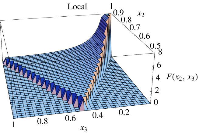
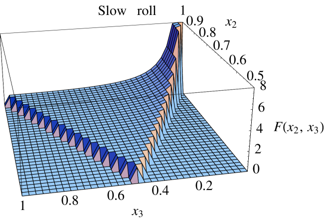
Figure 1: Plot of the function $F(1,x_{2},x_{3})\;x_{2}^{2}x_{3}^{2}$ for the local distribution (6). The figure is normalized to have value 1 for equilateral configurations $x_{2}=x_{3}=1$ and set to zero outside the region $1-x_{2}\leq x_{3}\leq x_{2}$.

Figure 2: Plot of the function $F(1,x_{2},x_{3})\;x_{2}^{2}x_{3}^{2}$ for the usual slow-roll inflation (9) with $\epsilon=\eta=1/30$. The figure is normalized to have value 1 for equilateral configurations $x_{2}=x_{3}=1$ and set to zero outside the region $1-x_{2}\leq x_{3}\leq x_{2}$.

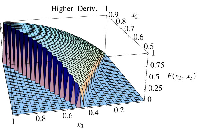
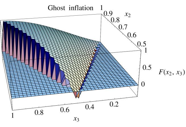
Figure 3: Plot of the function $F(1,x_{2},x_{3})\;x_{2}^{2}x_{3}^{2}$ for non-Gaussianities generated by higher derivative interactions (2) and in the DBI model of inflation [21, 22]. The figure is normalized to have value 1 for equilateral configurations $x_{2}=x_{3}=1$ and set to zero outside the region $1-x_{2}\leq x_{3}\leq x_{2}$.

Figure 4: Plot of the function $F(1,x_{2},x_{3})\;x_{2}^{2}x_{3}^{2}$ for ghost inflation (13). The figure is normalized to have value 1 for equilateral configurations $x_{2}=x_{3}=1$ and set to zero outside the region $1-x_{2}\leq x_{3}\leq x_{2}$.

In figure 2, 2, 4 and 4 we show the shape dependences discussed in the previous section. To avoid showing equivalent configurations twice, the function is set to zero outside the triangular region $1-x_{2}\leq x_{3}\leq x_{2}$. In the first two figures we see, as expected, that the “signal” is concentrated on degenerate triangles $x_{3}\simeq 0$, $x_{2}\simeq 1$, while in the same configuration the third and fourth plots are suppressed. In these two cases the correlation is bigger among modes of comparable wavelength, i.e. equilateral configurations $x_{2}\simeq x_{3}\simeq 1$.

We want to be quantitative about the shape difference of the distributions. From the scalar product (17) we can easily define the cosine between two distributions

$$\cos(F_{1},F_{2})=\frac{F_{1}\cdot F_{2}}{(F_{1}\cdot F_{1})^{1/2}(F_{2}\cdot F_{2})^{1/2}}\;,$$ (19)

which will be a number between $-1$ and 1 (), which tells us how orthogonal two shapes are. If the cosine deviates sensibly from 1, the distinction between two shapes is easy, assuming that a 3-point function has been detected. We numerically calculated the cosine between the 3-point functions we discussed with respect to the local distribution, usually assumed in the data analysis. The results are given in table 1. We see, as expected, that the distributions given by higher derivative terms and ghost inflation are not “collinear” with the local distribution: the cosine deviates significantly from 1. The distribution predicted by the conventional slow-roll scenario is on the other hand quite close to the local distribution, unless $n-1=2(\eta-3\epsilon)=0$ in which case the spectrum is scale invariant and the 3-point function looks quite similar to models with derivative interactions. In going from positive to negative tilt the 3-point function changes sign and close to the transition the cosine with the local model is close to zero.

There is another interesting quantity we can calculate to compare different distributions. For the local distribution we can take $A=f_{\rm NL}$ in eq. (15) and normalize all the other distributions at the equilateral configuration. For every distribution we will have an overall amplitude $f_{\rm NL}^{\rm equil.}$, which can be directly compared to the local case for an equilateral configuration. Imagine now that a 3-dimensional set of data is used to get a limit on $f_{\rm NL}$ for the local distribution. How can we translate this into a limit for $f_{\rm NL}^{\rm equil.}$ for another distribution? We can define a “fudge factor” which converts limit from $f_{\rm NL}$ to $f_{\rm NL}^{\rm equil.}$ for another shape dependence. From eqs. (16) and (17) we easily obtain that the fudge factor $f$ is

$$f(F)\equiv\frac{F\cdot F_{\rm local}}{F_{\rm local}\cdot F_{\rm local}}\;.$$ (20)

The limit on $f_{\rm NL}^{\rm equil.}$ of a given distribution will be the usual $f_{\rm NL}$ parameter divided by $f(F)$. Obviously this procedure is not optimal, because we are using an estimator (16) appropriate for the local distribution to set limits on a different angular dependence. Anyway it is an easy and fast way to get approximate limits without doing the full analysis with a new shape dependence. The fudge factors for the different distributions are given in table 1. We see that the fudge factor is much smaller than 1 for the distribution generated by higher derivative terms and for ghost inflation.

It is interesting to rewrite the definition of $f(F)$ as

$$f(F)=\frac{F\cdot F_{\rm local}}{F_{\rm local}\cdot F_{\rm local}}=\cos(F,F_{\rm local})\left(\frac{F\cdot F}{F_{\rm local}\cdot F_{\rm local}}\right)^{1/2}\;.$$ (21)

We see that the fudge factor is proportional to the cosine between the distributions. This suppression can be eliminated using an optimal estimator for the distribution of interest. The other factor is the ratio between the two norms (i.e. the overall signal) once the functions are normalized at the same value for equilateral triangles; this cannot be changed by the analysis. Obviously for the distributions of fig. (4) and (4) this ratio is quite suppressed as evident from the plots. That explains the smallness of the fudge factors for these two distributions. For example for the ghost model the suppression is a factor of 16, where approximately a factor of 3 comes from the cosine and a factor of 5.5 from the ratio of norms.

Distribution	3d Cosine	3d Factor	2d Cosine	2d Factor
Ghost	0.33	0.06	0.52	0.16
Higher Deriv.	0.45	0.10	0.64	0.24
$\epsilon=1/30$, $\eta=1/30$	0.99	0.73	0.99	0.76
$\epsilon=1/300$, $\eta=1/30$	1.00	1.12	1.00	1.11

Table 1: The 3d and 2d Cosines and Fudge Factors for several different primordial distributions. The values for the DBI model coincide with those of the higher derivative distribution. In the limit $\epsilon\rightarrow 0$ the standard inflation distribution reduces to the local distribution: cosines and fudge factors goes to 1. The 2D numbers are obtained using instrumental noise and band width appropriate for WMAP.

Finally we want to mention the fact that non-linear evolution of modes inside the horizon also creates non-Gaussianity in the density field. It can be observed for example in the local distribution of galaxies (see [23] for a review). These non-Gaussianities are not scale invariant, a fact that can be used to separate them from the primordial contributions [24]. As an example in figure 5 we show the shape of the three point function of the density for $k=0.1\ h\ {\rm Mpc}^{-1}$ for a qualitative comparison with our previous figures of primordial non-Gaussianities. These non-Gaussianities are not only scale dependent, but they also have a different dependence on the triangle shape. The density 3-point function peaks for collinear configurations, that is when the three wavevectors are parallel. This happens because gravity generates density and velocity-divergence gradients that are parallel to the velocity flows [25].

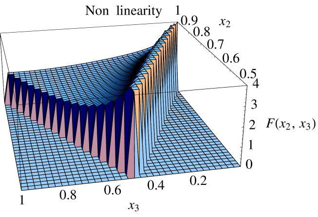
Figure 5: Shape dependence of the density 3-point function for $k=0.1\ h\ {\rm Mpc}^{-1}$. The signal is largest for collinear triangles, when the three wavevectors are parallel. These fluctuations are not scale invariant so both the amplitude and details of the shape are functions of the scale. We present results for a particular wavelength for illustrative purposes.

4 A 2D comparison

Non-Gaussianity in the CMB. The initial curvature perturbations produced during inflation cause corresponding fluctuations in the matter species in the universe. These fluctuations, after being modified by gravitational and hydrodynamical evolution, produce anisotropies in the CMB. Therefore non-Gaussian statistics of the CMB can be used to constrain the non-Gaussian statistics of the underlying perturbations. Most of the fluctuations that we observe in the CMB were imprinted at the epoch of last scattering, around a redshift of $z\sim 1100$. Since the fluctuations were very small at that time it is possible to calculate the radiative transfer of the CMB using linear theory. In this regime any non-Gaussianity in the CMB will be directly related to primordial non-Gaussianity. In reality there are non-linear corrections to the gravitational and hydrodynamical evolution which will produce non-Gaussianities even if the primordial perturbations are Gaussian. One expects such corrections, being of second order in the perturbation, to produce an equivalent $f_{\rm NL}\sim 1$. This is below the current experimental limit but non-linear effects might become important for future experiments. We will ignore them in what follows.

The correspondence between the non-Gaussianities in the CMB sky and those of the primordial curvature is not direct because of the gravitational and hydrodynamical evolution before the epoch of last scattering. Moreover with the CMB one maps a 2-d surface of the universe. The temperature on this surface is a projection of the 3-d curvature perturbations in the surface’s vicinity. This fact introduces further complications if we are interested in the $\vec{k}$ dependence of the primordial 3-point function, not just in its amplitude. In a CMB map one can measure only the components of $\vec{k}$ that are parallel to the plane of the sky, but not the perpendicular one. As a result a measurement of the 3-point function of the CMB temperature for a triangle of one particular shape, will receive contributions from 3-d triangles with a variety of shapes. Moreover the perturbations in the CMB are no longer scale invariant. The evolution inside the horizon imprints several scales in the spectrum, like the scale of the sound horizon or the scale of photon diffusion. These departures from scale invariance, though mild, complicate the analysis.

CMB statistics. As for the curvature fluctuations in 3-d, we will study the 3-point function of the CMB temperature in Fourier space. We will follow the notation of [26]. The temperature fluctuations on the sky are expanded in spherical harmonics,

$$\frac{\Delta T}{T}(\hat{n})=\sum_{lm}a_{lm}Y_{lm}(\hat{n})\;.$$ (22)

We consider the 3-point function $\langle a_{l_{1}m_{1}}a_{l_{2}m_{2}}a_{l_{3}m_{3}}\rangle$ and, assuming rotational invariance, construct the angular averaged bispectrum

$$B(l_{1},l_{2},l_{3})=\sum_{m_{1},m_{2},m_{3}}\left(\begin{array}[]{ccc}l_{1}&l_{2}&l_{3}\\ m_{1}&m_{2}&m_{3}\end{array}\right)\langle a_{l_{1}m_{1}}a_{l_{2}m_{2}}a_{l_{3}m_{3}}\rangle\;.$$ (23)

As we did for the curvature perturbations, we can now define a scalar product in 2-d

$$B_{1}\cdot B_{2}=\sum_{l_{1},l_{2},l_{3}}B_{1}(l_{1},l_{2},l_{3})B_{2}(l_{1},l_{2},l_{3})/(f_{l_{1},l_{2},l_{3}}C_{l_{1}}C_{l_{2}}C_{l_{3}})\;,$$ (24)

where $f_{l_{1},l_{2},l_{3}}$ is a combinatorial factor equal to 1 if the three $l$’s are different, to 2 if two of them are equal and to 6 if all of them are equal. The noise in the denominator of (24) has been calculated in the Gaussian limit and includes instrument noise and beam width in the standard way [26, 27]. The dot product can be used to define a 2-d cosine,

$$\cos(B_{1},B_{2})\equiv\frac{B_{1}\cdot B_{2}}{(B_{1}\cdot B_{1})^{1/2}(B_{2}\cdot B_{2})^{1/2}}\;,$$ (25)

and a 2-d fudge factor,

$$f(B)\equiv\frac{B\cdot B_{\rm local}}{B_{\rm local}\cdot B_{\rm local}}\;.$$ (26)

Calculation of CMB Bispectra. The temperature anisotropies on the sky are linearly related to the underlying curvature perturbations. The contribution to the temperature fluctuations at multipole $l$ from a curvature fluctuation with wavenumber $k$ is encoded in the radiation transfer function $\Delta^{T}_{l}(k)$. In particular we have,

$$\langle a_{l_{1}m_{1}}a_{l_{2}m_{2}}a_{l_{3}m_{3}}\rangle=(4\pi)^{3}i^{l_{1}+l_{2}+l_{3}}\int\frac{d^{3}\vec{k}_{1}}{(2\pi)^{3}}\frac{d^{3}\vec{k}_{2}}{(2\pi)^{3}}\frac{d^{3}\vec{k}_{3}}{(2\pi)^{3}}Y^{*}_{l_{1}m_{1}}(\hat{k}_{1})Y^{*}_{l_{2}m_{2}}(\hat{k}_{2})Y^{*}_{l_{3}m_{3}}(\hat{k}_{3})$$ (27)

$$\times(2\pi)^{3}\delta^{(3)}(\sum_{i}\vec{k}_{i})F(k_{1},k_{2},k_{3})\Delta^{T}_{l_{1}}(k_{1})\Delta^{T}_{l_{2}}(k_{2})\Delta^{T}_{l_{3}}(k_{3})\;.$$

The radiation transfer function $\Delta^{T}_{l}(k)$ can be calculated with publicly available software such as CMBFAST [30]. Expressing the $\delta$ function as an exponential and expanding it in spherical harmonics and Bessel functions we get,

$$\langle a_{l_{1}m_{1}}a_{l_{2}m_{2}}a_{l_{3}m_{3}}\rangle=\int\frac{2k^{2}_{1}dk_{1}}{\pi}\frac{2k^{2}_{2}dk_{2}}{\pi}\frac{2k^{2}_{3}dk_{3}}{\pi}\int d^{2}\hat{x}Y^{*}_{l_{1}m_{1}}(\hat{x})Y^{*}_{l_{2}m_{2}}(\hat{x})Y^{*}_{l_{3}m_{3}}(\hat{x})$$ (28)

$$\times\int\limits^{\infty}_{0}x^{2}dx\;j_{l_{1}}(k_{1}x)j_{l_{2}}(k_{2}x)j_{l_{3}}(k_{3}x)F(k_{1},k_{2},k_{3})\Delta^{T}_{l_{1}}(k_{1})\Delta^{T}_{l_{2}}(k_{2})\Delta^{T}_{l_{3}}(k_{3})\;.$$

In three dimensions, translation invariance forced the three $\vec{k}$’s in the 3-point function to add to zero. In 2-d the equivalent constraint of rotational invariance in enforced by the Gaunt integral

$$\mathcal{G}^{m_{1},m_{2},m_{3}}_{l_{1},l_{2},l_{3}} = \int d^{2}\hat{x}Y_{l_{1}m_{1}}(\hat{x})Y_{l_{2}m_{2}}(\hat{x})Y_{l_{3}m_{3}}(\hat{x})$$ (33)

$$= \sqrt{\frac{(2l_{1}+1)(2l_{2}+1)(2l_{3}+1)}{4\pi}}\left(\begin{array}[]{ccc}l_{1}&l_{2}&l_{3}\\ 0&0&0\end{array}\right)\left(\begin{array}[]{ccc}l_{1}&l_{2}&l_{3}\\ m_{1}&m_{2}&m_{3}\end{array}\right)\;.$$

It forces $l_{1}$, $l_{2}$ and $l_{3}$ to satisfy a triangle inequality. The integral

$$\mathcal{C}_{l_{1},l_{2},l_{3}}(k_{1},k_{2},k_{3})=\int\limits^{\infty}_{0}x^{2}dx\;j_{l_{1}}(k_{1}x)j_{l_{2}}(k_{2}x)j_{l_{3}}(k_{3}x)\;,$$ (34)

determines the strength with which a 3d triangle contributes to a 2d triangle. When considering the 2-point function, the equivalent of eq. (33) is $\delta_{l_{1},l_{2}}\delta_{m_{1},m_{2}}$ and eq. (34) becomes proportional to $\delta^{(1)}(k_{1}-k_{2})$. Using these definitions we can write the reduced CMB bispectrum in a more convenient form

$$B(l_{1},l_{2},l_{3}) =\sqrt{\frac{(2l_{1}+1)(2l_{2}+1)(2l_{3}+1)}{4\pi}}\left(\begin{array}[]{ccc}l_{1}&l_{2}&l_{3}\\ 0&0&0\end{array}\right)$$

$$\!\!\!\!\!\!\!\times\int\frac{2k^{2}_{1}dk_{1}}{\pi}\frac{2k^{2}_{2}dk_{2}}{\pi}\frac{2k^{2}_{3}dk_{3}}{\pi}\mathcal{C}_{l_{1},l_{2},l_{3}}(k_{1},k_{2},k_{3})F(k_{1},k_{2},k_{3})\Delta^{T}_{l_{1}}(k_{1})\Delta^{T}_{l_{2}}(k_{2})\Delta^{T}_{l_{3}}(k_{3})\;.$$

Numerical Challenges. The evaluation of equation (4) is numerically very challenging. It not only involves a four dimensional integral, but both the Bessel functions in eq. (34) and the radiation transfer functions in eq. (4) are very rapidly oscillating. For example the radiation transfers function oscillate when $k$ changes by order the inverse of the distance to the last scattering surface, $\Delta k\sim 1/d_{\rm LSS}$. Moreover the contribution to multipole $l$ comes preferentially from modes with wavenumber $k\sim l/d_{\rm LSS}$. Thus for $l\sim 1000$ the radiation transfer functions have many oscillations in the $k$ range of interest. We can estimate that in order to even crudely calculate the integral in equation (4) the transfer function needs to be evaluated in $200$ values of $k$. Since there are three integrals over $k$ the required number of evaluations is roughly $(200)^{3}\sim 10^{7}$. In addition there is the integral over the three spherical Bessel function, eq. (34), which is extremely difficult to evaluate numerically due to the oscillatory nature of its integrand. Let us assume that it can be done with $10^{3}$ operations. We need to calculate these integrals roughly $l^{3}_{max}$ times because of the sum which appears in the dot product (25). For $l_{max}\approx 1000$ this is $10^{9}$. We must perform roughly $10^{19}$ operations to compute the dot products by brute force.

It is clear that an alternative way to evaluate these integrals must be developed. For the particular case of the local distribution, $F_{\rm local}$ in eq. (6) can be expressed as a product of functions of $k_{1}$, $k_{2}$ and $k_{3}$ separately and the integral in equation (4) can be split and done more easily [26]. We cannot do this in general because some of the distributions we are considering depend of $k_{t}$ and cannot be factorized.

In the appendix we present a technique to evaluate equation (4) using the flat sky approximation. Under this assumption a simple change of variables can eliminate most of the oscillations in the transfer functions and the integral can then be evaluated numerically with little effort.

Results. The results of cosines and fudge factors with respect to the local distribution are listed in Table 1. We used the instrumental noise and beam width appropriate for the WMAP experiment [28], even though we do not expect big differences for other experiments. The first two entries are for ghost inflation and for the 3-point function generated by higher derivative operators (which coincides with the one in the DBI model). We also show the results for the standard slow-roll inflation distribution calculated for different values of the slow-roll parameters.

Table 1 shows that the cosines between distributions calculated for an ideal 3-D experiment and those calculated for a CMB map are quite similar. That is to say, models that are distinguishable in 3-D are also distinguishable in a 2-D survey. For a given 2-D Fourier mode, the components parallel to the plane of the sky of the 3-D modes that contribute to it are fixed, $\vec{k}^{\parallel}=\vec{l}/d_{\rm LSS}$. However Fourier modes with all possible values of the wavevector component perpendicular to the plane of the sky $k_{\perp}$ can contribute. As a result one expects that the configurational dependence of the 3-point function in 2-D be somewhat washed out relative to the 3-D case. Triangles with all different shapes in 3-D contribute to a given triangle in 2-D. This effect however is rather mild as evident in Table 1. The fact that the primordial bispectrum is scale invariant, i.e. its amplitude is proportional to $k^{-6}$, implies that the dominant contribution comes from modes with $k_{\perp}\sim 0$; the information on the shape is conserved. In a sense this is the same reason why we see acoustic peaks in the power spectrum. In that case one could also argue that modes with different wavenumbers $k$ contribute to any given $l$ and thus the acoustic oscillations in the 3-D transfer function would be washed out in the temperature power spectrum. Clearly that only happens to a small degree.

From the table we can infer how the constraints on $f_{\rm NL}$ from the WMAP 1-yr data convert to limits on $f_{\rm NL}^{\rm equil.}$ for different distributions. For example the allowed interval

$$-58<f_{\rm NL}<134\quad{\rm at}\;95\%\;{\rm C.L.}$$ (38)

is approximately degraded to

$$-360<f_{\rm NL}^{\rm equil.}<840\quad{\rm at}\;95\%\;{\rm C.L.}$$ (39)

for the ghost model. The suppression is roughly a factor of 6. A factor of 3 comes from the difference in norms (i.e. the overall signal once the functions are normalized at the equilateral configuration) and a factor of 2 from the cosine. This last piece could be eliminated by optimizing the data analysis.

5 Conclusions

Deviations from Gaussianity could become a very important probe of the early universe physics, responsible for the density inhomogeneities we observe in the universe today. The minimal slow-roll model of inflation predicts negligible non-Gaussianities (at the level of $10^{-6}$) but many of the alternatives predict levels substantially larger.

The discovery of a 3-point function could provide substantial additional information on the mechanisms that generated the non-Gaussianities through its dependence on triangle shape. In this paper we studied that dependence for some of the best motivated alternatives and quantified the observability of the differences in shapes. We concluded that there are broadly two classes of shapes for the 3-point function. In models such as ghost inflation, the DBI model or when there is significant imprint from heavy physics through higher derivative operators, the non-Gaussianity peaks for “equilateral-type” configurations. For models where the non-Gaussianities are produced outside the horizon the shape of the 3-point function peaks in the collapsed triangle limit, when the wavelength of one of the modes is much larger than that of the other two. This limit is well described by the local model.

We quantified these differences by introducing a cosine between the distributions with a measure based on the signal to noise, that is the ability of experiments to distinguish the different shapes. We found that the cosines between distributions are very similar for CMB experiments and ideal 3D experiments, where the full gravitational potential is mapped in three dimensions. We found that the cosine between the local model and the “equilateral-type” models is around 0.3-0.4 in 3D and 0.5-0.6 in 2D. That is to say, the two distributions are quite orthogonal.

The low cosine means that data analysis techniques optimized for one distribution are not optimal for the other. Setting constraints on the local model is computationally much simpler than for the other examples as a result of various tricks developed in the literature [29]. Our results suggest that to fully exploit available and future data one should find ways of extending existing techniques to apply for other 3-point function shapes.

When comparing different models of non-Gaussianity it has become fairly standard to normalize them to have equal amplitude at equilateral configurations. We showed that because the local model has a fairly small signal there while the “equilateral-type” models peak for these configurations, using this method to read off limits for one model based on constraints on another can be quite misleading. For example we found that the constraints on the ghost-inflation model are significantly relaxed. This is mainly because when normalized at the equilateral configurations, the ghost model is significantly less non-Gaussian than the local model, and to a lesser extent because the data analysis is not optimized for the ghost-inflation distribution.

Appendix

In this appendix we present the approximated method we used to calculate the 2d cosines and fudge factors. We will start with the integral solution of the brightness equation [30],

$$\frac{\Delta T}{T}(\hat{n})=\int\frac{d^{3}\vec{k}}{(2\pi)^{3}}\zeta(\vec{k})\int_{0}^{\tau_{0}}d\tau e^{i\vec{k}\cdot\hat{n}(\tau_{0}-\tau)}S(k,\tau)\;,$$ (40)

where $\Delta T(\hat{n})/T$ is the fluctuation in the CMB temperature in the $\hat{n}$ direction, $S(k,\tau)$ is the CMB source function. The source function encodes the effects of the metric perturbations and photon fluctuations, through the integrated Sachs-Wolfe effect, Doppler effect, gravitational redshift, etc.., on the observed CMB.

In the flat sky approximation one considers directions very close to some fiducial direction, and ignores the curvature of the sky taking $\hat{n}$ to lie in the plane perpendicular to the fiducial direction. This is equivalent to approximating the sphere in a neighborhood of a point by the tangent plane at that point. In this limit the equivalent of spherical harmonic transformation becomes simply a Fourier transform. We have

$$a(\vec{l})=\int d^{2}\hat{n}\;e^{-i\vec{l}\cdot\hat{n}}\;\frac{\Delta T}{T}(\hat{n})\;.$$ (41)

We can separate the exponential term in the line of sight integral into two pieces that depend of the wavevectors parallel and perpendicular to the tangent plane,

$$a(\vec{l})=\int\frac{d^{3}\vec{k}}{(2\pi)^{3}}\zeta(\vec{k})\int_{0}^{\tau_{0}}\!d\tau S(k,\tau)\int d^{2}\hat{n}e^{-i\vec{l}\cdot\hat{n}}e^{i\vec{k}^{\parallel}\cdot\hat{n}(\tau_{0}-\tau)}e^{ik^{z}(\tau_{0}-\tau)}\;.$$ (42)

Evaluating the integral over $\hat{n}$ we recover a 2D $\delta$ function that requires $\vec{l}$ to be equal to the projected wavevector $\vec{k^{\parallel}}$ times the distance to the last scattering of the observed photon,

$$a(\vec{l})=\int\frac{d^{3}\vec{k}}{(2\pi)^{3}}\zeta(\vec{k})\int_{0}^{\tau_{0}}\!d\tau S(k,\tau)e^{ik^{z}(\tau_{0}-\tau)}(2\pi)^{2}\delta^{2}(\vec{l}-\vec{k}^{\parallel}(\tau_{0}-\tau))\;.$$ (43)

This approximation will break down when the tangent plane needed to define a mode with wavenumber $l$ has large deviations from the surface of the sphere that defines the last scattering surface (LSS), that is to say when considering large angular scales. Note that we have not assumed that recombination happens instantaneously. Although the source function is strongly peaked around the decoupling time $\tau_{R}$, it has a width $\delta\tau_{R}$ which for our purposes cannot be ignored.

We separate the phase $e^{ik^{z}(\tau_{0}-\tau_{R})}$ in eq. (43), this factor will cancel when we look at n-point correlation functions of $a(\vec{l})$ because of momentum conservation. We have

$$a(\vec{l})=\int\frac{dk^{z}}{2\pi}e^{ik^{z}(\tau_{0}-\tau_{R})}\int d^{2}\vec{k}^{\parallel}\zeta(\vec{k})\int_{0}^{\tau_{0}}d\tau S(k,\tau)e^{ik^{z}(\tau_{R}-\tau)}\delta^{2}(\vec{l}-\vec{k}^{\parallel}(\tau_{0}-\tau))\;.$$ (44)

This allows us to define a radiation transfer function as,

$$\Delta^{T}(l,k_{z})=\int_{0}^{\tau_{0}}\!d\tau S(k,\tau)e^{ik^{z}(\tau_{R}-\tau)}\delta^{2}(\vec{l}-\vec{k}^{\parallel}(\tau_{0}-\tau))\;.$$ (45)

Comparing eq. (45) to the all sky formula [30]

$$\Delta^{T}_{l}(k)=\int^{\tau_{0}}_{0}\!d\tau S(k,\tau)j_{l}[k(\tau_{0}-\tau)]\;,$$ (46)

we can see that spherical Bessel function encapsulates both the 3D to 2D map of the $\delta$ function and the oscillation present in the exponential factor $e^{ik^{z}(\tau_{0}-\tau_{R})}$.

Now we can calculate the bispectrum by taking the ensemble average of a product of three $a(\vec{l})$,

$$\langle a(\vec{l_{1}})a(\vec{l_{2}})a(\vec{l_{3}})\rangle=\int d\tau_{1}d\tau_{2}d\tau_{3}\int\frac{d^{3}\vec{k}_{1}}{2\pi}\frac{d^{3}\vec{k}_{2}}{2\pi}\frac{d^{3}\vec{k}_{3}}{2\pi}\langle\zeta(\vec{k}_{1})\zeta(\vec{k}_{2})\zeta(\vec{k}_{3})\rangle S(k_{1},\tau_{1})S(k_{2},\tau_{2})S(k_{3},\tau_{3})$$

$$\times e^{i(\tau_{R}-\tau_{1})k_{1}^{z}}e^{i(\tau_{R}-\tau_{2})k_{2}^{z}}e^{i(\tau_{R}-\tau_{3})k_{3}^{z}}\delta^{2}(\vec{l}_{1}-\vec{k}^{\parallel}_{1}(\tau_{0}-\tau_{1}))\delta^{2}(\vec{l}_{2}-\vec{k}^{\parallel}_{2}(\tau_{0}-\tau_{2}))\delta^{2}(\vec{l}_{3}-\vec{k}^{\parallel}_{3}(\tau_{0}-\tau_{3}))\;.$$ (47)

Now we use $\langle\zeta(\vec{k}_{1})\zeta(\vec{k}_{2})\zeta(\vec{k}_{3})\rangle=(2\pi)^{3}\delta^{3}(\vec{k}_{123})F(k_{1},k_{2},k_{3})$ and assume that $\delta\vec{k}^{\parallel}\cdot\vec{\nabla}_{k}F(k_{1},k_{2},k_{3})$ is small, where $\delta k^{\parallel}$ is the variation in $k^{\parallel}$ for a given $l$ as the tangent plane sweeps across the width of the last scattering surface. It is clear from geometry that $\delta k^{\parallel}/k^{\parallel}$ will be order $\delta\tau_{R}/\tau_{R}\sim 10^{-2}$. The 3-point functions we are considering do not have sharp features so this assumption will allow us to use an average $k^{\parallel}$ in our evaluation of the primordial bispectrum without introducing a large error. This is equivalent to interchanging the line of sight integral and the integral over Fourier space and evaluating $\vec{k}^{\parallel}$ at $\vec{l}/(\tau_{0}-\tau_{R})$,

$$\langle a(\vec{l}_{1})a(\vec{l}_{2})a(\vec{l}_{3})\rangle=(\tau_{0}-\tau_{R})^{2}\delta^{(2)}(\vec{l}_{123})\!\int\!dk^{z}_{1}dk^{z}_{2}dk^{z}_{3}\delta(k^{z}_{123})F(k_{1}^{\prime},k_{2}^{\prime},k_{3}^{\prime})\tilde{\Delta}^{T}(l_{1},k_{1}^{z})\tilde{\Delta}^{T}(l_{2},k_{2}^{z})\tilde{\Delta}^{T}(l_{3},k_{3}^{z})$$ (48)

where $k^{\prime}$ means $k$ evaluated such that $\vec{k}^{\parallel}=\vec{l}/(\tau_{0}-\tau_{R})$ and

$$\tilde{\Delta}^{T}(l,k^{z})=\int_{0}^{\tau_{0}}\frac{d\tau}{(\tau_{0}-\tau)^{2}}S(\sqrt{(k^{z})^{2}+l^{2}/(\tau_{0}-\tau)^{2}},\tau)e^{ik^{z}(\tau_{R}-\tau)}\;.$$ (49)

Using the definition for the bispectrum, $\langle a(\vec{l}_{1})a(\vec{l}_{2})a(\vec{l}_{3})\rangle=(2\pi)^{2}\delta^{(2)}(\vec{l}_{123})B(l_{1},l_{2},l_{3})$ we get

$$B(l_{1},l_{2},l_{3})=\frac{(\tau_{0}-\tau_{R})^{2}}{(2\pi)^{2}}\int dk^{z}_{1}dk^{z}_{2}dk^{z}_{3}\delta^{(1)}(k^{z}_{123})F(k^{\prime}_{1},k^{\prime}_{2},k^{\prime}_{3})\tilde{\Delta}^{T}(l_{1},k^{z}_{1})\tilde{\Delta}^{T}(l_{2},k^{z}_{2})\tilde{\Delta}^{T}(l_{3},k^{z}_{3})\;.$$ (50)

This formula is completely generic, it can be used to calculate the flat sky bispectrum produced by any primordial perturbation field. It is much easier to handle numerically and was the basis of our evaluation of the dot products presented in Table 1.

In the flat sky limit we have a 2D $\delta$ function which forces the 2D modes to form a closed triangle. In the full sky calculations this is enforced by the Wigner $3j$ symbols of eq. (33).

References

- [1]
- [2] H. V. Peiris et al., “First year Wilkinson Microwave Anisotropy Probe (WMAP) observations: Implications for inflation,” Astrophys. J. Suppl. 148, 213 (2003) [astro-ph/0302225].
- [3] M. Tegmark et al. [SDSS Collaboration], “Cosmological parameters from SDSS and WMAP,” Phys. Rev. D 69, 103501 (2004) [astro-ph/0310723].
- [4] A. C. S. Readhead et al., “Extended Mosaic Observations with the Cosmic Background Imager,” astro-ph/0402359.
- [5] N. Arkani-Hamed, P. Creminelli, S. Mukohyama and M. Zaldarriaga, “Ghost inflation,” JCAP 0404, 001 (2004) [hep-th/0312100].
- [6] D. H. Lyth, “What would we learn by detecting a gravitational wave signal in the cosmic microwave background anisotropy?,” Phys. Rev. Lett. 78, 1861 (1997) [hep-ph/9606387].
- [7] N. Arkani-Hamed, H. C. Cheng, P. Creminelli and L. Randall, “Extranatural inflation,” Phys. Rev. Lett. 90, 221302 (2003) [hep-th/0301218].
- [8] J. Khoury, P. J. Steinhardt and N. Turok, “Great expectations: Inflation versus cyclic predictions for spectral tilt,” Phys. Rev. Lett. 91, 161301 (2003) [astro-ph/0302012].
- [9] D. H. Lyth, C. Ungarelli and D. Wands, “The primordial density perturbation in the curvaton scenario,” Phys. Rev. D 67, 023503 (2003) [astro-ph/0208055].
- [10] G. Dvali, A. Gruzinov and M. Zaldarriaga, “A new mechanism for generating density perturbations from inflation,” Phys. Rev. D 69, 023505 (2004) [astro-ph/0303591].
- [11] G. Dvali, A. Gruzinov and M. Zaldarriaga, “Cosmological Perturbations From Inhomogeneous Reheating, Freeze-Out, and Mass Domination,” Phys. Rev. D 69, 083505 (2004) [astro-ph/0305548].
- [12] L. Pilo, A. Riotto and A. Zaffaroni, “On the amount of gravitational waves from inflation,” astro-ph/0401302.
- [13] See J. Khoury, “A briefing on the ekpyrotic / cyclic universe,” astro-ph/0401579 and references therein.
- [14] J. Maldacena, “Non-Gaussian features of primordial fluctuations in single field inflationary models,” JHEP 0305, 013 (2003) [astro-ph/0210603].
- [15] V. Acquaviva, N. Bartolo, S. Matarrese and A. Riotto, “Second-order cosmological perturbations from inflation,” Nucl. Phys. B 667, 119 (2003) [astro-ph/0209156].
- [16] P. Steinhardt, private communication.
- [17] E. Komatsu et al., “First Year Wilkinson Microwave Anisotropy Probe (WMAP) Observations: Tests of Gaussianity,” Astrophys. J. Suppl. 148, 119 (2003) [astro-ph/0302223].
- [18] F. Bernardeau and J. P. Uzan, “Non-Gaussianity in multi-field inflation,” Phys. Rev. D 66, 103506 (2002) [hep-ph/0207295] and references therein.
- [19] M. Zaldarriaga, “Non-Gaussianities in models with a varying inflaton decay rate,” Phys. Rev. D 69, 043508 (2004) [astro-ph/0306006].
- [20] P. Creminelli, “On non-Gaussianities in single-field inflation,” JCAP 0310, 003 (2003) [astro-ph/0306122].
- [21] E. Silverstein and D. Tong, “Scalar speed limits and cosmology: Acceleration from D-cceleration,” hep-th/0310221.
- [22] M. Alishahiha, E. Silverstein and D. Tong, “DBI in the sky,” hep-th/0404084.
- [23] F. Bernardeau, S. Colombi, E. Gaztanaga and R. Scoccimarro, “Large-scale structure of the universe and cosmological perturbation theory,” Phys. Rept. 367, 1 (2002) [astro-ph/0112551].
- [24] R. Scoccimarro, E. Sefusatti and M. Zaldarriaga, “Probing Primordial Non-Gaussianity with Large-Scale Structure,” astro-ph/0312286.
- [25] R. Scoccimarro, “Cosmological Perturbations: Entering the Non-Linear Regime,” Astrophys. J. 487, 1 (1997) [astro-ph/9612207].
- [26] E. Komatsu, “The Pursuit of Non-Gaussian Fluctuations in the Cosmic Microwave Background,” astro-ph/0206039.
- [27] L. Knox, “Determination of Inflationary Observable by Cosmic Microwave Background Anisotropy Experiments,” Phys. Rev. D 52, 4307 (1995) [astro-ph/9504054].
- [28] C. L. Bennett et al., “First Year Wilkinson Microwave Anisotropy Probe (WMAP) Observations: Preliminary Maps and Basic Results,” Astrophys. J. Suppl. 148, 1 (2003) [astro-ph/0302207].
- [29] E. Komatsu and D. N. Spergel, “Acoustic Signatures In The Primary Microwave Background Bispectrum,” Phys. Rev. D 63, 063002 (2001) [astro-ph/0005036].
- [30] U. Seljak and M. Zaldarriaga, “A Line of Sight Approach to Cosmic Microwave Background Anisotropies,” Astrophys. J. 469, 437 (1996) [astro-ph/9603033].