Constraints on dark energy from Chandra observations of the largest relaxed galaxy clusters

Abstract

We present constraints on the mean dark energy density, $\Omega_{\rm X}$ and dark energy equation of state parameter, $w_{\rm X}$, based on Chandra measurements of the X-ray gas mass fraction in 26 X-ray luminous, dynamically relaxed galaxy clusters spanning the redshift range $0.07<z<0.9$. Under the assumption that the X-ray gas mass fraction measured within $r_{2500}$ is constant with redshift and using only weak priors on the Hubble constant and mean baryon density of the Universe, we obtain a clear detection of the effects of dark energy on the distances to the clusters, confirming (at comparable significance) previous results from Type Ia supernovae studies. For a standard $\Lambda$CDM cosmology with the curvature $\Omega_{\rm K}$ included as a free parameter, we find $\Omega_{\Lambda}=0.94^{+0.21}_{-0.23}$ (68 per cent confidence limits). We also examine extended XCDM dark energy models. Combining the Chandra data with independent constraints from cosmic microwave background experiments, we find $\Omega_{\rm X}=0.75\pm 0.04$, $\Omega_{\rm m}=0.26^{+0.06}_{-0.04}$ and $w_{\rm X}=-1.26\pm 0.24$. Imposing the prior constraint $w_{\rm X}>-1$, the same data require $w_{\rm X}<-0.7$ at 95 per cent confidence. Similar results on the mean matter density and dark energy equation of state parameter, $\Omega_{\rm m}=0.24\pm 0.04$ and $w_{\rm X}=-1.20^{+0.24}_{-0.28}$, are obtained by replacing the CMB data with standard priors on the Hubble constant and mean baryon density and assuming a flat geometry.

1 Introduction

The matter content of the largest clusters of galaxies is thought to provide an almost fair sample of the matter content of the Universe (e.g. White et al. 1993; Eke et al. 1998). The observed ratio of baryonic-to-total mass in such clusters should therefore closely match the ratio of the cosmological parameters $\Omega_{\rm b}/\Omega_{\rm m}$, where $\Omega_{\rm b}$ and $\Omega_{\rm m}$ are the mean baryon and total mass densities of the Universe in units of the critical density. The combination of robust measurements of the baryonic mass fraction in the largest galaxy clusters with accurate determinations of $\Omega_{\rm b}h^{2}$ from cosmic nucleosynthesis calculations (constrained by the observed abundances of light elements at high redshifts) and/or cosmic microwave background (CMB) experiments, with a reliable measurement of the Hubble constant, $H_{0}$, can therefore be used to determine $\Omega_{\rm m}$.

This method for measuring $\Omega_{\rm m}$, which is particularly attractive in terms of the simplicity of its underlying assumptions, was first highlighted by White & Frenk (1991) and subsequently employed by a number of groups (e.g. Fabian 1991, White et al. 1993, David, Jones & Forman 1995; White & Fabian 1995; Evrard 1997; Mohr, Mathiesen & Evrard 1999; Ettori & Fabian 1999; Roussel, Sadat & Blanchard 2000; Allen, Schmidt & Fabian 2002a; Allen et al. 2003; Ettori, Tozzi & Rosati 2003; Sanderson & Ponman 2003; Lin, Mohr & Stanford 2003). In general, these studies have found $\Omega_{\rm m}<1$ at high significance, with recent work favouring $\Omega_{\rm m}\sim 0.3\,h_{70}^{-0.5}$.

Sasaki (1996) and Pen (1997) were the first to describe how measurements of the apparent redshift dependence of the baryonic mass fraction could also, in principle, be used to constrain the geometry and, therefore, dark energy density of the Universe. The geometrical constraint arises from the dependence of the measured baryonic mass fraction values on the assumed angular diameter distances to the clusters. Although theory and cosmological simulations suggest that the baryonic mass fraction in the largest clusters should be invariant with redshift (e.g. Eke et al. 1998), this will only $appear$ to be the case when the reference cosmology used in making the baryonic mass fraction measurements matches the true, underlying cosmology. The first successful application of such a test was carried out by Allen, Schmidt & Fabian (2002a; hereafter ASF02; see also Allen et al. 2003a) using a small sample of X-ray luminous, dynamically relaxed clusters with precise mass measurements, spanning the redshift range $0.1<z<0.5$. These authors found $\Omega_{\rm m}=0.30\pm 0.04$ and $\Omega_{\Lambda}=0.95^{+0.48}_{-0.72}$. A similar analysis was later carried out by Ettori, Tozzi & Rosati (2003) who obtained consistent results using a larger cluster sample that extended to higher redshift, but which included clusters with a wider range of dynamical states.

The baryonic mass content of galaxy clusters is dominated by the X-ray emitting intracluster gas, the mass of which exceeds the mass of optically luminous material by a factor $\sim 6$ (e.g. White et al. 1993; Fukugita, Hogan & Peebles 1998; other mass components in clusters are expected to make only very small contributions to the total baryon budget). Since the emissivity of the X-ray emitting gas is proportional to the square of its density, the gas mass profile in a cluster can be precisely determined from X-ray data. Measuring the $total$ mass profile is more difficult, however, and requires both a direct measurement of the X-ray gas temperature profile and the assumption of hydrostatic equilibrium in the gas. Measurements of the temperature profiles in intermediate-to-high redshift galaxy clusters have only become possible following the launch of the Chandra X-ray Observatory. The exquisite spatial resolution of Chandra makes measuring the temperature profiles of even distant clusters a relatively straightforward task, given sufficient exposure time. The use of the hydrostatic assumption in making the mass and baryonic mass fraction measurements is more problematic, however, and requires a restriction to dynamically relaxed systems when carrying out a cosmological test similar to that described here.

In this paper we present a significant extension to the ASF02 work. The cluster sample is significantly larger and includes 26 X-ray luminous, dynamically relaxed systems spanning the redshift range $0.07<z<0.9$. As well as enhancing the sample, we have also expanded the analysis. We now include a bias factor, $b$, in the X-ray analysis (see also Allen, Schmidt & Bridle 2003), motivated by gas-dynamical simulations, that accounts for the (relatively small amount of) baryonic material expelled from such clusters as they form. We also examine XCDM dark energy models in which the equation of state parameter, $w_{\rm X}$, is allowed to take any constant value. Finally, as well as results based on the Chandra data using simple priors on $\Omega_{\rm b}h^{2}$, $h$ and $b$, we also present results from the combination of Chandra and CMB data. This latter combination is shown to be particularly powerful in constraining the overall dark energy density.

As in ASF02, we report measurements of the X-ray gas mass fraction for two reference cosmologies: an SCDM cosmology with $h=H_{0}/100$$\hbox{${\rm\thinspace km}{\rm\thinspace s}^{-1}\,$}{\rm\thinspace Mpc}^{-1}$$=0.5$, $\Omega_{\rm m}=1$ and $\Omega_{\Lambda}=0$, and a $\Lambda$CDM cosmology with $h=0.7$, $\Omega_{\rm m}=0.3$ and $\Omega_{\Lambda}=0.7$.

2 Observations and data reduction

Table 1: Summary of the Chandra observations. The columns list the target name, observation date, detector used, observation mode and net exposure after all cleaning and screening processes were applied. The targets are listed in RA order.

	Date	Detector	Mode	Exposure (ks)
MACSJ0242.6-2132	2002 Feb 07	ACIS-I	VFAINT	10.2
Abell 383(1)	2000 Nov 16	ACIS-S	VFAINT	18.0
Abell 383(2)	2000 Nov 16	ACIS-I	VFAINT	17.2
MACSJ0329.7-0212	2002 Dec 12	ACIS-I	VFAINT	16.8
Abell 478	2001 Jan 27	ACIS-S	FAINT	39.9
MACSJ0429.6-0253	2002 Feb 07	ACIS-I	VFAINT	19.1
RXJ0439.0+0520	2000 Aug 29	ACIS-I	FAINT	7.6
MACSJ0744.9+3927(1)	2001 Nov 12	ACIS-I	VFAINT	17.1
MACSJ0744.9+3927(2)	2003 Jan 04	ACIS-I	VFAINT	14.5
Abell 611	2001 Nov 03	ACIS-S	VFAINT	34.5
4C55	2004 Jan 03	ACIS-S	VFAINT	77.8
MACSJ0947.2+7623	2000 Oct 20	ACIS-I	VFAINT	9.6
Abell 963	2000 Oct 11	ACIS-S	FAINT	34.8
MS1137.5+6625	1999 Sep 30	ACIS-I	VFAINT	103.8
Abell 1413	2001 May 16	ACIS-I	VFAINT	8.1
ClJ1226.9+3332	2003 Jan 27	ACIS-I	VFAINT	25.7
MACSJ1311.0-0311	2002 Dec 15	ACIS-I	VFAINT	12.0
RXJ1347.5-1145(1)	2000 Mar 03	ACIS-S	VFAINT	8.6
RXJ1347.5-1145(2)	2000 Apr 29	ACIS-S	FAINT	10.0
RXJ1347.5-1145(3)	2003 Sep 03	ACIS-I	VFAINT	49.3
Abell 1835(1)	1999 Dec 11	ACIS-S	FAINT	18.0
Abell 1835(2)	2000 Apr 29	ACIS-S	FAINT	10.3
3C295	1999 Aug 30	ACIS-S	FAINT	17.0
MACSJ1423.8+2404	2003 Aug 18	ACIS-S	VFAINT	112.5
Abell 2029	2000 Apr 12	ACIS-S	FAINT	19.2
MACSJ1532.9+3021(1)	2001 Aug 26	ACIS-S	VFAINT	9.4
MACSJ1532.9+3021(2)	2001 Sep 06	ACIS-I	VFAINT	9.2
MACSJ1621.6+3810	2002 Oct 18	ACIS-I	VFAINT	7.9
MACSJ1720.3+3536	2002 Nov 03	ACIS-I	VFAINT	16.6
MACSJ1931.8-2635	2002 Oct 20	ACIS-I	VFAINT	12.2
MS2137.3-2353(1)	1999 Nov 18	ACIS-S	VFAINT	20.5
MS2137.3-2353(2)	2003 Nov 18	ACIS-S	VFAINT	26.6
MACSJ2229.8-2756	2002 Nov 13	ACIS-I	VFAINT	11.8

2.1 Sample selection

Our sample consists of 26 galaxy clusters spanning the redshift range $0.07<z<0.9$, with X-ray temperatures $kT\mathrel{\hbox to0.0pt{\lower 3.0pt\hbox{$\sim$}\hss}\raise 2.0pt\hbox{$>$}}5$ keV and X-ray luminosities $L_{\rm X,0.1-2.4}\mathrel{\hbox to0.0pt{\lower 3.0pt\hbox{$\sim$}\hss}\raise 2.0pt\hbox{$>$}}10^{45}\,h_{50}^{-2}$${\rm\thinspace erg}{\rm\thinspace s}^{-1}\,$. The clusters exhibit a high degree of dynamical relaxation in their Chandra images (sharp central X-ray surface brightness peaks, regular X-ray isophotes and minimal isophote centroid variations) and show no evidence for a significant loss of hydrostatic equilibrium in X-ray pressure maps and/or gravitational lensing data, where available. The temperature/luminosity cuts avoid complexities associated with variations in the fraction of baryonic matter expelled from the central regions of the clusters during their formation (Eke et al. 1998; Bialek, Evrard & Mohr 2001; it should be possible to relax these cuts in future work, given an improved calibration of the effect from simulations). No quantitative morphological classification procedure was used in the selection of the sample (although the inclusion of such a procedure using e.g. the power ratios method of Buote & Tsai 1995 would be straightforward in future work). Note that the selection function is not required for the determination of cosmological parameters. We simply require accurate mass measurements.

At moderate-to-high redshifts ($z>0.3$) the extension of the sample with respect to ASF02 was achieved primarily through two Large Programs of Chandra observations, lead by L. van Speybroeck and H. Ebeling, of clusters in the Massive Cluster Survey (MACS; Ebeling, Edge & Henry 2001). From relatively short Chandra observations of 53 individual MACS clusters, we identified 12 systems with a high degree of dynamical relaxation (details of the cluster morphologies are discussed by Ebeling et al. 2004, in preparation). One of the clusters, MACSJ1423.8+2404, also has an additional deep Chandra observation which is used here. In addition to the MACS clusters, we have also included archival Chandra data for two other high redshift systems: MS1137.5+6625 ($z=0.782$; Gioia & Luppino 1994) and ClJ1226.9+3332 ($z=0.892$; Ebeling et al. 2001). The central X-ray emission in these clusters is less sharply peaked than most of the systems at lower redshifts (although the central cooling times in the clusters are still only $2-3\times 10^{9}$ yrs however). However, both clusters exhibit regular X-ray morphologies and are the most apparently relaxed, X-ray luminous clusters that we are aware of at such high redshifts. Additional support for the inclusion of MS1137.5+6625 in our study comes from the agreement of the best fitting total mass model determined from the Chandra X-ray data (presented here) and the independent weak lensing study of Clowe et al. (2000). For an SCDM cosmology, the Chandra data are well described by an NFW mass model with $c=3.5^{+1.8}_{-1.5}$ and $r_{\rm s}=185^{+225}_{-75}h^{-1}$ kpc, implying $r_{200}=c\,r_{\rm s}=650^{+180}_{-100}h^{-1}$ kpc. For the same cosmology, Clowe et al. (2000) find $c=4.2$ and $r_{200}\sim 730h^{-1}$ kpc. The effective velocity dispersion corresponding to the best-fit Chandra mass model, $\sigma=1100^{+300}_{-200}$${\rm\thinspace km}{\rm\thinspace s}^{-1}\,$, is also consistent with the observed value of $\sigma=884^{+185}_{-124}$${\rm\thinspace km}{\rm\thinspace s}^{-1}\,$ (Donahue et al. 1999). Although no detailed weak lensing study is available for ClJ1226.9+3332, Maughan et al. (2004) present a temperature map from XMM-Newton observations which supports the identification of this system as a regular, dynamically relaxed cluster, well suited to the present work. The observed velocity dispersion of $\sigma=997^{+285}_{-205}$${\rm\thinspace km}{\rm\thinspace s}^{-1}\,$ (Maughan et al. 2004) is also consistent with the value of $\sigma\mathrel{\hbox to0.0pt{\lower 3.0pt\hbox{$\sim$}\hss}\raise 2.0pt\hbox{$>$}}1000$${\rm\thinspace km}{\rm\thinspace s}^{-1}\,$ inferred from the Chandra data.

At low redshifts ($z<0.3$) the extension of the sample with respect to ASF02 was achieved via a search of the Chandra archive. Two clusters from the ASF02 sample have been dropped from this work: PKS0745-191 ($z=0.103$) was dropped due to difficulties associated with extrapolating the observed profile beyond the restricted Chandra ACIS-S field of view. Abell 2390 ($z=0.230$) was dropped due to dynamical activity which is not localized and cannot easily be excluded from the analysis. The results for both clusters listed in ASF02 are, however, consistent with the analysis presented here.

2.2 Chandra observations

Table 2: The measured X-ray gas mass fractions at $r_{2500}$ (68 per cent confidence limits) for the reference SCDM and $\Lambda$CDM cosmologies. The results for Abell 2029 and 478 have been extrapolated as described in the text. Redshifts for the MACS clusters are from Ebeling et al. (2004, in preparation). A table containing the redshift and $f_{\rm gas}$ data is available from the authors on request.

		SCDM	$\Lambda$CDM
		$f_{\rm gas}h_{50}^{-1.5}$	$f_{\rm gas}h_{70}^{-1.5}$
MACSJ0242.6-2132		$0.175\pm 0.023$	$0.130\pm 0.018$
Abell 383		$0.169\pm 0.011$	$0.122\pm 0.009$
MACSJ0329.7-0212		$0.155\pm 0.019$	$0.119\pm 0.018$
Abell 478		$0.184\pm 0.011$	$0.120\pm 0.008$
MACSJ0429.6-0253		$0.177\pm 0.017$	$0.141\pm 0.015$
RXJ0439.0+0520		$0.137\pm 0.018$	$0.098\pm 0.013$
MACSJ0744.9+3927		$0.155\pm 0.018$	$0.141\pm 0.019$
Abell 611		$0.149\pm 0.017$	$0.111\pm 0.016$
4C55		$0.163\pm 0.009$	$0.115\pm 0.005$
MACSJ0947.2+7623		$0.173\pm 0.019$	$0.130\pm 0.016$
Abell 963		$0.180\pm 0.015$	$0.128\pm 0.012$
MS1137.5+6625		$0.100\pm 0.016$	$0.094\pm 0.014$
Abell 1413		$0.167\pm 0.019$	$0.114\pm 0.013$
ClJ1226.9+3332		$0.114\pm 0.021$	$0.102\pm 0.027$
MACSJ1311.0-0311		$0.094\pm 0.025$	$0.072\pm 0.022$
RXJ1347.5-1145		$0.137\pm 0.009$	$0.108\pm 0.009$
Abell 1835		$0.164\pm 0.012$	$0.112\pm 0.012$
3C295		$0.129\pm 0.019$	$0.106\pm 0.018$
MACSJ1423.8+2404		$0.135\pm 0.011$	$0.113\pm 0.008$
Abell 2029		$0.189\pm 0.011$	$0.121\pm 0.008$
MACSJ1532.9+3021		$0.159\pm 0.017$	$0.114\pm 0.017$
MACSJ1621.6+3810		$0.156\pm 0.034$	$0.131\pm 0.029$
MACSJ1720.3+3536		$0.159\pm 0.024$	$0.123\pm 0.020$
MACSJ1931.8-2635		$0.189\pm 0.025$	$0.145\pm 0.022$
MS2137.3-2353		$0.169\pm 0.010$	$0.124\pm 0.009$
MACSJ2229.8-2756		$0.177\pm 0.018$	$0.139\pm 0.017$

The Chandra observations were carried out using the Advanced CCD Imaging Spectrometer (ACIS) between 1999 August 30 and 2004 Jan 03. The standard level-1 event lists produced by the Chandra pipeline processing were reprocessed using the $CIAO$ (version 3.0.2) software package, including the latest gain maps and calibration products. Bad pixels were removed and standard grade selections applied. Where possible, the extra information available in VFAINT mode was used to improve the rejection of cosmic ray events. For observations carried out with the ACIS-I detector, we have used the Chandra X-ray Center (CXC)/MIT charge transfer inefficiency correction. Time-dependent gain corrections were applied using A. Vikhlinin’s apply_gain routine. The data were cleaned of periods of anomalously high background using the same author’s lc_clean script, using the recommended energy ranges and bin sizes for each detector. The net exposure times for the individual clusters are summarized in Table 1 and vary between 7.6 and 112.5 ks. The total good exposure time is 825.8 ks.

The data have been analysed using the methods described by Allen et al. (2001a, 2002) and Schmidt et al. (2001). In brief, concentric annular spectra were extracted from the cleaned event lists, centred on the peaks of the X-ray emission from the clusters. The spectra were analysed using XSPEC (version 11.3: Arnaud 1996), the MEKAL plasma emission code (Kaastra & Mewe 1993; incorporating the Fe-L calculations of Liedhal, Osterheld & Goldstein 1995) and the photoelectric absorption models of Balucinska-Church & McCammon (1992). The ACISABS model was used to account for time-dependent contamination along the instrument light path. We have allowed for the small amount of extra contamination present in ACIS-I observations by increasing the optical depth of the ACISABS model contaminant by $\Delta\tau=0.14$ at 0.67 keV (A. Vikhlinin, private communication). Only data in the $0.8-7.0$ keV energy range were used for our analysis (the exceptions being the earliest observations of 3C295, Abell 1835 and Abell 2029 where a wider 0.6-7.0 keV band was used). The spectra for all annuli were modelled simultaneously, in order to determine the deprojected X-ray gas temperature profiles under the assumption of spherical symmetry.

For the nearer clusters ($z<0.3$), background spectra were extracted from the blank-field data sets produced by M. Markevitch and available from the CXC. For the more distant systems (and the first observation of Abell 1835, which has an unusually high, but relatively constant, background level) background spectra were extracted from appropriate, source free regions of the target data sets. (We have confirmed that similar results are obtained using the blank-field background data sets throughout.) Separate photon-weighted response matrices and effective area files were constructed for each region studied, using the calibration files appropriate for the period of observation. For the ACIS-I analysis, we have decreased the quantum efficiency at energies below 2 keV by 7 per cent from the nominal value, and then at all energies by a further 8 per cent. This improves the cross-calibration between ACIS-S and ACIS-I observations of clusters in our sample and is consistent with the recommendations of the Chandra calibration team (A. Vikhlinin, private communication).

2.3 Chandra $f_{\rm gas}$ measurements

For the mass modelling, azimuthally-averaged surface brightness profiles were constructed from background subtracted, flat-fielded images with a $0.984\times 0.984$ arcsec² pixel scale ($2\times 2$ raw detector pixels). When combined with the deprojected spectral temperature profiles, the surface brightness profiles can be used to determine the X-ray gas mass profiles (to high precision) and total mass profiles in the clusters. For this analysis, we have used an enhanced version of the image deprojection code described by White, Jones & Forman (1997).

We have parameterized the cluster total mass profiles (luminous plus dark matter) using a Navarro, Frenk & White (1997; hereafter NFW) model with

$$\rho(r)={{\rho_{\rm c}(z)\delta_{\rm c}}\over{({r/r_{\rm s}})\left(1+{r/r_{\rm s}}\right)^{2}}},$$ (1)

where $\rho(r)$ is the mass density, $\rho_{\rm c}(z)=3H(z)^{2}/8\pi G$ is the critical density for closure at redshift $z$, $r_{\rm s}$ is the scale radius, $c$ is the concentration parameter (with $c=r_{200}/r_{\rm s}$) and $\delta_{\rm c}={200c^{3}/3\left[{{\rm ln}(1+c)-{c/(1+c)}}\right]}$. The normalizations of the mass profiles may also be usefully expressed in terms of an effective velocity dispersion, $\sigma=\sqrt{50}r_{\rm s}cH(z)$ (with $r_{\rm s}$ in units of Mpc and $H(z)$ in $\hbox{${\rm\thinspace km}{\rm\thinspace s}^{-1}\,$}{\rm\thinspace Mpc}^{-1}$). Mass models were examined over regular $100\times 100$ grids in the ($r_{\rm s}$,$\sigma$) plane.

Figure 1: The observed X-ray gas mass fraction profiles for the 26 clusters with the radial axes scaled in units of $r_{2500}$. The reference $\Lambda$CDM cosmology is assumed. Note that $f_{\rm gas}(r)$ is an integrated quantity and the error bars on neighbouring points in a profile are correlated.

               

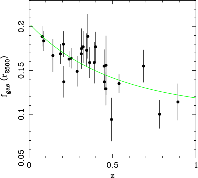
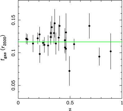
Figure 2: The apparent variation of the X-ray gas mass fraction (with root-mean-square $1\sigma$ errors) as a function of redshift for the reference (a: left panel) SCDM and (b: right panel) $\Lambda$CDM cosmologies. The grey curve in (a) shows the predicted $f_{\rm gas}(z)$ behaviour for the best-fitting model cosmology with $\Omega_{\rm m}=0.25$ and $\Omega_{\Lambda}=0.96$ (see Section 3.2). Clusters at higher redshifts appear to have lower gas mass fractions because the SCDM cosmology underestimates the relative distances to these systems. The curve in (b) shows the best-fitting constant value.

In determining the results on the X-ray gas mass fraction, $f_{\rm gas}$, we have adopted a canonical radius of $r_{2500}$, within which the mean mass density is 2500 times the critical density of the Universe at the redshifts of the clusters. The $r_{2500}$ values are determined directly from the Chandra data, with confidence limits calculated from the $\chi^{2}$ grids and are (in general) well-matched to the outermost radii at which reliable temperature measurements can be made from the Chandra data.

Fig. 1 shows the observed $f_{\rm gas}(r)$ profiles for the 26 clusters in our sample, determined from the Chandra data using the reference $\Lambda$CDM cosmology. Although some variation is present from cluster to cluster, particularly at small radii, the profiles tend towards a universal value at $r_{2500}$. (We note that the cluster with the most discrepant $f_{\rm gas}(r)$ profile and highest $f_{\rm gas}$ value at small radii is MACSJ1532.9+3021, which exhibits an unusually high ellipticity in its innermost regions. 4C55 also exhibits a high ellipticity and isophote shifts at small radii and has the second highest $f_{\rm gas}$ value at $0.1r_{2500}$. Both clusters appear relaxed at larger radii, however, and their $f_{\rm gas}$ profiles have recovered to the ‘universal’ form by $r_{2500}$.) Table 2 lists the results on the X-ray gas mass fractions at $r_{2500}$ for the reference SCDM and $\Lambda$CDM cosmologies. Taking the weighted mean of the $\Lambda$CDM results we obtain ${\bar{f}_{\rm gas}}=0.1173\pm 0.0022\,h_{70}^{-1.5}$.

In calculating the total baryonic mass in the clusters, we assume that the optically luminous baryonic mass in galaxies scales as $0.19h^{0.5}$ times the X-ray gas mass. This result is based on detailed studies of nearby and intermediate redshift clusters (White et al. 1993, Fukugita, Hogan & Peebles 1998; see also Voevodkin & Vikhlinin 2004) and corresponds to $\sim 16$ per cent of the X-ray gas mass. Uncertainties in this correction have a negligible impact on the overall error budget. Other sources of baryonic matter in the clusters are expected to make very small contributions to the total mass and are ignored.

We note that the Chandra data for Abell 478 and 2029 do not extend quite to $r_{2500}$. For these clusters, we measure $f_{\rm gas}$ directly at $r=0.75\,r_{2500}$ for the SCDM cosmology or $r=0.70\,r_{2500}$ for the $\Lambda$CDM cosmology and extrapolate the results to $r_{2500}$ using the median $f_{\rm gas}(r)$ profile determined from Fig. 1. This extrapolation results in corrections to the directly measured $f_{\rm gas}$ values of $\sim 5$ per cent. To be conservative, we have included a 5 per cent systematic uncertainty in the tabulated $f_{\rm gas}$ measurements for Abell 478 and 2029 to allow for uncertainties in this extrapolation.

Fig. 2 shows the $f_{\rm gas}$ values as a function of redshift for the reference SCDM and $\Lambda$CDM cosmologies. Whereas the results for the $\Lambda$CDM cosmology are consistent with a constant $f_{\rm gas}$ value ($\chi^{2}=22.7$ for 25 degrees of freedom) the results for the reference SCDM cosmology indicate an apparent drop in $f_{\rm gas}$ as the redshift increases. The $\chi^{2}=61.8$ obtained from a fit to the SCDM data with a constant model indicates that the SCDM cosmology is inconsistent with the expectation that $f_{\rm gas}(z)$ should be constant.

2.4 CMB analysis

Our analysis of CMB observations uses the WMAP temperature (TT) data for multipoles $l<900$ (Hinshaw et al. 2003) and temperature-polarization (TE) data for $l<450$ (Kogut et al. 2003). To extend the analysis to higher multipoles (smaller scales), we also include data from the Cosmic Background Imager (CBI; Pearson et al. 2003) and Arcminute Cosmology Bolometer Array Receiver (ACBAR; Kuo et al. 2003) for $l>800$. The comparison of model angular power spectra with the WMAP data employs the likelihood calculation routines released by the WMAP team (Verde et al. 2003).

Our analysis of the CMB data uses the CosmoMC code. This in turn uses CAMB (Lewis, Challinor & Lasenby 2000), which is based on CMBFAST (Seljak & Zaldarriaga 1996), to generate the CMB and matter power spectrum transfer functions, and a Metropolis-Hastings Markov Chain Monte Carlo (MCMC) algorithm to explore parameter space. We used the covariance matrix of the parameters calculated from an initial set of test runs to improve sampling efficiency (see Lewis & Bridle 2002 for more details).

We have fitted the data using an extended XCDM cosmological model with eight free parameters: the physical dark matter and baryon densities in units of the critical density, the curvature $\Omega_{\rm K}$, the Hubble constant, the dark energy equation of state parameter, the recombination redshift (at which the reionization fraction is a half, assuming instantaneous reionization), the amplitude of the scalar power spectrum and the scalar spectral index. We also examined a standard $\Lambda$CDM model in which we fixed $w_{\rm X}=-1$. In all cases, we have assumed an absence of tensor components and included uniform priors $30<H_{0}$$\hbox{${\rm\thinspace km}{\rm\thinspace s}^{-1}\,$}{\rm\thinspace Mpc}^{-1}$$<100$ and $-4<w_{\rm X}<1$. (Tests in which tensor components were included with $\Lambda$CDM models lead to similar results on dark energy, but took much longer to compute.)

The analysis was carried out on the Cambridge X-ray group Linux cluster. For each model we accumulated a total of at least $10^{6}$ correlated samples in 10 separate chains. We satisfied ourselves that the chains had converged by ensuring that consistent final results were obtained from numerous small subsets of the chains. In all cases, we allowed a conservative burn-in period of $10^{4}$ samples for each chain.

3 Cosmological analysis

3.1 Dark energy models

We have considered two separate dark energy models in our analysis: standard $\Lambda$CDM and the extended XCDM parameterization. Our definitions of the relevant quantities closely follow Peebles & Ratra (2003) and we refer the reader to that work for a discussion of the underlying assumptions.

The Friedmann equation, which relates the first time derivative of the scale factor of the Universe, $a$, to the total density can be conveniently expressed as $({\dot{a}}/a)^{2}\,$=$\,H(z)^{2}\,$= $H_{0}^{2}E(z)^{2}$, where

$$E(z)=\sqrt{\Omega_{\rm m}(1+z)^{3}+\Omega_{\rm X}f(z)+\Omega_{\rm K}(1+z)^{2}}$$ (2)

Here $\Omega_{\rm X}$ is the dark energy density and $f(z)$ its redshift dependence. (We have ignored the density contribution from radiation and relativistic matter.) For $\Lambda$CDM cosmologies, the dark energy density is constant and $f(z)=1$. Within the extended XCDM dark energy parametrization, the pressure is related to the density as $p_{\rm X}=w_{\rm X}\rho_{\rm X}$ so that for constant $w_{\rm X}$, the dark energy density scales as $\rho_{\rm X}\propto a^{-3(1+w_{\rm X})}$ and $f(z)=(1+z)^{3(1+w_{\rm X})}$. We note that for $w_{\rm X}<-1/3$ the dark energy makes a positive contribution to the acceleration of the expansion of the universe. For $w_{\rm X}<-1$ the dark energy density is increasing with time.

Our analysis of Chandra $f_{\rm gas}$ data requires the angular diameter distances to the clusters which are defined as

$$d_{A}=\frac{c}{H_{0}(1+z)\sqrt{\Omega_{\rm K}}}\,\sinh\left(\sqrt{\Omega_{\rm K}}\int_{0}^{z}{dz\over E(z)}\right).$$ (3)

3.2 Analysis of the $f_{\rm gas}$ data

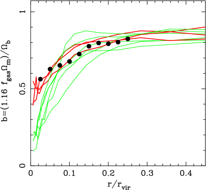
Figure 3: The X-ray bias factor, $b$ (the enclosed baryon fraction relative to the universal value) as a function of radius in units of the virial radius $r_{\rm vir}$, from the simulations of Eke et al. (1998). The simulated clusters have similar masses to the systems studied here. The results for the three most dynamically relaxed clusters in the simulations are shown as darker curves. The solid circles mark the median profile determined from the Chandra observations, scaled from Fig. 1 assuming $\Omega_{\rm m}=0.25$, $\Omega_{\rm b}=0.0413$ and $r_{2500}=0.25\,r_{\rm vir}$. Beyond a radius $r>0.2r_{\rm vir}$, the simulated clusters exhibit consistent, relatively flat $b$ profiles. At $r=0.25r_{\rm vir}$, a radius comparable to the measurement radius of the Chandra observations, the simulations give $b=0.824\pm 0.033$.

The differences between the shapes of the $f_{\rm gas}(z)$ curves in Figs. 2(a) and (b) reflect the dependence of the measured $f_{\rm gas}(z)$ values on the angular diameter distances to the clusters: $f_{\rm gas}\propto(1+z)^{2}d_{\rm A}^{1.5}$. Under the assumption (Section 1) that $f_{\rm gas}$ should, in reality, be constant with redshift, simple inspection of Fig. 2 clearly favours the $\Lambda$CDM over the SCDM cosmology.

To determine constraints on the relevant cosmological parameters, we have fitted the $f_{\rm gas}(z)$ data in Fig. 2(a) with a model that accounts for the expected apparent variation in $f_{\rm gas}(z)$ as the underlying cosmology is varied. (We choose to work with the SCDM data as our reference cosmology, although similar results can be derived using the $\Lambda$CDM data set.) Note that the $f_{\rm gas}(r)$ profiles exhibit only small variations around $r_{2500}$ so changes in $r_{2500}$ as the cosmology is varied can be ignored. The model function fitted to the data is

$$f_{\rm gas}^{\rm SCDM}(z)=\frac{b\,\Omega_{\rm b}}{\left(1+0.19\sqrt{h}\right)\Omega_{\rm m}}\left[\frac{d_{\rm A}^{\rm SCDM}(z)}{d_{\rm A}^{\rm mod}(z)}\right]^{1.5},$$ (4)

where $d_{\rm A}^{\rm mod}(z)$ and $d_{\rm A}^{\rm SCDM}(z)$ are the angular diameter distances to the clusters in the current model and reference SCDM ($h=0.5$) cosmologies. Note that although variations in the dark energy density affect only the $shape$ of the $f_{\rm gas}(z)$ curve, the normalization depends on $\Omega_{\rm m}$, $\Omega_{\rm b}$, $h$ and $b$, where $b$ is a bias factor motivated by gasdynamical simulations which suggest that the baryon fraction in clusters is slightly lower than for the universe as a whole (e.g. Eke, Navarro & Frenk 1998; Bialek et al. 2001). We use the results of Eke et al. (1998) from simulations of 10 clusters of similar masses to the observed systems to constrain $b$. Excluding the data for the most dynamically active cluster in that study (recall that the $f_{\rm gas}$ data are drawn from Chandra observations of dynamically relaxed systems), the simulated clusters show consistent, relatively flat baryonic mass fraction profiles for radii $r>0.2r_{\rm vir}$ (Fig 3). At $r=0.25r_{\rm vir}$, a radius comparable to the measurement radius for the Chandra observations, the simulations of Eke et al. (1998) give $b=0.824\pm 0.033$.

We note the excellent agreement between the median, scaled $f_{\rm gas}(r)$ profile determined from the Chandra data (shown as dark circles in Fig 3) and the simulated profiles for the three most relaxed clusters in the study of Eke et al. (1998; the darker curves in Fig 3). This agreement supports the use of the simulations in estimating the bias factor at $r_{2500}$. Note also that the simulations of Eke et al. (1998) indicate negligible evolution of the bias parameter (measured within $r\sim 0.5r_{\rm vir}$) over the redshift range considered here.

For our analysis of the Chandra $f_{\rm gas}$ data alone, we employ simple Gaussian priors on $\Omega_{\rm b}h^{2}$ and $h$. Two separate sets of priors were used: ‘standard’ priors with $\Omega_{\rm b}h^{2}=0.0214\pm 0.0020$ (Kirkman et al. 2003) and $h=0.72\pm 0.08$ (Freedman et al. 2001), and ‘weak’ priors in which we triple the nominal uncertainties to give $\Omega_{\rm b}h^{2}=0.0214\pm 0.0060$ and $h=0.72\pm 0.24$. (No priors on $\Omega_{\rm b}h^{2}$ and $h$ are assumed in the combined analysis of $f_{\rm gas}$ and CMB data; Section 3.3.)

We assume a Gaussian prior on $b$. The rms fractional deviation in $b$ from the simulations of Eke et al. (1998; $\sim 4$ per cent) was added in quadrature to a nominal 10 per cent systematic uncertainty associated with the overall normalization of the $f_{\rm gas}(z)$ curve. This allows for residual uncertainties associated with the simulations and/or the calibration of the Chandra instruments. Thus, for the analysis of the $f_{\rm gas}$ data alone using the standard priors, the $\chi^{2}$ value for any particular model is

$$\chi^{2} = \left(\sum_{i=1}^{26}\frac{\left[f_{\rm gas}^{\rm SCDM}(z_{\rm i})-f_{\rm gas,\,i}\right]^{2}}{\sigma_{f_{\rm gas,\,i}}^{2}}\right)$$

$$+\left(\frac{\Omega_{\rm b}h^{2}-0.0214}{0.0020}\right)^{2}+\left(\frac{h-0.72}{0.08}\right)^{2}+\left(\frac{b-0.824}{0.089}\right)^{2}.$$ (5)

Here $f_{\rm gas,\,i}$ and $\sigma_{f_{\rm gas,\,i}}$ are the observed values and symmetric rms errors for the SCDM cosmology from Table 2. Note that we have not accounted for the intrinsic cluster-cluster scatter in $b$ explicitly. However, the simulations suggest that this scatter is small when compared with the statistical uncertainties in the $f_{\rm gas}$ measurements.

3.3 Combination of $f_{\rm gas}$ and CMB constraints

For the combined Chandra+CMB analysis, we importance sample the MCMC results from the CMB analysis, folding in the $f_{\rm gas}$ constraints (Allen, Schmidt & Bridle 2003). Each of the MCMC samples from the CMB analysis provides a value for $\Omega_{\rm m}$, $\Omega_{\rm X}$, $w_{\rm X}$, $H_{0}$ and $\Omega_{\rm b}h^{2}$. Using these values, we fit the $f_{\rm gas}(z)$ data with the model described by Equation 4, including the same Gaussian prior on the bias factor, including the allowance for systematic uncertainties in the normalization of the curve. This provides a $\chi^{2}$ value for each of the MCMC samples. The weight of the MCMC sample is then multiplied by $e^{-\chi^{2}/2}$.

4 Cosmological constraints

4.1 Results for the $\Lambda$CDM cosmology

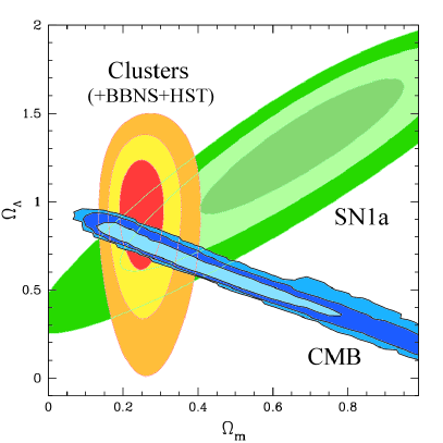
Figure 4: The 68.3, 95.4 and 99.7 per cent (1, 2 and 3$\sigma$) confidence constraints in the $\Omega_{\rm m},\Omega_{\Lambda}$ plane obtained from the analysis of the cluster $f_{\rm gas}$ data using standard priors on $\Omega_{\rm b}h^{2}$ (Kirkman et al. 2003) and $h$ (Freedman et al. 2001). Also shown are the independent results obtained from CMB data using a weak uniform prior on $h$ ($0.3<h<1$), and Type 1a supernovae data (Tonry et al. 2003). A $\Lambda$CDM cosmology is assumed with the curvature, $\Omega_{\rm K}$, included as a free parameter in the analysis.

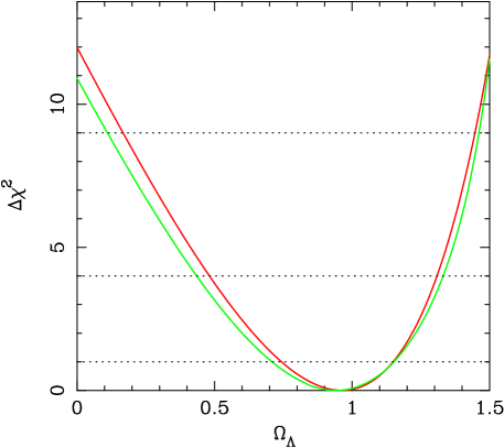
Figure 5: The marginalized constraints on $\Omega_{\Lambda}$ obtained from the Chandra $f_{\rm gas}$ data using the standard (dark curve) and weak (light curve) priors on $\Omega_{\rm b}h^{2}$ and $h$. The dotted lines mark the formal 1, 2 and 3$\sigma$ limits (see text for details). The curvature is a free parameter in the analysis.

Figure 6: The 68.3, 95.4 and 99.7 per cent confidence constraints in the $\Omega_{\rm m},\Omega_{\Lambda}$ plane obtained from the analysis of the combined $f_{\rm gas}$+CMB data set using the $\Lambda$CDM model. We find marginalized 68 per cent confidence limits of $\Omega_{\rm m}=0.28^{+0.05}_{-0.04}$ and $\Omega_{\Lambda}=0.73^{+0.04}_{-0.03}$, with $\Omega_{\rm K}=-0.01\pm 0.02$.

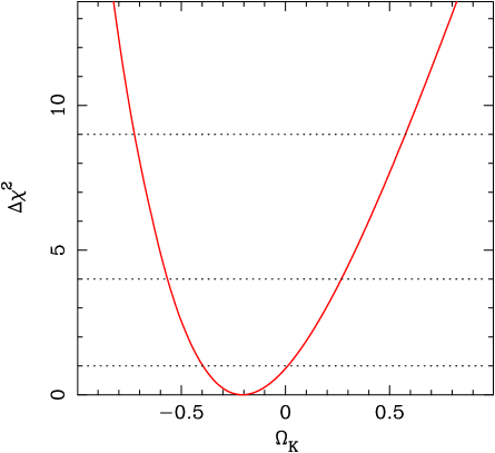
Figure 7: The marginalized constraints on $\Omega_{\rm K}$ ($=1-\Omega_{\rm m}-\Omega_{\Lambda}$) obtained from the Chandra $f_{\rm gas}$ data using the standard priors on $\Omega_{\rm b}h^{2}$ and $h$. The dotted lines mark the formal 1, 2 and 3$\sigma$ limits (see text for details).

For the $\Lambda$CDM cosmology, we have examined a grid of cosmological models covering the plane $0.0<\Omega_{\rm m}<1.0$ and $0.0<\Omega_{\Lambda}<2.0$. The joint 68.3, 95.4 and 99.7 per cent confidence contours (corresponding to $\Delta\chi^{2}$ values of 2.30, 6.17 and 11.8, respectively) obtained from the Chandra $f_{\rm gas}$ data, including standard priors on $\Omega_{\rm b}h^{2}$ (Kirkman et al. 2003) and $h$ (Freedman et al. 2001) are shown in Fig. 4. The best-fit parameters and marginalized 68 per cent confidence limits obtained using the standard priors are $\Omega_{\rm m}=0.245^{+0.040}_{-0.037}$ and $\Omega_{\Lambda}=0.96^{+0.19}_{-0.22}$, with $\chi^{2}=24.5$ for 24 degrees of freedom. The $\chi^{2}$ value indicates that the model provides an acceptable description of the data.

Fig. 5 shows the marginalized constraints on $\Omega_{\Lambda}$ obtained using both the standard and weak priors on $\Omega_{\rm b}h^{2}$ and $h$. We see that even using the weak priors ($\Omega_{\rm b}h^{2}=0.0214\pm 0.0060$, $h=0.72\pm 0.24$), the $f_{\rm gas}$ data still provide a clear detection of the effects of $\Omega_{\Lambda}$ at $>3\sigma$ significance ($\Omega_{\Lambda}=0.94^{+0.21}_{-0.23}$). A Monte Carlo analysis of the data indicates that $\Omega_{\Lambda}\leq 0$ is ruled out at $>99.9$ per cent confidence.

Fig. 4 also shows a comparison with independent constraints obtained from the CMB data using only a weak uniform prior on $h$ ($0.3<h<1.0$), and from Type 1a supernovae studies (Tonry et al. 2003). The agreement between the $f_{\rm gas}$ and CMB constraints in particular is reassuring and motivates the combined analysis of these data sets, discussed below.

Fig. 6 shows the constraints on $\Omega_{\rm m}$ and $\Omega_{\Lambda}$ obtained from the analysis of the combined $f_{\rm gas}$+CMB data set. No priors, other than the constraint $b=0.824\pm 0.089$ are assumed. We see that the $f_{\rm gas}$+CMB data set provides a remarkably tight constraint in the $\Omega_{\rm m}$,$\Omega_{\Lambda}$ plane, with best fit values and marginalized 68 per cent confidence limits of $\Omega_{\rm m}=0.28^{+0.05}_{-0.04}$ and $\Omega_{\Lambda}=0.73^{+0.04}_{-0.03}$.

Fig. 7 shows the marginalized constraints on $\Omega_{\rm K}$ ($=1-\Omega_{\rm m}-\Omega_{\Lambda}$) from the $f_{\rm gas}$ data using the standard priors on $\Omega_{\rm b}h^{2}$ and $h$. The best fit result of $\Omega_{\rm K}=-0.2\pm 0.2$ (68 per cent confidence limits) is consistent with the much tighter constraint of $\Omega_{\rm K}=-0.01\pm 0.02$ obtained from the combined $f_{\rm gas}$+CMB data set. (The CMB data alone give $\Omega_{\rm K}=-0.03^{+0.04}_{-0.06}$ using only a wide uniform prior on the Hubble constant).

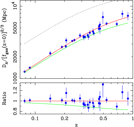
Figure 8: (Upper panel) The function $d_{\rm A}^{\rm mod}(z)/[f_{\rm gas}^{\rm mod}(z=0)]^{2/3}$ for the best-fitting $\Lambda$CDM cosmology (dark curve). Also shown are the curves obtained keeping all parameters fixed at their best-fit values but setting $\Omega_{\Lambda}=0$ (grey curve), and setting $\Omega_{\Lambda}=0$, $\Omega_{\rm m}=1$ (dotted curve). (Lower panel) The ratios with respect to the best-fitting $\Lambda$CDM model.

Finally, Fig. 8 shows an alternative way to visualize the effects of dark energy on the distances to the clusters. The model function shown in the figure is $d_{\rm A}^{\rm mod}(z)/f_{\rm gas}^{\rm mod}(z=0)^{2/3}$ and the data points $d_{\rm A}^{\rm SCDM}(z)/f_{\rm gas}^{\rm obs}(z)^{2/3}$. The use of this function removes all dependence on the reference cosmology in the figure. The dark curve in Fig. 8 shows the results for the best-fitting $\Lambda$CDM cosmology. Also shown are the curves obtained keeping the parameters fixed at their best-fit values, but setting $\Omega_{\Lambda}=0$ (grey curve; this shows the effects of the dark energy component), and setting $\Omega_{\Lambda}=0$, $\Omega_{\rm m}=1$ (dotted curve). The model including the dark energy component provides the best description of the data over the full redshift range. The $\Omega_{\Lambda}=0$, $\Omega_{\rm m}=1$ model provides a poor fit, and would require $H_{0}\sim 20$$\hbox{${\rm\thinspace km}{\rm\thinspace s}^{-1}\,$}{\rm\thinspace Mpc}^{-1}$ to approximately match the observed normalization (given the standard set of priors).

4.2 Extended XCDM models

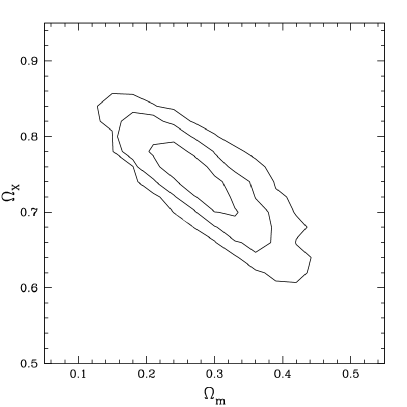
Figure 9: The 68.3, 95.4 and 99.7 per cent confidence constraints in the $\Omega_{\rm m},\Omega_{\rm X}$ plane obtained from the analysis of the combined $f_{\rm gas}$+CMB data set. We obtained marginalized 68 per cent confidence limits of $\Omega_{\rm m}=0.26^{+0.06}_{-0.04}$ and $\Omega_{\rm X}=0.75\pm 0.04$. The results are similar to those obtained for the $\Lambda$CDM models in Fig. 6.

Fig. 9 shows the 68.3, 95.4 and 99.7 per cent confidence constraints in the $\Omega_{\rm m},\Omega_{\rm X}$ plane for the extended XCDM models from the analysis of the combined $f_{\rm gas}$+CMB data set. We obtain best fitting values and marginalized 68 per cent confidence limits of $\Omega_{\rm X}=0.75\pm 0.04$ and $\Omega_{\rm m}=0.26^{+0.06}_{-0.04}$. The constraints on the mean matter and dark energy densities for the extended XCDM models are similar to those obtained for the $\Lambda$CDM cosmology. The curvature is measured to be $\Omega_{\rm K}=-0.02\pm 0.02$.

     

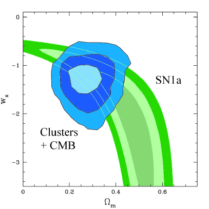
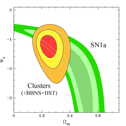
Figure 10: The 68.3, 95.4 and 99.7 per cent confidence constraints in the $\Omega_{\rm m}$,$w_{\rm x}$ plane from the analysis of (a: left panel) the combined $f_{\rm gas}$+CMB data, with $\Omega_{\rm K}$ free. Also shown, for comparison purposes, are the results obtained from the analysis of Type 1a supernovae data by Tonry et al. (2003) assuming a flat geometry. (b: right panel) The results obtained from the Chandra $f_{\rm gas}$ data alone, assuming standard priors on $\Omega_{\rm b}h^{2}$ and $h$ and a flat geometry, together with the supernovae constraints.

     

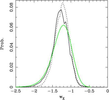
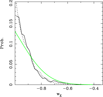
Figure 11: (a: left panel) The marginalized constraints on the equation of state parameter, $w_{\rm X}$, obtained from the $f_{\rm gas}$+CMB data with $\Omega_{\rm K}$ free (dark solid curve), $f_{\rm gas}$+CMB data assuming a flat geometry (dotted curve) and $f_{\rm gas}$ data alone assuming a flat geometry and standard priors on $\Omega_{\rm b}h^{2}$ and $h$ (grey curve). (b) As for (a) but imposing the prior constraint $w_{\rm X}>-1$.

Fig. 10(a) shows the constraints in the $\Omega_{\rm m},w_{\rm X}$ plane obtained from from the same data. Also shown, for comparison purposes, are the results from Type 1a supernovae studies (Tonry et al. 2003). Fig. 10(b) shows the results obtained from the $f_{\rm gas}$ data alone, assuming a flat geometry and the standard priors on $\Omega_{\rm b}h^{2}$ and $h$. The results are in excellent agreement with those obtained from the $f_{\rm gas}$+CMB data set. We again note the ability of the $f_{\rm gas}$ data, used in combination with the CMB data or standard priors, to break important degeneracies between parameters.

Fig. 11(a) shows the marginalized constraints on $w_{\rm X}$ for the extended XCDM models. For the $f_{\rm gas}$+CMB data with $\Omega_{\rm K}$ free we find $w_{\rm X}=-1.26^{+0.24}_{-0.24}$. Under the assumption of a flat geometry, the same $f_{\rm gas}$+CMB data data give $w_{\rm X}=-1.22^{+0.20}_{-0.22}$. For a flat geometry, the $f_{\rm gas}$ data and standard priors on $\Omega_{\rm b}h^{2}$ and $h$ give $w_{\rm X}=-1.20^{+0.24}_{-0.28}$. Note that for a flat geometry, the supernovae data alone give $w_{\rm X}=-2.2^{+0.8}_{-1.1}$ (68 per cent confidence limits).

Fig. 11(b) shows the marginalized constraints on $w_{\rm X}$ obtained from XCDM models when we apply the prior constraint $w_{\rm X}>-1$. Under this assumption, the $f_{\rm gas}$+CMB data with $\Omega_{\rm K}$ free give a 95.4 per cent confidence constraint of $w_{\rm X}<-0.69$. If we assume flatness, the same data require $w_{\rm X}<-0.75$. For a flat geometry and standard priors on $\Omega_{\rm b}h^{2}$ and $h$, the $f_{\rm gas}$ data alone give $w_{\rm X}<-0.69$. These constraints are similar to those obtained by Tonry et al. (2003; $w_{\rm X}<-0.73$) from supernovae data using a prior on $\Omega_{\rm m}$ from the 2dF Galaxy Redshift Survey ($\Omega_{\rm m}h=0.20\pm 0.03$; Percival et al. 2001) and assuming a flat geometry. Our results on $w_{\rm X}$ are also consistent with (and comparable to) those reported by the WMAP team (Spergel et al. 2003).

Finally, we note that our results for the extended XCDM cosmology imply that the mean matter and dark energy densities become equal at a redshift $z=(\Omega_{\rm m}/\Omega_{\rm X})^{1/3w_{\rm X}}-1=0.30\pm 0.09$, and that the Universe moves from a decelerating to an accelerating phase at $z=[-(1+3w_{\rm X})\Omega_{\rm X}/\Omega_{\rm m}]^{-1/3w_{\rm X}}-1=0.70\pm 0.11$ (68 per cent confidence limits).

5 Discussion

Our results provide the first clear confirmation of type Ia supernovae results in terms of detecting the effects of dark energy on distance measurements to a separate, well-defined source population. Our results cover the redshift range where the expansion of the Universe moves from a decelerating to an accelerating phase. The significance of our detection of dark energy is $>3\sigma$ ($>99.9$ per cent significance from Monte Carlo simulations) for the standard $\Lambda$CDM model with $\Omega_{\rm K}$ free, using only weak priors on $\Omega_{\rm b}h^{2}$ and $h$. This accuracy is comparable to that obtained from current supernovae work (Tonry et al. 2003; see also Riess et al. 2004).

It is interesting to note that our preferred value for $w_{\rm X}$ in the extended XCDM models is slightly less than -1, which allows the possibility that the dark energy density is increasing with time. Such a scenario is also mildly favoured by recent Type 1a supernovae studies (Tonry et al. 2003; Riess et al. 2004). We stress, however, that the Chandra results remain consistent with $\Lambda$CDM ($w_{\rm X}=-1$).

A major benefit of our technique is that the application of standard priors on $\Omega_{\rm b}h^{2}$ and $H_{0}$, or the combination with CMB data, also leads to tight constraints on $\Omega_{\rm m}$, thereby allowing important degeneracies between parameters to be broken. For a $\Lambda$CDM cosmology ($\Omega_{\rm K}$ free), we find $\Omega_{\rm m}=0.245^{+0.040}_{-0.037}$ using standard priors on $\Omega_{\rm b}h^{2}$ and $h$, or $\Omega_{\rm m}=0.28^{+0.05}_{-0.04}$ when the $f_{\rm gas}$ and CMB data are combined. These constraints are comparable to those obtained from the combination of current CMB data with a variety of other data sets and priors (e.g. Spergel et al. 2003). We note that the lower value of $\Omega_{\rm m}$ obtained in this work with respect to ASF02 is primarily due to the inclusion of the bias factor $b$ in the present study, together with changes in the prior on $\Omega_{\rm b}h^{2}$. The (slightly) larger error bars on $\Omega_{\rm m}$ are due to the inclusion of the 10 per cent systematic uncertainty in the normalization of the $f_{\rm gas}$ curve (via $b$), which is motivated by residual uncertainties in the calibration of the Chandra detectors. It may be that this 10 per cent allowance overestimates the systematics errors. If it were not included, the constraint on $\Omega_{\rm m}$ for the $\Lambda$CDM cosmology from the $f_{\rm gas}$ data using standard priors on $\Omega_{\rm b}h^{2}$ and $h$ would become $\Omega_{\rm m}=0.246^{+0.033}_{-0.029}$. Recall that the constraint on $\Omega_{\rm m}$ arises primarily from the normalization of the $f_{\rm gas}(z)$ curve and so is affected by the 10 per cent systematic uncertainty, whereas the constraint on $\Omega_{\rm X}$ is determined by the shape of the curve and is so largely independent of the uncertainties in $\Omega_{\rm b}h^{2}$, $h$ and $b$.

The evidence for dark energy from the Chandra data is robust against uncertainties in the bias factor, $b$. The results depend primarily upon the shape of the $f_{\rm gas}(z)$ curve and so doubling the overall uncertainty in $b$ to 20 per cent has little effect. Only redshift evolution in $b$ can change the results on dark energy. However, to remove the evidence for dark energy (i.e. measure $OX=0$) we would require $b$ to decrease with increasing redshift by $>30$ per cent over the interval $0<z<1$. This change in $b$ is much larger than is allowed by simulations; the study of Eke et al. (1998) indicates negligible evolution over the redshift range studied here. For illustration purposes only, we have examined the effects of including (substantial) evolution in $b$ such that $b(z)=(1-0.1z)b(0)$. This leads to only a small change in the results: $\Omega_{\Lambda}=0.72^{+0.24}_{-0.27}$ for the $\Lambda$CDM cosmology using the Chandra data and weak priors. (The detection of dark energy remains significant at the $\sim 2.5$ sigma level.) Including such evolution in $b$ also shifts the best-fit value for $w$ closer to -1 : $w=-0.98^{+0.21}_{-0.24}$ for the same data using the XCDM model.

An important aspect of the present work is that the clusters studied are regular, apparently dynamically relaxed systems. This results in a significant reduction of the scatter in the $f_{\rm gas}$ measurements with respect to studies that do not include such a selection criterion (e.g. Ettori et al. 2003). Note also that our analysis does not impose a parametric form for the X-ray gas distribution, uses a realistic parameterization for the total matter distribution, and makes full use of information on the temperature profiles in the clusters. Independent confirmation of the total masses within $r_{2500}$ is available from weak lensing studies in a number of cases, which lends support to the reliability of the $f_{\rm gas}$ measurements (see discussion in ASF02; a program to expand the weak lensing measurements to the entire sample studied here is underway.) Finally, we note that the effects of departures from spherical symmetry on the $f_{\rm gas}$ results are expected to be small ($\mathrel{\hbox to0.0pt{\lower 3.0pt\hbox{$\sim$}\hss}\raise 2.0pt\hbox{$<$}}$ a few per cent; Buote & Canizares 1996, Piffaretti, Jetzer & Schindler 2003).

An ASCII table containing the redshift and $f_{\rm gas}(z)$ data is available from the authors on request.

References

- [1] Allen S.W., Ettori S., Fabian A.C., 2001, MNRAS, 324, 877
- [2] Allen S.W., Schmidt R.W., Fabian A.C., 2002a, MNRAS, 334, L11
- [3] Allen S.W., Schmidt R.W., Fabian A.C., 2002b, MNRAS, 335, 256
- [4] Allen S.W., Schmidt R.W., Fabian A.C., Ebeling H., 2003a, MNRAS, 342, 287
- [5] Allen S.W., Schmidt R.W., Bridle, 2003b, MNRAS, 346, 593
- [6] Arnaud, K.A., 1996, in Astronomical Data Analysis Software and Systems V, eds. Jacoby G. and Barnes J., ASP Conf. Series volume 101, p17
- [7] Balucinska-Church M., McCammon D., 1992, ApJ, 400, 699
- [8] Bialek J.J., Evrard A.E., Mohr J.J., 2001, ApJ, 555, 597
- [9] Buote D.A., Tsai D.A., 1995, ApJ, 439, 29
- [10] Buote D.A., Canizares C.R., 1996, ApJ, 457, 565
- [11] Clowe D., Luppino G.A., Kaiser N., Gioia I.M., 2000, ApJ, 539, 540
- [12] David L.P., Jones C., Forman W., 1995, ApJ, 445, 578
- [13] Donahue M., Voit G.M., Scharf C.A., Gioia I.M., Mullis C.R., Hughes J.P., Stocke, J.T., 1999, ApJ, 527, 525
- [14] Ebeling H., Edge, A.C., Henry J.P., 2001, ApJ, 553, 668
- [15] Ebeling H., Jones L.R., Fairley B.W., Perlman E., Scharf C., Horner D., 2001, ApJ, 548, L23
- [16] Eke V.R., Navarro J.F., Frenk C.S., 1998, ApJ, 503, 569
- [17] Ettori S., Fabian A.C., 1999, MNRAS, 305, 834
- [18] Ettori S., Tozzi P., Rosati P., 2003, A&A, 398, 879
- [19] Evrard A.E., 1997, MNRAS, 292, 289
- [20] Fabian A.C., 1991, MNRAS, 253, L29
- [21] Freedman W. et al. , 2001, ApJ, 553, 47
- [22] Fukugita M., Hogan C.J., Peebles P.J.E., 1998, ApJ, 503, 518
- [23] Gioia I.M., Luppino G.A., 1994, ApJS, 94, 583
- [24] Hinshaw G. et al. , 2003, ApJS, 148, 135
- [25] Kaastra J.S., Mewe R., 1993, Legacy, 3, HEASARC, NASA
- [26] Kirkman D., Tytler D., Suzuki N., O’Meara J.M., Lubin D., 2003, ApJS, 149, 1
- [27] Kogut A. et al. , 2003, ApJS, 148, 161
- [28] Kuo C.L. et al. 2004, ApJ, 600, 32
- [29] Lewis A., Bridle S., 2002, Phys. Rev. D, 66, 103511
- [30] Lewis A., Challinor A., Lasenby A., 2000, ApJ, 538, 473
- [31] Liedhal D.A., Osterheld A.L., Goldstein W.H., 1995, ApJ, 438, L115
- [32] Lin Y.-T., Mohr J.J., Stanford S.S., 2003, ApJ, 591, 749
- [33] Maughan B.J., Jones L.R., Ebeling H., Scharf C., 2004, MNRAS, in press (astro-ph/0403521)
- [34] Mohr J.J., Mathiesen B., Evrard A.E., 1999, ApJ, 517, 627
- [35] Navarro J.F., Frenk C.S., White S.D.M., 1997,ApJ, 490, 493
- [36] Pearson T.J. et al. 2003, ApJ, 591, 556
- [37] Peebles P.J.E., Ratra B., 2003, Rev. Mod. Phys., 75, 559
- [38] Pen U., 1997, NewA, 2, 309
- [39] Percival W.J. et al. , 2002, MNRAS, 337, 1068
- [40] Piffaretti R., Jetzer P., Schindler S., 2003, A&A, 398, 41
- [41] Riess A.G., 2004, ApJ, in press (astro-ph/0402512)
- [42] Roussel H., Sadat R., Blanchard A., 2000, A&A, 361, 429
- [43] Sanderson A.J.R., Ponman T.J., 2003, 345, 1241
- [44] Sasaki S., 1996, PASJ, 48, L119
- [45] Schmidt R.W., Allen S.W., Fabian A.C., 2001, MNRAS, 327, 1057
- [46] Seljak U., Zaldarriaga M., 1996, ApJ, 469, 437
- [47] Spergel D.N. et al. 2003, ApJS, 148, 175
- [48] Tonry J.L. et al. , 2003, ApJ, 594, 1
- [49] Verde L. et al. , 2003, ApJS, 148, 195
- [50] White D.A., Fabian A.C., 1995, MNRAS, 273, 72
- [51] White D.A., Jones C., Forman W., 1997, MNRAS, 292, 419
- [52] White S.D.M., Frenk C.S., 1991, ApJ, 379, 52
- [53] White S.D.M., Navarro J.F., Evrard A.E., Frenk C.S., 1993, Nature, 366, 429.