The Mass Budget of Merging Quasars

Abstract

Two spectacular results emerging from recent studies of nearby dead quasars and distant active quasars are (i) the existence of tight relations between the masses of black holes (BHs) and the properties of their host galaxies (spheroid luminosity or velocity dispersion, galaxy mass), and (ii) a consistency between the local mass density in BHs and that expected by summing up the light received from distant active quasars. These results are partly shaped by successive galactic mergers and BH coalescences, since mergers redistribute the population of BHs in galaxies and BH binary coalescences reduce the mass density in BHs through losses to gravitational waves. Here, we isolate and quantify these effects by following the cosmological merger history of a population of massive BHs representing the quasar population between $z=3$ and $z=0$. Our results suggest that the relation between BH mass and host galaxy properties, and inferences on the global efficiency of BH accretion during active quasar phases, could be influenced by the cumulative effect of repeated mergers.

1 Introduction

In the past five years, our knowledge of dead and active quasars has improved considerably. For the most part, this is the result of detailed dynamical studies of nearby galactic nuclei (for dead quasars) and of several ambitious cosmological surveys (for active quasars). The progress is so significant that it is now possible to relate, in a satisfactory manner, the amount of light received from distant active quasars to the amount of mass locked into nearby dead quasars.

It has long been suspected that nearby galactic nuclei should host massive BHs (see Kormendy & Richstone 1995 for a review) but it is only recently that the evidence from detailed dynamical studies has become compelling. BHs appear to be present in the nuclei of almost all nearby luminous galaxies (Magorrian et al. 1998), and their masses correlate well with the velocity dispersion of the host galaxy’s spheroidal component (Ferrarese & Merritt 2000; Gebhardt et al. 2000; Tremaine et al. 2002; see also Haering & Rix 2004) and the galaxy’s total mass (Ferrarese 2002). A number of scenarios have been put forward to explain the origin of these relations between BH mass and host galaxy properties. They invoke a variety of physical processes, from radiative and/or mechanical feedback acting during BH formation (Silk & Rees 1998; Haehnelt, Natarajan & Rees 1998; Adams, Graff & Richstone 2001; King 2003; Wyithe & Loeb 2003b; Di Matteo et al. 2003) to dynamical processes operating in the BH environment (Ostriker 2000; Zhao, Haehnelt & Rees 2002; Merritt & Poon 2004; Miralda-Escude & Kollmeier 2004; Sellwood & Moore 1999; Shen & Sellwood 2003).

Well before the case for a local population of massive BHs was made, it had been proposed that dead quasars, the remnants of past active quasar phases, should be present in today’s galactic nuclei, and that the amount of mass locked into these BHs should be directly related to the amount of light released by distant active quasars (Lynden-Bell 1969; Soltan 1982; Rees 1990). By combining recent characterizations of the local population of massive BHs with high-quality data on nearby galaxies and distant active quasars from modern cosmological surveys (2dF: Boyle et al. 2000; SDSS: Stoughton et al. 2002), it is now possible to confirm the link between active and dead quasars with surprising accuracy.

Yu & Tremaine (2002) find a mass density $\rho_{\rm BH}\simeq 2.5\times 10^{5}$ M_⊙ Mpc^-3 for the local population of massive BHs (see also Aller & Richstone 2002). On the other hand, assuming a mass-to-light conversion efficiency $\epsilon=0.1$ for BH accretion, they also infer a mass density $\rho_{\rm BH}\simeq 2.1\times 10^{5}$ M_⊙ Mpc^-3 from the integrated light of optically-bright quasars (see also Chokshi & Turner 1992). The consistency between these two values is remarkable and it provides an effective measure of the BH accretion efficiency during (optically-bright) active quasar phases. It appears, however, that some of the light from active quasars may have been missed by optical surveys (probably because of dust obscuration), since several authors have inferred values of $\rho_{\rm BH}$ from X-ray data that exceed substantially the corresponding value for optical data (Fabian & Iwasawa 1999; Barger et al. 2001; Elvis, Risaliti & Zamorani 2002). Requiring consistency with the local value of $\rho_{\rm BH}$ then points toward a larger efficiency for BH accretion, $\epsilon\;\hbox to0.0pt{\lower 2.5pt\hbox{$\sim$}\hss}\raise 1.5pt\hbox{$>$}\;0.15$–$0.2$. As the radiative efficiency can increase for gas accreting onto spinning BHs, this may indicate that massive BHs associated with luminous quasars are spinning rapidly.

These impressive developments have focused on the “brighter side” of quasar evolution, the one that is most easily accessible to astronomers through various electromagnetic signatures of accretion onto massive BHs. Our main interest here is the “darker side” of quasar evolution, which is (currently) not easily accessible to astronomers, but could in principle be equally important in shaping the properties of the quasar population. It is a generic prediction of hierarchical CDM cosmologies that galaxies merge to grow larger and more massive with cosmic times and, as a result, the massive BHs that they harbor are expected to coalesce. BH coalescences should be observable in the future through the detection of gravitational waves accompanying these events. Studying this darker side of quasar evolution is in fact one of the main motivations behind efforts to build the Laser Interferometer Space Antenna (LISA), and several studies have already emphasized how valuable the information provided by LISA on the population of distant quasars would be (Haehnelt 1994; 2003; Menou, Haiman & Narayanan 2001; Hughes 2002; Menou 2003; Sesana et al. 2004; Islam, Taylor and Silk 2004; Wyithe & Loeb 2003a).

Here, we wish to investigate the consequences that galactic mergers and BH coalescences may have on the cosmological evolution of quasars. Specifically, we focus on two important ways in which mergers can potentially affect recent results on the populations of dead and active quasars. First, in each BH binary coalescence, a finite amount of energy is lost to gravitational waves. This translates into an effective mass loss for the remnant BH, which ends up with a mass smaller than the initial mass of its two progenitors. Although this mass loss can be as small as $\sim 6\%$ of the lowest mass progenitor, according to general relativity (see §2.3), it can also be significantly larger. Most importantly in a cosmological context, the effect is cumulative, since each individual BH experiences mergers repeatedly over time. Second, successive galactic mergers effectively redistribute the population of massive BHs in galaxies, thus changing its overall properties. For example, it is unclear whether the characteristics of a high-redshift quasar population initially similar to those of nearby dead quasars would be conserved or modified by successive cosmological mergers (see, e.g., Ciotti & van Albada 2001; Haehnelt 2003; Koushiappas, Bullock & Dekel 2004).

In the present work, we isolate and quantify these two effects by following the cosmological merger history of a plausible population of quasars. We describe our methodology in detail in §2 and discuss our results in §3.

2 Models

2.1 General Characteristics

To follow the cosmological merger history of a population of quasars, we must first describe how the galaxies hosting them evolve with cosmic times. We do this by using Monte–Carlo simulations of “merger trees” that describe the merger history of dark matter halos (and associated galaxies) in the standard $\Lambda$CDM cosmology ($\Omega_{0}=0.3$, $\Omega_{b}=0.04$, $\Omega_{\Lambda}=0.7$, $h_{100}=0.65$). The specific merger tree we are using, and a number of additional model assumptions, are described in detail in Menou et al. (2001). The range of halo masses considered (e.g. $\sim 10^{9}$–$10^{13}$ M_⊙ at $z=0$, for a fixed comoving volume of $\sim 1.7\times 10^{4}$ Mpc³) guarantees that one-to-one associations between dark matter halos and galaxies are reasonably accurate (Menou et al. 2001). One of the main model assumptions is that only galaxies with a virial temperature in excess of $10^{4}$ K are able to host a BH because they are the only ones in which baryon cooling is efficient enough to allow BH formation (see, e.g., Loeb & Barkana 2001 and Haiman & Quataert 2004 for reviews). By construction, the merger tree describes only “interesting” halos with virial masses in excess of a temperature-equivalent of $10^{4}$ K.

The complex and uncertain physics of baryon cooling and galaxy formation is not described by our models. As a result, no attempt is made to separate from the rest a bulge-less galactic population, which may or may not be able to harbor massive BHs according to recent studies (Gebhardt et al. 2001; Merritt et al. 2001, but see Salucci et al. 2000). Accounting for several different galactic types in our simulations would further complicate their interpretation and we have chosen, for simplicity, to assume that every halo described by the tree is a possible host for a massive BH.

Currently, observational constraints on the presence of massive BHs in low-mass galaxies are very scarce and various arguments have been put forward to suggest that these galaxies may not be able to form, or perhaps retain, massive BHs (e.g. Haiman, Madau & Loeb 1999; Ferrarese 2002; Haiman, Quataert & Bower 2004; Haehnelt et al. 1998; Silk & Rees 1998; Favata, Hughes & Holz 2004; Merritt et al. 2004; Madau & Quataert 2004; Bromley, Somerville & Fabian 2004; but see also Barth et al. 2004). In order to maximize the cumulative effects of successive BH mergers, we assume by default that a massive BH is present in all the galaxies described by the merger tree. For the sake of generality, however, we will also investigate alternative scenarios in which BHs preferentially populate massive galaxies, at least initially.

A realistic model for the cosmological evolution of a population of quasars should describe simultaneously the action of mergers and accretion on the population of massive BHs. Such models exist already (e.g. Kauffmann & Haehnelt 2000; Volonteri, Haardt & Madau 2003) and their focus generally is on reproducing a number of observational constraints available for the bright side of quasar evolution. However, these studies have not isolated the contribution due to mergers and have not included gravitational wave losses when computing the evolution of BH masses. Our goal here is not to construct a realistic evolution scenario for quasars, but precisely to isolate and quantify the effects that mergers and coalescences may have on the quasar population.

Recent quasar evolutionary studies indicate that massive BHs acquired most of their accreted mass over a wide range of redshifts, approximately $90\%$ of it from $z\simeq 3$ to $z\simeq 0$ (see, e.g., Fig. 1 of Yu & Tremaine 2002, or Fig. 8 of Marconi et al. 2004). Consequently, both mergers and accretion will act to shape the main properties of the quasar population over this range of redshifts. In our models, we take no account of accretion, and instead assume that the population of massive BHs present at $z=3$ evolves from $z=3$ to $z=0$ only through a hierarchy of mergers. We emphasize that this assumption is not intended to yield a realistic description of the observed quasar population. Rather, the motivation behind this assumption is to provide a robust clarification of the role of mergers alone.

Making this assumption still leaves the detailed characteristics of the quasar population in place at $z=3$ completely open, in the sense that the BH mass can be distributed in host galaxies in many different ways. The results of Shields et al. (2003) indicate, however, that the properties of massive BHs associated with luminous quasars at $z\simeq 3$ are consistent with the properties of dead quasars studied locally. Based on this result, we have chosen to investigate the effects of mergers on a population of quasars with characteristics similar to those of local dead quasars. In the next subsection, we describe in further detail how BH masses were chosen with respect to the mass of host galaxies in our models.

2.2 Black Hole Masses

We consider two different, albeit related models for the initial distribution of BH masses in galaxies at $z=3$. Our main motivation for exploring two mass models is the possibility that our results (at $z=0$) are sensitive to the exact characteristics of the BH population assumed to be present at $z=3$. In the first class of models (“T models”), BH masses are chosen according to the relation established by Tremaine et al. (2002),

$$M_{\rm bh}=\left(1.35\pm 0.2\right)\times 10^{8}M_{\odot}\left(\frac{\sigma_{e}}{200~{}{\rm km~{}s^{-1}}}\right)^{4.02\pm 0.32},$$ (1)

where $\sigma_{e}$ is the stellar velocity dispersion of the spheroidal component at the half-light (effective) radius. It is related to $\sigma_{\rm dm}$, the halo velocity dispersion, via the relation $\sigma_{e}=\sigma_{\rm dm}/\sqrt{3/2}$, which is derived from the Jeans equation for isotropic, spherical systems, assuming an isothermal density profile ($\rho\propto r^{-2}$) for the dark matter and a typical DeVaucouleurs density profile ($\rho\propto r^{-3}$) for the stellar spheroidal component. The halo velocity dispersion is obtained from the virial theorem and the assumption that halos have a universal density,

$$\sigma_{\rm dm}=17\left(\frac{M_{\rm halo}}{10^{8}M_{\odot}h}\right)^{1/3}\left(\frac{\delta_{c}}{200}\right)^{1/6}\left(\frac{1+z}{10}\right)^{1/2},$$ (2)

where $\delta_{c}(z)$ is the cosmological density contrast at collapse. This is the exact same prescription as the one adopted in Menou (2003).

In the second class of models (“FWL models”), BH masses are chosen according to the relation established locally by Ferrarese (2002; with a different $\sigma_{e}$–$\sigma_{\rm dm}$ relation than above) and extended to higher redshifts by Wyithe & Loeb (2004),

$$M_{\rm bh}=10^{9}M_{\odot}\left(\frac{M_{\rm halo}}{1.5\times 10^{12}M_{\odot}}\right)^{5/3}\left(\frac{1+z}{7}\right)^{5/2}.$$ (3)

A similar prescription (with a somewhat smaller normalization) has been adopted by Haiman, Quataert & Bower (2004) for their predictions on high-redshift radio-loud quasars.

The two prescriptions (T and FWL) have a similar dependence on redshift ($(1+z)^{2}$ vs. $(1+z)^{5/2}$) but different normalizations and power-law scalings with $M_{\rm halo}$ ($\sim 4/3$ for T vs. $5/3$ for FWL). Another difference is the initial presence of scatter in the T relation (see equation [1]), which is included in our T models but is absent from FWL models.

2.3 Gravitational Wave Losses

When two galaxies hosting massive BHs merge, several processes act successively to bring the BHs closer to the galactic remnant’s center, have them form a bound binary and ultimately make them coalesce (Begelman, Blandford & Rees 1980). The first such process is dynamical friction, which is thought to be rather efficient initially (but see discussion in §2.4). When the separation between the two BHs reduces to parsec scales typically, other mechanisms must be invoked, however (e.g. repeated stellar ejections, gaseous interaction). These mechanisms have been investigated in detail (see, e.g., Milosavljevic & Merritt 2003; Blaes, Lee & Socrates 2002; Gould & Rix 2000; Armitage & Natarajan 2002 for recent results) but the efficiency with which they act to shrink the orbit of a massive BH binary is still much debated. Ultimately, at sub-parsec separations, emission of gravitational waves takes over as the leading mechanism for the loss of energy and angular momentum from the binary, until the two BHs coalesce.

As we have already emphasized, our main interest here is in isolating the effects of mergers on a quasar population. For this reason, we will neglect complexities related to the various processes we have just mentioned and assume by default in our models that two BHs coalesce efficiently right after their host galaxies merge. This assumption simplifies the models greatly and it is consistent with our effort to quantify the effects that many successive mergers may have on a quasar population.

During their final shrinking phases, massive BH binaries will therefore lose energy in the form of gravitational waves, but the total amount of mass-energy lost after coalescence is complete is not well known. A first source of uncertainty arises from general relativistic calculations, because of the non-linear character of the strong-field interaction between the two BHs. A second source of uncertainty comes from the necessity of knowing the masses and the spins of the two BHs involved, as well as the orbital geometry, to make accurate predictions. While the masses of BHs in nearby dead quasars are known with some accuracy, masses of BHs in more distant quasars are not so well known and essentially no information is available on BH spins. In the context of quasar evolution, where both mergers and accretion contribute to the coupled mass and spin evolution of BHs (in a way which has yet to be elucidated; see, e.g., Gammie, Shapiro & McKinney 2004 and Hughes & Blandford 2003 for recent discussions), it is not possible to provide an accurate description of the spin evolution of quasar BHs.

The coalescence of two BHs is often decomposed in three successive phases (see, e.g., Hughes 2002 and references therein): the slow inspiral phase (when the two BHs spiral in quasi-adiabatically), the dynamical plunge phase (when the two BHs plunge towards each other and their horizons merge) and the final ringdown phase (when the merger remnant relaxes to a stationary Kerr BH solution). Emission of gravitational waves during the plunge phase is not well understood because it is not well approximated by perturbative methods. Small losses during this phase are generally expected because of its short duration. Significant progress with numerical simulations has been made in recent years but the problem has not been addressed yet in full generality (see Baumgarte & Shapiro 2003 for a review). The emission of gravitational waves during the ringdown phase is also subject to uncertainties, since its initial condition is the unknown outcome of the plunge phase, but it is also expected to contribute a relatively small amount to the total energy lost during coalescence (Khanna et al. 1999).

Emission of gravitational waves during the inspiral phase is comparatively much better understood. Losses are calculated by identifying the location of the Innermost Stable Circular Orbit (ISCO), which corresponds to the minimum separation that the two massive BHs are able to reach via slow inspiral before plunge. For example, for very small mass ratios (approaching the test particle case), it is well known that the binary loses the equivalent of $\sim 6\%$ of the rest mass of the less massive BH if the more massive one is non-rotating, and $\sim 42\%$ of the rest mass of the less massive BH if the more massive one is maximally-rotating (from arguments similar to those yielding the radiative efficiency of gas accretion onto BHs, see, e.g. Shapiro & Teukolsky 1983). Losses during the subsequent plunge and ringdown phases would have to be added to these figures.

Independently of the details of the merger process, the BH area theorem of general relativity also puts strict limits on the total amount of energy lost to gravitational waves when two BHs coalesce. Although it is likely that these bounds largely overestimate the actual losses in astrophysical coalescences, they are still useful in providing firm upper limits on the cumulative effects of mergers on a quasar population.

In view of all the above uncertainties, we explore five simple prescriptions for gravitational wave losses in our models. In a given evolutionary model for the quasar population, the same prescription is adopted for all BH binary coalescences. Let us denote by $M_{1}$ the mass of the most massive BH involved and $M_{2}$ that of the lowest mass BH ($M_{1}=M_{2}$ never occurs exactly in our models, even if sometimes $M_{1}\simeq M_{2}$).

1. In models with suffix “0,” losses to gravitational waves are neglected and the masses $M_{1}$ and $M_{2}$ are simply added up during coalescences. The interest of this model is that it allows us to isolate the effects of galactic mergers on the quasar population, independently of gravitational wave losses.
   

2. In models with suffix “6,” losses to gravitational waves are taken to be $6\%$ of $M_{2}$. This corresponds to a situation in which the largest mass BH ($M_{1}$) is non-rotating (Schwarzschild), the mass ratio is assumed to be very small ($M_{2}/M_{1}\ll 1$) and losses during the plunge and ringdown phases are neglected.
   

3. In models with suffix “42,” losses to gravitational waves are taken to be $42\%$ of $M_{2}$. This corresponds to a situation in which the largest mass BH ($M_{1}$) is maximally rotating (max-Kerr), the mass ratio is assumed to be very small ($M_{2}/M_{1}\ll 1$) and losses during the plunge and ringdown phases are neglected.
   

4. In models with suffix “adS,” the maximum losses allowed by the BH area theorem for the coalescence of two Schwarzschild BHs resulting in a Schwarzschild BH are adopted. The corresponding mass deficit is $\Delta M=M_{1}+M_{2}-\sqrt{M_{1}^{2}+M_{2}^{2}}$, with a maximum of $29\%$ when $M_{1}=M_{2}$ (e.g., Shapiro & Teukolsky 1983).
   

5. In models with suffix “adK,” the maximum losses allowed by the BH area theorem for the coalescence of two counter-rotating max-Kerr BHs resulting in a Schwarzschild BH are adopted. The corresponding mass deficit is $\Delta M=M_{1}+M_{2}-\sqrt{(M_{1}^{2}+M_{2}^{2})/2}$, with a maximum of $50\%$ when $M_{1}=M_{2}$ (e.g., Shapiro & Teukolsky 1983).

2.4 Inefficient Dynamical Friction

By accounting for the gradual tidal evaporation of the stellar cluster initially bound to a massive BH which experiences dynamical friction in a realistic galaxy model, Yu (2002) has argued that binary BHs with mass ratios $M_{2}/M_{1}<10^{-3}$ are unable to form: the dynamical friction time for the smallest mass BH ($M_{2}$) then exceeds a Hubble time. Although this argument has been developed for local galaxies, similar conclusions may hold for galaxies at higher redshifts. It would imply that massive BH binaries with large mass ratios are unable to merge and it could thus potentially influence our study of the cumulative effects of mergers on a quasar population.

To test the influence of inefficient dynamical friction, we have also constructed models in which massive BH binaries are not allowed to coalesce unless their mass ratio is large enough.

1. In models with suffix “q3,” following Yu (2002), we assume that BH binaries coalesce only if $M_{2}/M_{1}>10^{-3}$. In galactic mergers involving BHs which do not satisfy the above constraint, the lowest mass BH ($M_{2}$) is simply ignored from the subsequent cosmological evolution. Losses to gravitational waves are also ignored for all BH coalescences, so that the effect of inefficient dynamical friction can be isolated.
   

2. In models with suffix “q2,” we assume that dynamical friction is even less efficient than above and allow BH binaries to coalesce only if $M_{2}/M_{1}>10^{-2}$.

3 Results

3.1 Forced Models

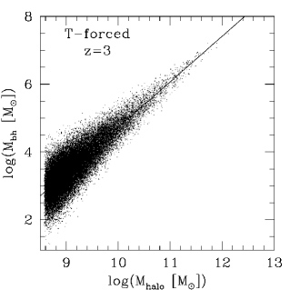
Figure 1: Initial distribution of black hole masses ($M_{\rm bh}$) and halo masses ($M_{\rm halo}$) at $z=3$ for a population of quasars following a relation adopted from Tremaine et al. (2002; T-forced at $z=3$ in the notation of Table 1). The solid line is a least-square fit to the distribution (see Table 1 for parameters).

Figure 1 shows the initial distribution of $M_{\rm bh}$–$M_{\rm halo}$ in a T-model at $z=3$. Halo masses range from $\sim 3\times 10^{8}$ M_⊙ to $\sim 10^{12}$ M_⊙ in the merger tree at this redshift and the corresponding range of BH masses is $\sim 10^{2}$ M_⊙ to $3\times 10^{7}$ M_⊙, with significant scatter for a given halo mass (from Eqs. [1] and [2]). Given the fixed comoving volume of $\sim 1.7\times 10^{4}$ Mpc³ described by the merger tree, it is possible to sum up all the BH masses in the model and deduce a mass density in BHs at $z=3$: $\rho_{\rm BH}\simeq 7.3\times 10^{4}$ M_⊙ Mpc^-3. This value is about a factor four smaller than the value measured locally, even though we have used an observationally determined relation (Eq. [1]) to populate our halos with BHs. The origin of this discrepancy lies, in fact, in the limited number of simulated halos described by the merger tree that we are using. As can be seen from Fig. 1, massive halos are scarce (e.g. only one halo in excess of $10^{12}$ M_⊙ at $z=3$). Since the BH mass function is dominated by large mass BHs, the statistical scarcity of massive halos in the tree results in a somewhat underestimated value of $\rho_{\rm BH}$. This situation does not limit the predictive power of our models, however, as long as we are careful enough to characterize how our results depend on halo masses. A similar exercise for a population of quasars following the FWL relation (Eq. [3]), instead of the T relation, at $z=3$ results in a value of $\rho_{\rm BH}\simeq 1.4\times 10^{5}$ M_⊙ Mpc^-3, only a factor of $\sim 2$ times smaller than the measured value.

In order to quantify the results of our simulations for the $M_{\rm bh}$–$M_{\rm halo}$ relation, we have found it useful to perform least-square fits to distributions such as the one shown in Fig. 1. Assuming a dependence of the form

$$\log(M_{\rm bh})=n\times\log(M_{\rm halo})+\alpha,$$ (4)

where both $M_{\rm bh}$ and $M_{\rm halo}$ are expressed in solar units, the least-square algorithm provides us with best fit values for $n$, $\alpha$ and the residual scatter, $\sigma$, around the best fit line. Often, our results show significant dependence on $M_{\rm halo}$, so we also perform least square fits restricted to masses $M_{\rm halo}>10^{11}$ M_⊙. The parameters resulting from these restricted fits are noted $n_{11}$, $\alpha_{11}$ and $\sigma_{11}$. Note that our goal in performing these fits is not to provide accurate descriptions of the $M_{\rm bh}$–$M_{\rm halo}$ distribution, but simply to provide quantitative means to compare results from different models.

30pcMODEL PROPERTIES (Mass Density and LSQ–Fit Parameters) Model $\rho_{\rm BH}$ $n_{11}$ $\alpha_{11}$ $\sigma_{11}$ $n$ $\alpha$ $\sigma$ (M_⊙ Mpc^-3) T–forced at $z=3$ $7.3\times 10^{4}$ $1.36$ $-8.90$ $0.16$ $1.35$ $-8.73$ $0.37$ FWL–forced at $z=3$ $1.4\times 10^{5}$ $1.67$ $-11.90$ $0.00$ $1.67$ $-11.90$ $0.00$ Trare–forced at $z=3$ $6.0\times 10^{4}$ $1.34$ $-8.71$ $0.14$ $1.34$ $-8.68$ $0.28$ T0 $7.3\times 10^{4}$ $1.19$ $-7.47$ $0.13$ $1.38$ $-9.62$ $0.37$ FWL0 $1.4\times 10^{5}$ $1.46$ $-10.42$ $0.19$ $1.57$ $-11.70$ $0.26$ Trare0 $6.0\times 10^{4}$ $1.30$ $-8.82$ $0.19$ $1.27$ $-8.58$ $0.31$ T6 $6.9\times 10^{4}$ $1.18$ $-7.41$ $0.14$ $1.37$ $-9.52$ $0.37$ T42 $5.0\times 10^{4}$ $1.14$ $-7.05$ $0.18$ $1.30$ $-8.85$ $0.37$ FWL42 $1.1\times 10^{5}$ $1.43$ $-10.16$ $0.25$ $1.50$ $-11.11$ $0.28$ Trare42 $4.4\times 10^{4}$ $1.22$ $-7.98$ $0.22$ $1.18$ $-7.65$ $0.32$ TadS $3.4\times 10^{4}$ $1.07$ $-6.46$ $0.24$ $1.21$ $-8.03$ $0.38$ TadK $3.8\times 10^{3}$ $-0.27$ $7.31$ $0.31$ – – – Tq3 $7.2\times 10^{4}$ $1.19$ $-7.44$ $0.13$ $1.38$ $-9.59$ $0.37$ Tq2 $7.0\times 10^{4}$ $1.18$ $-7.33$ $0.13$ $1.38$ $-9.59$ $0.37$

Table 3.1 lists the properties of most of the models we have explored in this study. In each case, the value of the BH comoving mass density, $\rho_{\rm BH}$, and the various fit parameters are given. The first group of models in Table 3.1 (first 3 lines) corresponds to models in which the quasar population was forced to follow one or the other prescription for BH masses (T-forced or FWL-forced) at $z=3$. The second group of models (last 11 lines) corresponds to “evolutionary” models in which the quasar population was forced to follow only initially one or the other prescriptions for BH masses (at $z=3$). After that, the quasar population is evolved through successive cosmological mergers according to one of the prescriptions for gravitational wave losses or BH coalescences defined in §2. For this second group of models, properties are only listed in Table 3.1 at $z=0$, after cosmological evolution is complete.

The first group of “forced” models is useful to illustrate a number of general properties and for comparison with the second group of “evolutionary” models. Least square fits to forced models, such as the one shown in Fig. 1 (T-forced at $z=3$), recover the correct value for the slope of the $M_{\rm bh}$–$M_{\rm halo}$ relation ($n$ and $n_{11}\simeq 4/3$ for T-forced models and $\simeq 5/3$ for FWL-forced models; see Table 3.1). They also show that the scatter in the distribution is dominated by small masses ($\sigma_{11}>\sigma$), as is visually suggested by Fig. 1.

3.2 Evolutionary Models

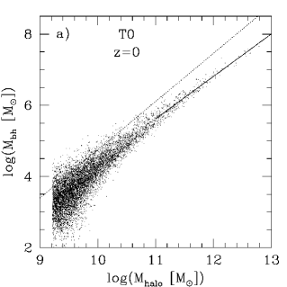
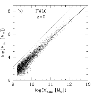
Figure 2: $M_{\rm bh}$–$M_{\rm halo}$ end distributions for populations of quasars having experienced a series of cosmological mergers from $z=3$ to $z=0$. Efficient black hole coalescence following a galactic merger is assumed and energy losses to gravitational waves are neglected. Solid lines are least-square fits to the distributions, restricted to $M_{\rm halo}>10^{11}~{}M_{\odot}$ (see Table 1 for fit parameters). Model T (a) corresponds to a population initially following a relation adopted from Tremaine et al. (2002) at $z=3$, while model FWL corresponds to a population initially following a relation adopted from Ferrarese (2002) and Wyithe & Loeb (2004). Dotted lines are least-square fits obtained for populations which are forced to follow the T or FWL relations at $z=3$. The cumulative effect of mergers is to flatten the $M_{\rm bh}$–$M_{\rm halo}$ relation, especially at large masses.

Figure 2 shows the $M_{\rm bh}$–$M_{\rm halo}$ end distributions which result when quasar populations are forced only initially to follow either the T-relation (a) or the FWL-relation (b) at $z=3$ and are subsequently left to evolve via cosmological mergers, without any mass loss to gravitational waves. In this case, the total mass locked into BHs is conserved over cosmic times and the value of $\rho_{\rm BH}$ at $z=0$ is the same as the original value at $z=3$ ($\rho_{\rm BH}\simeq 7.3\times 10^{4}$ M_⊙ Mpc^-3 for the T0 model and $\simeq 1.4\times 10^{5}$ M_⊙ Mpc^-3 for the FWL0 model; see Table 3.1).

Still, the quasar population is redistributed among galaxies of different masses through cosmological mergers and this modifies the $M_{\rm bh}$–$M_{\rm halo}$ distribution in both models. Fit parameters for the entire distribution and for the distribution restricted to $M_{\rm halo}>10^{11}$ M_⊙ are given in Table 3.1 for both models. Solid lines in Fig. 2a and 2b, which are the best fit lines to the restricted distributions, have significantly flatter slopes than the best fit lines for forced models at $z=3$ (dotted lines). This shows that the cumulative effect of mergers (without any contribution from gravitational wave losses) is to flatten the $M_{\rm bh}$–$M_{\rm halo}$ relation. The effect is clearly stronger at large masses since the slope difference is much less pronounced if one considers the entire $M_{\rm bh}$–$M_{\rm halo}$ distributions (see fit parameters in Table 3.1). This result arises because the more massive halos have experienced a larger number of mergers. Under the assumption that the two BH masses simply add together in a merger, each merger event will cause the resulting BH mass to fall below the $M_{\rm bh}$–$M_{\rm halo}$ relation.

The overall normalization of the two end distributions shown in Fig. 2, below the dotted lines, is not very meaningful. Note that the forced models at $z=3$ (dotted lines) have the exact same value of $\rho_{\rm BH}$ as the $M_{\rm bh}$–$M_{\rm halo}$ distributions at $z=0$ shown in Fig. 2a and 2b even if it is not obviously apparent (compare T0 and FWL0 with T-forced and FWL-forced at $z=3$ in Table 3.1). What is significant, however, is the difference in slope of the $M_{\rm bh}$–$M_{\rm halo}$ relation, especially at large masses, which results purely from cosmological mergers.

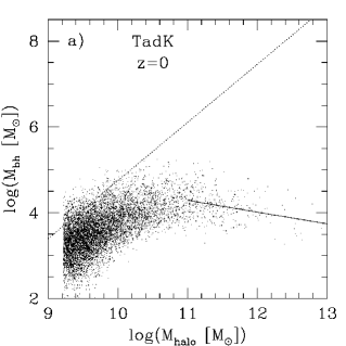
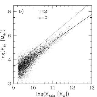
Figure 3: $M_{\rm bh}$–$M_{\rm halo}$ end distributions in (a) a model with maximal losses to gravitational waves (TadK) and (b) a model with losses to gravitational waves appropriate for a quasar population with fast–spinning black holes (T42).

Figure 3 shows the additional effects that gravitational wave losses have on the $M_{\rm bh}$–$M_{\rm halo}$ distribution. In Fig. 3a, the most extreme (and arguably unrealistic) prescription for gravitational wave losses was adopted, with dramatic consequences for the $M_{\rm bh}$–$M_{\rm halo}$ relation, especially at large masses. A least square fit is no longer satisfactory to represent the distribution and, more importantly, all the massive BHs in the model have lost most of their mass. As a result, the value of $\rho_{\rm BH}$ has dropped by more than one order of magnitude from $z=3$ to $z=0$ (compare T-forced at $z=3$ with TadK in Table 3.1). While grossly exaggerated, the TadK model is useful to highlight the consequences of gravitational wave losses. Similar conclusions hold for the TadS model, even if the effects are not as pronounced (not shown here; see Table 3.1).

Figure 3b shows the $M_{\rm bh}$–$M_{\rm halo}$ end distribution in model T42, which may be considered as more realistic for a population of quasars with systematically very fast-spinning BHs (see discussion in §2.3). The total decrease in $\rho_{\rm BH}$ at $z=0$ is $\sim 30\%$ and the flattening of the $M_{\rm bh}$–$M_{\rm halo}$ relation is more pronounced than without any gravitational wave losses (compare T42 with T0 in Table 3.1). Again, these effects clearly dominate for the largest mass BHs and halos. As before, this is simply because of the larger number of mergers experienced by more massive halos. Since mass is lost to gravitational waves in each merger, the BHs in these massive halos will accumulate a more significant decrease in their final mass at $z=0$.

Figure 4: $M_{\rm bh}$–$M_{\rm halo}$ end distributions in (a) a model without any loss to gravitational waves but a ten–times rarefied population of quasars, with black holes initially located in the most massive halos at $z=3$ (Trare0) and (b) the same model with losses to gravitational waves appropriate for a quasar population with fast–spinning black holes (Trare42).

We have already noted that quasar populations could be rarer than assumed in our standard models. Given indications that mergers preferentially influence the properties of BHs at large masses, it is important to verify whether our results still hold for a rarer population of quasars. A specific class of “rare” models that we have investigated are models in which the total number of BHs is reduced by a factor $10$ and the remaining $10\%$ are forced to systematically populate the $10\%$ most massive halos present in the tree at $z=3$. Because the mass density in BHs is dominated by large masses for the mass prescriptions we have adopted, the value of $\rho_{\rm BH}$ in these rare models is only reduced by a small fraction as compared to models with large quasar populations (compare T-forced with Trare-forced at $z=3$ in Table 3.1). Note that we have also investigated a second class of models in which an equally rare population of BHs ($10\%$) populates, this time randomly, all the halos present in the tree at $z=3$. In these models, the $M_{\rm bh}$–$M_{\rm halo}$ relation initially in place at $z=3$ is rapidly wiped out by successive cosmological mergers when the few galaxies hosting BHs experience mergers with more massive, BH-free galaxies. We therefore consider this second class of models with rare BHs as implausible.

Figure 4 shows our results for $M_{\rm bh}$–$M_{\rm halo}$ distributions in models with a rare population of quasars such that BHs are initially located in the most massive halos at $z=3$. Model Trare0 (Fig. 4a; no loss to gravitational waves) shows that one consequence of such a rare population of quasars is a noticeable reduction in the flattening effect of cosmological mergers on the $M_{\rm bh}$–$M_{\rm halo}$ relation (see also Table 3.1). Still, model Trare42 (Fig. 4b) shows that when the effects of gravitational wave losses are included, significant flattening of the $M_{\rm bh}$–$M_{\rm halo}$ relation persists. The decrease in $\rho_{\rm BH}$ due to gravitational wave losses also remains significant in models with a rare population of quasars, $\sim 27\%$ (compare Trare-forced at $z=3$ with Trare42 in Table 3.1), even if the effect is less severe because of a reduction in the total number of BH mergers in these models.

3.3 Additional Results

We have investigated a few other models in which a BH was assumed to be present in each halo; the results from these models are listed in Table 3.1. Model T6, which incorporates smaller losses to gravitational waves during BH coalescences, still shows noticeable flattening of the $M_{\rm bh}$–$M_{\rm halo}$ relation and some reduction in the value of $\rho_{\rm BH}$. Models Tq3 and Tq2, on the other hand, show that the effects of inefficient dynamical friction, which preferentially affect small mass ratios and thus small mass BHs, are not very important (compare Tq3 and Tq2 with T0 in Table 3.1).

Figure 5: (a) Evolution via successive mergers of the black hole comoving mass density, $\rho_{\rm BH}$, as a function of redshift, according to different prescriptions for gravitational wave losses (model T6: dashed line; model T42: solid; model TadS: dash-dotted; model TadK: dotted). (b) Percentage of the black hole mass density lost at $z=0$, as a function of the mass density itself (model T6: dashed; model T42: solid). An extrapolation of our results to the currently-measured value, $\rho_{\rm BH}\sim 3\times 10^{5}$ M_⊙ Mpc^-3 (vertical dotted line), suggests that losses $>30\%$ are possible.

While we have found some evidence that the magnitude of flattening of the $M_{\rm bh}$–$M_{\rm halo}$ relation due solely to cosmological mergers may be reduced for a rare and massive population of quasars, the effects due to gravitational wave losses appear to be important in all cases, especially in terms of the $\rho_{\rm BH}$ deficit. Figure 5a shows, for models T6, T42, TadS and TadK, that this deficit is related to mergers which occur over a wide range of redshifts and therefore does not strongly depend on our specific choice of $z=3$ as the initial redshift in our models (even if starting at a smaller initial redshift would obviously reduce the value of the $\rho_{\rm BH}$ deficit at $z=0$).

We have seen previously that the $\rho_{\rm BH}$ deficit due to gravitational wave losses is preferentially due to losses at large BH masses (see, e.g., Fig. 3a), because these BHs reside in larger mass halos which experience a larger number of mergers, on average. We have also already commented on the limiting size of the merger tree used, which results in a relative scarcity of very massive halos and is the reason behind the systematically small values of $\rho_{\rm BH}$ found in our models, as compared to the observationally inferred value. It is natural to wonder, then, if values for the $\rho_{\rm BH}$ deficit due to gravitational wave losses could also be underestimated in our models because of the statistical scarcity of massive halos.

We have attempted to answer this question by measuring how the $\rho_{\rm BH}$ deficit at $z=0$ depends on the range of halo masses included in the merger tree. Figure 5b shows graphically the result of this exercise and confirms our expectations. The total $\rho_{\rm BH}$ deficit accumulated at $z=0$ (expressed in $\%$ loss relative to the no-loss value) is shown for models T6 and T42, as a function of the value taken by $\rho_{\rm BH}$ as we remove an increasingly large number of the most massive halos present in the tree at $z=0$. Although this test cannot replace a full investigation with a larger tree, it does show that most of the $\rho_{\rm BH}$ deficit is related to the few most massive BHs and halos and it suggests, via an extrapolation to $\rho_{\rm BH}\sim 3\times 10^{5}$ M_⊙ Mpc^-3 (the measured value, indicated by a vertical solid line in Fig. 5b) that $\rho_{\rm BH}$ deficits $>30\%$ are expected in T42 models constructed with larger trees.

4 Discussion and Conclusion

In this study, we have isolated and quantified the effects that repeated galactic mergers and BH binary coalescences may have on a population of quasars in a cosmological context. While the characteristics of the local population of dead quasars is relatively well known, it is not the case for more distant quasars and we have therefore represented these quasars with a variety of plausible populations of massive BHs (T- and FWL-models, Trare models in Table 3.1).

Our models indicate that galactic mergers alone (excluding gravitational wave losses) influence somewhat the properties of the quasar population, by redistributing BHs in galaxies and flattening the $M_{\rm bh}$–$M_{\rm halo}$ relation. The effect appears to be small for a rare population of BHs preferentially located in massive galaxies (as may be expected, for instance, from recoil effects; Favata et al. 2004). This lends support to the idea that the high-redshift quasar population has properties which are rather similar to those of local dead quasars.

According to our models, however, losses to gravitational waves during repeated BH binary coalescences have the potential to modify substantially the characteristics of the quasar population. First, they contribute to the flattening of the $M_{\rm bh}$–$M_{\rm halo}$ relation by preferentially reducing the mass of the largest BHs, since these BHs experience a larger number of mergers. Second, losses to gravitational waves systematically reduce the BH mass density, $\rho_{\rm BH}$, over cosmic times. This potentially important cumulative effect reaches up to $30\%$ of the no–loss value of $\rho_{\rm BH}$ in our models with a population of maximally rotating BHs, and we have argued that the effect could be even stronger had we used a larger cosmological merger tree.

One must keep in mind that our models are idealized in several ways. We have neglected the growth in BH mass due to accretion. We note, for instance, that in models describing accretion, a flattening of the $M_{\rm bh}$–$M_{\rm halo}$ relation could be counter-balanced by prescribing accretion onto massive BHs in such a way as to reproduce the apparently similar relation existing between BHs and their host galaxies at $z=0$ and at $z=3$ (Shields et al. 2003). Our estimation of the effects due to gravitational wave losses is also very much simplified by adopting idealized loss prescriptions and assuming that all BH binaries coalesce efficiently with a same prescribed loss.

Still, our models suggest that the issue of losses to gravitational waves may be important for the interpretation of the quasar mass budget. A deficit in the mass budget of local dead quasars relative to that of distant active quasars has usually been interpreted as resulting from highly efficient BH accretion during active quasar phases ($\epsilon>0.1$; see §1). The results presented here indicate that part of this local mass deficit could be attributed instead to gravitational wave losses accumulated over cosmic times during repeated BH binary coalescences. In a companion study (Menou & Haiman 2004), we put more stringent limits on the role of gravitational wave losses in modifying the mass budget of merging quasars, by using more accurate loss prescriptions based on detailed general relativistic calculations.

References

- [1] F. C. Adams, D. S. Graff and D. O. Richstone, ApJ 551, L31 (2001).
- [2] M. C. Aller and D. Richstone, AJ 124, 3035 (2002).
- [3] A. J. Barger et al., AJ 122, 2177 (2001).
- [4] A. J. Barth et al., ApJ in press, astro-ph/0402110 (2004).
- [5] T. W. Baumgarte and S. L. Shapiro, Phys. Rep. 376, 41 (2003).
- [6] O. Blaes, M. H. Lee and A. Socrates, ApJ 778, 775 (2002).
- [7] M. C. Begelman, R. D. Blandford and M. J. Rees, Nature 287, 307 (1980).
- [8] B. J. Boyle, MNRAS 317, 1014 (2000).
- [9] J. M. Bromley, R. S. Somerville and A. C. Fabian, MNRAS in press, astro-ph/0311008 (2004).
- [10] A. Chokshi and E. L. Turner, MNRAS 259, 421 (1992).
- [11] L. Ciotti and T. S. van Albada, ApJ 552, L13 (2001).
- [12] T. Di Matteo et al., ApJ 593, 56 (2003).
- [13] M. Elvis, G. Risaliti and G. Zamorani, ApJ 565, L75 (2002).
- [14] A. Fabian and K. Iwasawa, MNRAS 303, 34 (1999).
- [15] M. Favata, S. A. Hughes and D. E. Holz, astro-ph/0402056 (2004)
- [16] L. Ferrarese, ApJ 578, 90 (2002).
- [17] L. Ferrarese and D. Merritt, ApJ 539, L9 (2000).
- [18] C. F. Gammie, S. L. Shapiro and J. C. McKinney, ApJ 602, 312 (2004).
- [19] K. Gebhardt et al., ApJ 539, L13 (2000).
- [20] K. Gebhardt et al., AJ 122, 2469 (2001).
- [21] A. Gould and H.-W. Rix, ApJ 532, L29 (2000).
- [22] N. Haering and H.-W. Rix, ApJ 604, L89 (2004).
- [23] Z. Haiman, P. Madau and A. Loeb, ApJ 514, 535 (1999).
- [24] Z. Haiman and E. Quataert, in Supermassive Black Holes in the Distant Universe, astro-ph/0403225 (2004).
- [25] Z. Haiman, E. Quataert and G. C. Bower, ApJ submitted, astro-ph/0403104 (2004).
- [26] M. G. Haehnelt, MNRAS 269, 199 (1994).
- [27] M. G. Haehnelt, Classical and Quantum Gravity 20, S31 (2003).
- [28] M. G. Haehnelt, P. Natarajan and M. J. Rees, MNRAS 300, 817 (1998).
- [29] S. A. Hughes, MNRAS 331, 805 (2002).
- [30] S. A. Hughes and R. D. Blandford, ApJ 585, L101 (2003).
- [31] R. R. Islam, J. E. Taylor and J. Silk, MNRAS submitted, astro-ph/0309559 (2004).
- [32] G. Kauffmann and M. Haehnelt, MNRAS 311, 576 (2001).
- [33] G. Khanna et al., PRL 83, 3581 (1999).
- [34] S. M. Koushiappas, J. S. Bullock and A. Dekel, MNRAS submitted, astro-ph/0311487 (2004).
- [35] A. R. King, ApJ 596, L27 (2003).
- [36] J. Kormendy and D. Richstone, ARA&A 33, 581 (1995).
- [37] A. Loeb and R. Barkana, ARA&A 39, 19 (2001).
- [38] D. Lynden–Bell, Nature 223, 690 (1969).
- [39] P. Madau and E. Quataert, ApJL in press, astro-ph/0403295 (2004).
- [40] J. Magorrian et al., AJ 115, 2285 (1998).
- [41] A. Marconi et al., MNRAS in press, astro-ph/0311619 (2004).
- [42] K. Menou, Classical and Quantum Gravity 20, S37 (2003).
- [43] K. Menou and Z. Haiman, ApJ submitted (2004).
- [44] K. Menou, Z. Haiman, and V. K. Narayanan, ApJ 558, 535 (2001).
- [45] D. Merritt et al., astro-ph/0402057 (2004)
- [46] D. Merritt, L. Ferrarese and C. L. Joseph, Science 293, 1116 (2001).
- [47] D. Merritt and M. Y. Poon, Rutgers Astro. Preprints 381, astro-ph/0302296 (2004).
- [48] M. Milosavljevic and D. Merrit, ApJ 596, 860 (2003).
- [49] J. Miralda-Escude and J. A. Kollmeier, ApJ submitted, astro-ph/0310717 (2004).
- [50] J. P. Ostriker, PRL 84, 5258 (2000).
- [51] M. J. Rees, Science 247, 817 (1990).
- [52] P. Salucci et al., MNRAS 317, 488 (2000).
- [53] J. A. Sellwood and E. M. Moore, ApJ 510, 125 (1999).
- [54] A. Sesana et al., ApJ submitted, astro-ph/0401543 (2004).
- [55] S. L. Shapiro and S. A. Teukolsky, Black holes, white dwarfs, and neutron stars: The physics of compact objects (1983).
- [56] J. Shen and J. A. Sellwood, ApJ in press, astro-ph/0310194 (2004).
- [57] G. A. Shields et al., ApJ 583, 124 (2003).
- [58] J. Silk and M. J. Rees, A&A 331, L1 (1998).
- [59] A. Soltan, MNRAS 200, 115 (1982).
- [60] C. Stoughton et al., AJ 123, 485 (2002).
- [61] S. Tremaine et al., ApJ 574, 740 (2002).
- [62] M. Volonteri, F. Haardt and P. Madau, ApJ 582, 559 (2003).
- [63] J. S. B. Wyithe and A. Loeb, ApJ 590, 691 (2003a).
- [64] J. S. B. Wyithe and A. Loeb, ApJ 595, 614 (2003b).
- [65] J. S. B. Wyithe and A. Loeb, Nature 427, 815 (2004).
- [66] Q. Yu, MNRAS 331, 935 (2002).
- [67] Q. Yu and S. Tremaine, MNRAS 335, 965 (2002).
- [68] H. Zhao, M. G. Haehnelt and M. J. Rees, New Astronomy 7, 385 (2002).