A pseudo-planar, periodic-box formalism for modelling the outer evolution of structure in spherically expanding stellar winds

We present an efficient technique to study the 1D evolution of instability-generated structure in winds of hot stars out to very large distances ($\sim 1000$ stellar radii). This technique makes use of our previous finding that external forces play little rôle in the outer evolution of structure. Rather than evolving the entire wind, as is traditionally done, the technique focuses on a representative portion of the structure and follows it as it moves out with the flow. This requires the problem to be formulated in a moving reference frame. The lack of Galilean invariance of the spherical equations of hydrodynamics is circumvented by recasting them in a pseudo-planar form. By applying the technique to a number of problems we show that it is fast and accurate, and has considerable conceptual advantages. It is particularly useful to test the dependence of solutions on the Galilean frame in which they were obtained. As an illustration, we show that, in a one-dimensional approximation, the wind can remain structured out to distances of more than 1300 stellar radii from the central star.

1 Introduction

The line-driven stellar winds of hot, luminous, OB-type stars are subject to a strong line-deshadowing instability (e.g. Owocki & Rybicki OR84 (1984), Feldmeier Habitur (2001)). Hydrodynamical studies aimed at following the nonlinear evolution of this deshadowing instability (Owocki, Castor & Rybicki OCR (1988), Feldmeier et al FPP97 (1997), Runacres & Owocki Paper I (2002) – hereafter Paper I) show that within a few stellar radii of the surface the flow becomes highly structured, with gas concentrated in dense clumps, and pervaded by strong shocks. To determine the full physical and observational significance of such structure, it is important to understand its subsequent development at scales beyond the few stellar radii covered in such radiation-hydrodynamical simulations of its initial formation. For example, for a star such as $ζ$~Pup, nearly half of the observed thermal radio flux is understood to originate at distances of more than $100\;R_{\ast}$. For non-thermal emitters such as Cyg~OB2~No.~9, shocks are needed beyond $500\;R_{\ast}$ (Van Loo et al. Van Loo etal (2004)). For some stars (such as $ζ$~Pup) it has been suggested that a significant contribution to the X-ray flux originates beyond $100\;R_{\ast}$ (Hillier et al Hillier etal (1993)). Recently, however, Kramer et al. (Kramer etal (2003)) have found fits to X-ray emission lines that indicate a formation region much closer to the star ($r\la 5\;R_{\ast}$). Finally, Grosdidier et al. (Grosdidier+ (1998)) have suggested that some of the structure found in ring-nebulae around Wolf-Rayet stars might be an imprint of stellar wind structure.

These considerations demonstrate the importance of modelling the dynamical evolution of instability-generated structure out to very large distance scales of order $\sim 1000\;R_{\ast}$. Because of the computational expense of the non-local integrals for calculating the radiative force central to the developing instability, full radiation hydrodynamical models have generally been limited to the distances of order $\sim 10\;R_{\ast}$. But in Paper I we showed that such radiative forces become of negligible importance beyond distance of a few times $\sim 10\;R_{\ast}$, and so within a hybrid approach that switches to a much less costly, pure-hydrodynamical model of such outer regions, we were able to extend high-resolution, 1D instability models to distances of order $\sim 100\;R_{\ast}$. Unfortunately, even with this approach, extension to still larger scales again quickly becomes quite computationally expensive, since it requires both a large number of depth points and a evolution of the model for the extended time required for advected structure to relax over such scales.

To address this problem, the present paper introduces a new pseudo-planar, moving periodic-box approach. This further reduces the complexity of the models by transforming the analysis into the mean rest frame of some representative section – the box – of the expanding flow structure. Then, to account approximately for the secular radial changes associated with spherical expansion, the flow variables and their governing equations are recast in forms that resemble those for simple planar flow, the “pseudo-planar” form. Finally, under the assumption that the chosen section represents a randomly characteristic sample of the flow structure, its internal evolution is then isolated by assuming periodic boundary conditions to link the inner and outer edges of the box.

In the following we first (§2) review the radiatively driven models that serve as basic input to our approach, and then (§3) formally introduce and develop the pseudo-planar, periodic box formalism. We next (§4) apply this to a number of test problems, and (§5) compare the results with those of traditional, radiatively driven models. In both sections, we devote particular attention to the effect of advection and show that the ability to test the dependence of problems on the Galilean frame is a major advantage of the periodic box model. After illustrating (§6) the application of the method in a model with structure extending to $1300\;R_{\ast}$, we conclude (§7) by summarizing the advantages, potential applications, and future extensions of a periodic-box approach.

2 Radiatively driven models of outer wind structure

In Paper I we investigated structure up to a distance of $100\;R_{\ast}$, using Eulerian, one-dimensional, time-dependent hydrodynamical models that take into account the instability of the driving. In these models, the material is compressed into a sequence of narrow, dense shells, bounded by shocks. These shells expand at roughly the sound speed as they move out at approximately the terminal velocity of the wind. There are supersonic velocity differences between individual shells, causing them to collide and form new shells. The importance of similar shell-shell collisions for the production of X-rays has already been pointed out by Feldmeier et al. (FPP97 (1997)). We found that these collisions effectively hinder the decay of the structure initiated in the inner wind, so that the clumps can survive to substantial ($\ga 100\;R_{\ast}$) distances.

In modelling the distant wind structure, it is necessary to maintain a relatively fine grid spacing to resolve the often quite narrow dense clumps. For a radiatively driven calculation, we use a grid of 10 637 points. The initial 1025 points have a spacing that increases linearly from 0.001 to 0.01 $R_{\ast}$ over the range $1-5\;R_{\ast}$. Beyond $5\;R_{\ast}$ we use a constant grid spacing of $0.01\;R_{\ast}$. This is also the spacing of the box models.

Another important factor in the outer evolution of structure is the energy balance in the wind. The gas in our simulations cools both adiabatically and radiatively. The combined effect of this cooling is balanced by photoionisation heating from the star’s ultraviolet radiation. We mimic the effect of radiative heating by setting a floor temperature, below which the temperature is not allowed to drop. The value of this floor temperature influences the expansion speed of the shells. For a low value of the floor temperature, the dissipation of the structure will be slower. In Paper I, the floor temperature was taken equal to the effective temperature. This is a crude approximation and probably results in a wind that is too warm. As a first step towards a more realistic treatment of the energy balance, we used the detailed ionisation and thermal equilibrium models by Drew (Drew (1989)). These take into account the cooling by heavy element lines and predict an outward decreasing temperature that quickly reaches values substantially below the effective temperature. These temperature profiles can be adequately approximated by the expression

$$\frac{T(r)}{T_{\rm eff}}=0.79-0.51\frac{v(r)}{v_{\infty}}$$ (1)

(Bunn & Drew Bunn&Drew (1992)), which we used in the current models, with the velocity assumed to follow the usual “beta-law” form $v(r)=v_{\infty}(1-R_{\ast}/r)^{\beta}$ with exponent $\beta=0.7$. Note that the temperature profile levels off at $0.28\;T_{\rm eff}$. Although this represents a modest improvement over simply taking the effective temperature, it is still quite unrealistic. The Drew models were only calculated to $10\;R_{\ast}$. Most importantly, they assume a smooth outflow. There are numerous ways in which the inhomogeneity of the outflow could influence the energy balance. A detailed investigation of the energy balance in a structured wind, however, is beyond the present scope.

Finally, the amount of structure initiated in the inner wind strongly depends on the line driving parameters, in particular on the cut-off parameter $\kappa_{\rm max}$ that limits the maximum line strength (Owocki, Castor & Rybicki OCR (1988)). For purely computational reasons, this parameter is usually set to artificially low values. We found that, with the relatively fine resolution of our calculations, it is possible to set this parameter to less artificial values. In the current paper, we have used $\kappa_{\rm max}=0.1\kappa_{0}$, where the opacity constant $\kappa_{0}$ is related to the actual strength of the strongest line. This is a factor of hundred larger than in Paper I. The effect is to include a number of strong lines that become optically thin only for very large velocity gradients. This allows for much stronger rarefactions and shocks. The resulting models are extremely structured, as can be seen from the snapshot (Fig. 1).

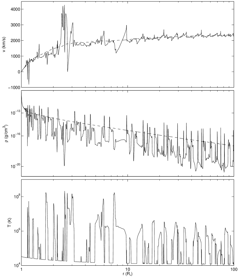
Figure 1: Velocity, density and temperature for a radiatively driven model. The dashed lines in the two upper panels represent the time-averaged variable.

In summary, we can say that the amount of clumping in our simulations is largely determined by the grid spacing, the floor temperature and $\kappa_{\rm max}$. On the other hand, we find that the clumping does not depend on the radiative force beyond $\sim 30\;R_{\ast}$ (Paper I). This reduces the outer evolution of structure to a pure gasdynamical model. As the evaluation of the radiative force dominates the computation time, this allows us to construct vastly more economical models, which we present in the following section.

3 A pseudo-planar moving periodic box formalism

3.1 Motivation and outline

Even without the evaluation of the radiative force, the modelling of structure out to very large distances ($\sim\leavevmode\nobreak\ 1000\;R_{\ast}$) is still expensive and the fine grid spacing needed to resolve the shells results in impractically large files. While such models are marginally feasible in 1D, generalizing them to higher dimensions would be computationally prohibitive. In this section, we present a technique that does not suffer from this disadvantage, and has considerable conceptual benefits.

First, let it be noted that the structure generated by the instability, apart from being stochastic, is also quasi-regular in the sense that similar features are repeated over time. Therefore it is not necessary to keep track of the whole stellar wind during the duration of the simulation. It is enough to select a limited but representative portion of the structure, and follow this as it moves out with the flow. Following a portion of the wind entails transforming the conservation equations to a moving reference frame. This is not possible directly, as the spherical equations of hydrodynamics are not invariant under a Galilean transformation. This problem can be circumvented by rewriting the equations in a pseudo-planar form (see below).

A fundamental point in the present analysis is that the time-dependent hydrodynamical variables can be viewed as having two distinct components, varying on different scales. The first is a rapidly oscillating variable, varying on short spatial and temporal scales. The second is a slowly varying function of radius, corresponding to the secular evolution of the time-averaged variable. As an example, consider the density in Fig. 1. The gas in this simulation is highly clumped, with density variations of several orders of magnitude over less than a stellar radius. The time-averaged density however, is a much more well-behaved function, decreasing steadily outward. Indeed, one of the more reassuring properties of the models including the deshadowing instability is that the mean variables closely resemble the results from CAK theory. In our pseudo-planar reformulation of the hydrodynamical equations we try to absorb, as much as possible, the secular evolution in the scaling of the variables.

3.2 Pseudo-planar scaling

For the sake of clarity, let us recapitulate the spherical equations of hydrodynamics. In Eulerian form, the one-dimensional (1D) time-dependent equations for conservation of mass, momentum, and energy are:

$$\frac{\partial\rho}{\partial t}+\frac{1}{r^{2}}\frac{\partial(r^{2}\rho v)}{\partial r} = 0$$ (2)

$$\frac{\partial(\rho v)}{\partial t}+\frac{1}{r^{2}}\frac{\partial(r^{2}\rho v^{2})}{\partial r} = -\frac{\partial p}{\partial r}+f$$ (3)

$$\frac{\partial e}{\partial t}+\frac{1}{r^{2}}\frac{\partial(r^{2}ev)}{\partial r} = -\frac{p}{r^{2}}\frac{\partial(r^{2}v)}{\partial r}-Q.$$ (4)

Here $f$ is the sum of the external forces (gravity and radiative driving) acting on the gas and $Q$ the power emitted by radiation per unit volume. The internal energy density $e$ (in erg/cm³) is related to the pressure by the perfect gas law $p=(\gamma-1)e=\rho kT/(\mu m_{\rm H})$, which supplements the set of equations. The other symbols have their usual meaning. In this paper, we assume a perfect monatomic gas and use $\gamma=5/3$ , unless otherwise specified.

The first step in our reformulation of the equations of hydrodynamics is to scale out, as much as possible, the secular components of the density, velocity and pressure. From the continuity equation it can be seen that the secular expansion of the gas at large distances from the star (where we have reached the terminal velocity) causes the density to fall of as $1/r^{2}$. This suggests the following definition of the scaled density $\tilde{\rho}$:

$$r_{0}^{2}\tilde{\rho}=r^{2}\rho,$$ (5)

where $r_{0}$ is a fiducial radius. As the mean temperature in the present models is almost constant, it is logical to scale the pressure in the same manner as the density. The scaled internal energy then follows from the perfect gas law $\tilde{p}=(\gamma-1)\tilde{e}$. The mean velocity in the outer wind is roughly constant and need not be scaled.

Rewriting Eqs. (2)-(4) in terms of the scaled variables, we obtain the following conservation equations:

$$\frac{\partial\tilde{\rho}}{\partial t}+\frac{\partial\left(\tilde{\rho}v\right)}{\partial r} = 0$$ (6)

$$\frac{\partial\tilde{\rho}v}{\partial t}+\frac{\partial\left(\tilde{\rho}v^{2}\right)}{\partial r} = -\frac{\partial\tilde{p}}{\partial r}+\tilde{f}+\frac{2\tilde{p}}{r}$$ (7)

$$\frac{\partial\tilde{e}}{\partial t}+\frac{\partial\left(\tilde{e}v\right)}{\partial r} = -\tilde{p}\frac{\partial v}{\partial r}+\tilde{Q}-\frac{2\tilde{p}v}{r},$$ (8)

where the external force and the heating rate have been scaled in the same way as the density and the pressure. These equations are pseudo-planar in the sense that they describe the spherical problem but formally resemble the planar equations of hydrodynamics. The only formal difference with the planar equations are the geometric source terms appearing in the momentum and energy equations. These express the secular evolution of momentum and energy in spherical geometry. The outer wind is essentially expanding at a constant velocity while the temperature is kept constant by the balance between heating and cooling. The geometric source term $2\tilde{p}/r$ in the momentum equation represents the pressure gradient associated with this secular expansion. The geometric source term $2\tilde{p}v/r$ in the energy equation expresses the secular adiabatic cooling of the gas.

3.3 Transformation to moving box

Let us now transform the pseudo-planar equations from the stellar rest frame to a frame that is moving at a constant velocity $v_{0}$. We refer to this moving frame as the box. We define the position coordinate $x$ within the box by the Galilean transformation

$$r=R_{0}+v_{0}t+x,$$ (9)

where $R_{0}$ is the initial inner radius of the box. For any variable $\alpha$ depending on position and time we can then convert from $\alpha(r,t)$ to $\alpha(x,t)$. We denote the time-derivative at constant $x$ by ${\rm d/d}t$. We then have

$$\frac{\rm d\alpha}{{\rm d}t}\equiv\left.\frac{\partial\alpha}{\partial t}\right|_{x}=\left.\frac{\partial\alpha}{\partial t}\right|_{r}+\left(\@vec{v_{0}}\cdot\@vec{\nabla}\right)\alpha$$ (10)

If we further introduce the velocity $w$ with respect to the box velocity, i.e. $v=v_{0}+w$, then we can rewrite the equations of hydrodynamics as

$$\frac{\rm d\tilde{\rho}}{{\rm d}t}+\frac{\partial\left(\tilde{\rho}w\right)}{\partial x} = 0$$ (11)

$$\frac{\rm d\left(\tilde{\rho}w\right)}{{\rm d}t}+\frac{\partial\left(\tilde{\rho}w^{2}\right)}{\partial x} = -\frac{\partial\tilde{p}}{\partial x}+\tilde{f}+\frac{2\tilde{p}}{R_{0}+v_{0}t+x}$$ (12)

$$\frac{{\rm d}\tilde{e}}{{\rm d}t}+\frac{\partial\left(\tilde{e}w\right)}{\partial x} = -\tilde{p}\frac{\partial w}{\partial x}+\tilde{Q}-\frac{2\tilde{p}(v_{0}+w)}{R_{0}+v_{0}t+x}$$ (13)

Finally, we impose periodic boundary conditions on the box. The box method has a number of advantages that should be clear already. Not only is the number of grid points reduced with respect to a traditional calculation where the whole wind is evolved, it is also not necessary to increase the number of depth points if the structure needs to be followed further. The computing time is less, due to the smaller number of grid points. Furthermore, any explicit time-stepping method is subject to a stability condition on the Courant number $C=c\Delta t/\Delta x$, where $c$ is the maximum propagation speed of information, $\Delta t$ the time step and $\Delta x$ the grid spacing. In order to be stable, $C$ must be smaller than one (this is the Courant-Friedrichs-Lewy condition), and preferably a lot smaller. Due to the slower speed at which features are advected over the numerical grid, the condition on the Courant number is less restrictive for the box model. The gain is substantial: permitted time steps increase from $\sim\Delta x/v_{\infty}$ to a few times $\Delta x/a$, where $a$ is the sound speed. In the simulations presented here, $v_{\infty}/a\approx 150$.

3.4 Effect of periodic boundary conditions

General principles

As a consequence of the periodic boundary conditions, structure is always dragged along with the box. To ensure that the time scale over which the structure evolves is comparable to the time-scale associated with its outward movement, the speed of the box must be roughly the same as the terminal velocity. This is clear from the fact that it is obviously not possible to evolve structure cheaply by taking a very large box speed. Furthermore, as shell collisions are very important for the evolution of structure (Paper I), the box should be big enough to contain more than one shell, even at late times. Finally, the periodic boundary conditions move features such as dense shells from one side of the box to the other. The box method is inherently incapable of describing variations on scales beyond a box length. This means that the length of the box should be small compared to the distance covered by the box.

Restriction of box size from energy equation

A quantitative restriction on the box size can be derived from the secular change of the energy density over the length of the box. Using the energy equation (13) we can write the relative change in the secular component of the energy density over a box length $L$ as

$$\epsilon_{\rm e}\equiv\frac{1}{\tilde{e}}\int_{0}^{\tau}\frac{2\tilde{p}(v_{0}+w)}{R_{0}+v_{0}t+x}dt,$$ (14)

where $\tau=L/v_{0}$. If we assume that the change in $\tilde{p}$ is slow compared to $1/t$ this gives

$$\epsilon_{\rm e}=2(\gamma-1)\ln\left(1+\frac{L}{R_{0}+x}\right).$$ (15)

Using $x=L/2$ and $R_{0}=50R_{*}$ the requirement $\epsilon_{\rm e}<0.25$ gives $L<11.5R_{*}$.

Restriction from clumping factor

A different measure of the effect of periodic boundary conditions is given by their influence on the clumping factor. When a shell crosses the boundary of the box, it effectively jumps a distance $L$ in the stellar rest frame. If the clumping factor changes over length scales $\sim L$, this introduces an error, which we can estimate in the following simplified model. Let us assume a single shell in the box, with an expansion speed $a_{\rm e}$. If the shell has a width $l_{\rm L}$ at the left side of the box then it has a width $l_{\rm L}+\Delta l$ at the right side of the box, where $\Delta l=a_{\rm e}L/v_{\infty}$. Note that the relevant time-scale for the expansion is not the time needed for the shell to cross the box, but the much shorter time $L/v_{0}$ needed for the shell to move a distance $L$ in the stellar rest frame. We can then write the relative change in the clumping factor caused by applying the periodic boundary conditions as

$$\epsilon_{\rm cl}\equiv\frac{f_{\rm cl,L}-f_{\rm cl,R}}{f_{\rm cl,R}}=\frac{a_{\rm e}}{v_{\infty}}\frac{L}{l_{\rm L}},$$ (16)

where we have used the fact that the clumping factor can be approximated by the inverse of the volume filling factor, which in turn is the fractional width occupied by the shell (see e.g. Paper I). This equation shows that the error caused by applying periodic boundary conditions is large if the shells expand fast, the outflow velocity is small, the box is big or the shells are narrow. This last possibility is explained by the fact that for a given $L,a_{\rm e}$ and $v_{\infty}$, the expansion $\Delta l$ is constant and therefore relatively more important for narrow shells. From the models presented later in this paper (Sect. 6), we can derive typical values to use in Eq. (16). At $\approx 170R_{*}$, where the first shell crosses the box (Fig. 11), the clumping factor is less than 10. For an expansion speed of 50 km/s and a terminal speed of 2300 km/s we have $\epsilon_{\rm cl}\approx 20\%$, i.e. for the model parameters used in this paper, the error on the clumping factor caused by applying the periodic boundary condition is less than $20\%$. The assumption of a single shell is not a limitation, because the above analysis can be repeated for any number of shells to obtain the same result.

3.5 Implementation

We have implemented the pseudo-planar periodic box technique in VH-1, a hydrodynamics programme (or hydrocode) developed at the University of Virginia (Blondin, personal communication). This code solves the Eulerian equations of hydrodynamics by a Lagrangian remap (LR) method, which first solves the Lagrangian equations of hydrodynamics and then maps the updated quantities back onto the Eulerian grid. A major challenge in Eulerian hydrodynamics, even in their LR incarnation, is to obtain reliable estimates of time-averaged quantities such as pressure and density at zone interfaces. All quantities in VH-1 are zone-centred, i.e. VH-1 does not use a staggered mesh. To determine the time averages, a Riemann problem (Zel’dovich & Raizer Zeldovich&Raizer (1966)) is set up, and solved, at each zone interface. A parabolic interpolation is used to provide an accurate guess to the values on either side of the interface. This combination of the parabolic interpolation and the Riemann solver is referred to as the piecewise parabolic method (PPM; Colella & Woodward CW84 (1984)) and is the heart of VH-1. The details of the implementation are described in Paper I, the obvious exception being that the radiative force need not be evaluated in the present work.

4 Test problems

4.1 Uniformly expanding sphere

A straightforward problem to test the pseudo-planar approach is that of an expanding sphere with spatially constant density and pressure, and a radially increasing velocity (see e.g. Blondin & Lufkin BL93 (1993)). For an initial condition with density $\rho_{0}$, pressure $p_{0}$ and velocity $v=r/t_{0}$ this problem has the analytic solution

$$\rho=\rho_{0}\left(\frac{t_{0}}{t}\right)^{3},\qquad v=\frac{r}{t},\qquad p=p_{0}\left(\frac{t_{0}}{t}\right)^{3\gamma}.$$ (17)

This test problem was used by Blondin & Lufkin to illustrate the use of geometry corrections to minimise advection errors near the origin of a curvilinear coordinate system. For the present simulation, we have used the version of VH-1 available from the North Carolina State University website. This version does not include the geometry corrections. To avoid problems with the derivation of the internal energy from remapped quantities, Blondin & Lufkin removed the pressure gradient from the momentum equation. For the pseudo-planar method, this would also remove the geometrical source term from Eq. (7), thus greatly reducing the stringency of our test. We therefore include the pressure gradient in our calculations.

As a point of reference, we choose an initial condition that produces physical parameters typical for the outer wind of a hot star:

$$t_{0}=10^{5}\mathrm{s},\quad\rho_{0}=10^{-16}\mathrm{g/cm^{3}},\quad p_{0}=5\times 10^{-4}\mathrm{dyn/cm^{2}}.$$ (18)

The spatial grid has 96 points and extends from 0.1 to 3.1 $R_{\ast}$, where $R_{\ast}=19\;R_{\sun}$. We compare both a spherical model, calculated by solving Eqs. (2)-(4), and a pseudo-planar model in a stationary box, calculated by solving Eqs. (6)-(8), with the exact analytical solution. The Courant number is 0.25. The boundary conditions were chosen so as to impose a zero gradient on density and pressure, and a constant gradient on the velocity. In the case of the pseudo-planar method, the scaled variables (e.g. $\tilde{\rho}$) are implicitly scaled back to their physical counterpart ($\rho$) before imposing the boundary condition. This is important when comparing the two methods, as a difference in the quality of the boundary conditions would swamp the relatively small errors intrinsic to the method. Figure 2 shows that the pseudo-planar model performs marginally better than the spherical model. This is gratifying, as the test is unfavourable to the pseudo-planar method, which has to produce a flat physical density and pressure by evolving a curved rescaled density and pressure.

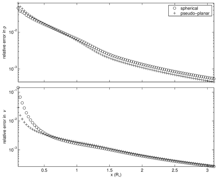
Figure 2: Relative difference between the analytic solution and the computer simulation for the uniformly expanding sphere test problem. Upper panel: density. Lower panel: velocity.

4.2 A moving shock tube in planar geometry

The Sod shock tube (Sod Sod (1978)) has become a standard test for all hydrodynamics codes. It is a special case of the Riemann problem, describing the evolution of an arbitrary discontinuity (Zel’dovich & Raizer Zeldovich&Raizer (1966)). A hypothetical membrane separates two regions of uniform density, pressure and velocity, where at least one of these quantities is different on either side of the membrane. At $t=0$, the membrane is removed and the jump discontinuity breaks up into a shock wave, a contact discontinuity and a rarefaction wave. In planar geometry, this problem has a semi-analytical solution (Sod Sod (1978), Laney Laney (1998)). The standard problem presented by Sod, with the gas at rest at both sides of the membrane, a density ratio of 8 and a pressure ratio of 10, is quite unchallenging for any modern hydrocode. The physical problems to which these codes are applied generally present more extreme conditions.

In radiatively driven stellar winds, density contrasts are often orders of magnitude larger than in the standard Sod problem, while the gas moves over the grid at supersonic speeds. We therefore propose a shock tube with a density ratio of 800 and a pressure ratio of 1000, with all of the gas initially moving at the same supersonic speed. By Galilean invariance, the solution should not depend on this initial speed (except for an obvious displacement). On one side of the membrane, we have $\rho_{l}=100$, $p_{l}=100$, $u_{l}=60$, on the other $\rho_{r}=0.125$, $p_{r}=0.1$, $u_{r}=60$. Furthermore, to highlight possible differences between forward and reverse waves, we set two such shock tubes back to back, so that we have shocks, contact discontinuities and rarefaction waves running in both directions. The initial situation is a layer of dense, high-pressure gas separated by two membranes from the surrounding sparse, low-pressure gas, with everything moving at the same speed. The original thickness of the dense layer is 0.2.

The initial speed is more than fifty times the adiabatic sound speed (the value of the adiabatic constant in this problem is 1.4). This is a more challenging test than the standard Sod problem, but by no means more extreme than the conditions in a stellar wind. In Fig. 3 we compare the

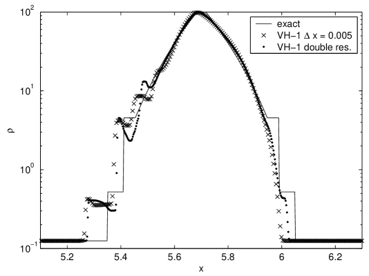
Figure 3: A VH-1 solution of the density for the moving shock tube problem. The exact solution (solid line) is compared to a VH-1 simulation with resolution $\Delta x=0.005$ (crosses) and $\Delta x=0.0025$ (dots).

analytical solution (solid line) with the numerical solution using VH-1 in planar geometry, with a step size of 0.005 (crosses) and a Courant number of 0.25. The results are quite dismal, particularly for the inward rarefaction, which shows a lot of unphysical substructure. Note also that the inward running shock is not at the correct position.

This substructure is present for a wide range of code parameters. Increasing the resolution by a factor of two (dots) gives an unsubstantial improvement, as do variations in the restriction on the Courant number (we repeated the calculation with Courant numbers between 0.1 and 0.6 and found similar results). The artefacts occur regardless of whether the internal energy is remapped separately or derived from the remapped total energy (see below). They also occur for a wide range of shock flattening parameters (see below)

In hot-star wind simulations, the internal energy is an ill-conditioned part of the total energy (Feldmeier Feldmeier95 (1995)). We found that deriving the internal energy from the remapped total energy can result in artificial spikes of low temperature. To alleviate this problem one can remap both the internal and total energy, and derive the internal energy from the total energy only when the Mach number of the flow is sufficiently low (Blondin, personal communication). We found that, though this fix is important in our radiatively driven calculations, it does not help with the artefacts shown in Fig. 3 . Indeed, the models shown includes this fix, which at $M=60$ means that the internal energy is never determined using the total energy. When the total energy is used, the results are worse.

We find that shock flattening (Colella & Woodward CW84 (1984)) does little to improve the results. This technique flattens the interpolating parabola in the vicinity of a shock. In the calculations presented here we have used the flattening parameters $\omega^{(1)}=0.75$, $\omega^{(2)}=5.0$ and $\epsilon=0.33$. Even with extreme shock flattening ($\omega^{(1)}=0$, $\omega^{(2)}=10.0$ and $\epsilon=0$) the artefacts do not disappear, and the amount of smearing at the shocks is unacceptable. Flattening is usually only applied in the Lagrangian hydro step. Extending flattening to the remap step doesn’t improve the results substantially. If the interpolating function is totally flattened in very grid point (i.e. by setting the flattening coefficient $f_{i}=1$ for all $i$), VH-1 reproduces the Godunov scheme. In this case, all features in the test problem are completely wiped out, because the scheme is too dissipative. By trial and error we find that setting the flattening coefficient $f_{i}=0.025$ for all $i$ gives acceptable results.

As a comparison, we ran the same simulation using ZEUS, a widely used MHD code developed by Stone & Norman (SN92 (1992)). The numerical algorithms used to solve the Eulerian equations in ZEUS are quite different from those adopted in VH-1. It does not use a Lagrangian remap, but directly solves the Eulerian equations. The solution is split into two parts: a source step and an advection step. Although a staggered mesh is used, interpolations are still needed to determine the time-averaged values of variables at zone interfaces. ZEUS provides a second-order method (Van Leer) and a third-order method (PPA, for piecewise parabolic advection). Note that PPA is only half of PPM, as it incorporates the parabolic interpolation, but not the Riemann solver. We have applied both the Van Leer scheme and PPA to the moving shock tube problem. Figure 4 shows that the Van Leer scheme (crosses) does much

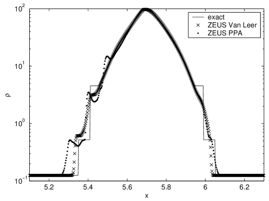
Figure 4: Two ZEUS solutions of the moving shock tube problem. The exact solution (solid line) is compared to a ZEUS calculation using the Van Leer scheme (crosses) and a calculation using PPA (dots).

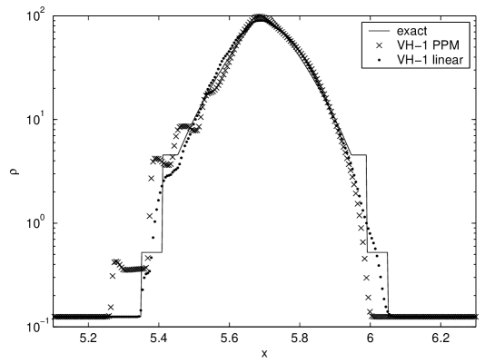
Figure 5: Two VH-1 solutions of the moving shock tube problem. The exact solution (solid line) is compared to a a standard VH-1 calculation using PPM (crosses) and a calculation using linear interpolation (dots).

better on this problem than VH-1, while PPA (dots) produces the same kind of unphysical substructure. The resolution used in this calculation is $\Delta x=0.0025$. At a resolution of 0.005 (not shown on figure), the Van Leer scheme doesn’t manage to capture the shock and the contact discontinuity, but doesn’t produce any spurious features either. Given the differences between the two codes, it is quite surprising that the artefacts in VH-1 and ZEUS PPA are so similar. It strongly suggests that they are the result of the parabolic interpolation scheme used in both codes. To confirm this, we artificially lowered the order of VH-1 by setting the quadratic term in the interpolating function to zero. The results for the linear interpolation scheme are much better than for the higher order PPM (Fig. 5). The difference is due to errors in the remap step. This can be seen from the fact that using linear interpolation in the remap step only gives essentially the same results.

The artificial substructure in this test problem is similar to the rarefaction shocks found by Falle (Falle (2002)) in a ZEUS test calculation of a different Riemann problem, using the Van Leer scheme. We have found, as expected, that VH-1 performs very well on Falle’s test problem and that using PPA in ZEUS also produces artefacts.

Figure 6 shows the density and the isothermal sound speed for a VH-1 simulation using the pseudo-planar method. The pseudo-planar method, by its very nature, can only solve problems in a spherical geometry. Planar geometry was mimicked by taking a very large initial position of the box. The box velocity was taken equal to the initial speed of the gas. The pseudo-planar method (crosses) is compared to the exact solution and to the ZEUS Van Leer simulation described above. It is clear that the pseudo-planar method performs very well on this test problem. This shows that the main stumbling block for VH-1 and ZEUS PPA is the supersonic velocity with which the features move over the grid. Indeed, any box velocity reducing this velocity to less extremely supersonic values gives adequate results.

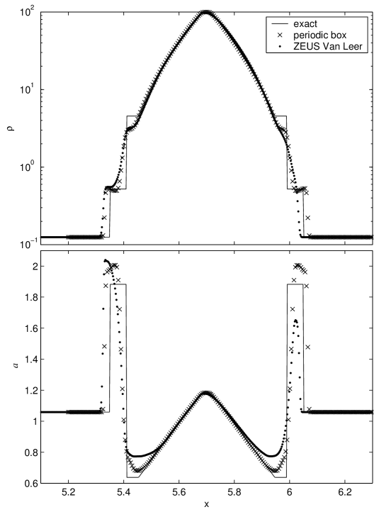
Figure 6: Density and sound speed for a periodic box solution of the moving shock tube problem. The periodic box method (crosses) is compared to the exact solution (solid line) and the ZEUS Van Leer method (dots).

With minor modifications, VH-1 can also be used as a pure Lagrangian code. In this mode, the results are of the same quality as those of the periodic box technique, which corroborates the above conclusion.

In summary, we can say that the combination of parabolic interpolation and highly supersonic advection leads to unphysical substructure and incorrect shock speeds. The results can be improved by removing the advection from the scheme (e.g. by using the periodic box technique) or by avoiding parabolic interpolation. The lesson to be drawn from these experiments is that for problems that are rapidly advected over the computational grid, higher order schemes such as PPM do not necessarily give more accurate results than lower-order schemes.

5 Application to stellar winds

5.1 Initial condition

To apply the moving periodic box simulation we select as an initial condition a region from the snapshot shown in Fig. 1. The region is chosen so that it contains a sufficiently large number of shells. This is necessary to be able to evolve a model over a long period of time, as the evolution of the structure is largely determined by the fact that shells in the box collide and form denser shells as the box moves outward, counteracting their pressure-expansion. If only a single shell remains, the calculation becomes meaningless as there is obviously no opportunity for further collisions. The boundaries of the box were set to generate a periodic velocity. The density and pressure were then slightly modified near the inner boundary of the box, to ensure periodicity in the corresponding scaled variables and thereby avoid introducing any additional discontinuities. In practice, the initial condition is the region $r=46.1\leavevmode\nobreak\ -\leavevmode\nobreak\ 94\;R_{\ast}$ on the snapshot. The scaled density is made periodic by introducing a linear “correction” between the inner boundary and some $r_{1}$, so that the modified scaled density is the same at the left and right boundaries and the correction vanishes at $r_{1}$. The pressure is made periodic in the same manner. Points beyond $r_{1}$ are not modified. In the simulations shown $r_{1}=49.2\;R_{\ast}$.

5.2 Comparison with radiatively driven model

5.2.1 Stationary periodic box

To better evaluate possible differences between a moving periodic box model and the standard radiatively driven model, we first apply the pseudo-planar equations in a stationary periodic box. We can compare the stationary periodic box model with the driven model only in a limited region of the $r,t$ plane. This is illustrated in Fig. 7. The wide box represents the domain in space and time covered by a radiatively driven model. The tall box represents the domain covered by a stationary box model. In principle, the two models can be compared in the square region where they overlap. However, the two models use different boundary conditions, so the comparison is only meaningful in the region that depends exclusively on the initial condition and not on the boundary conditions. This region is the filled triangle in Fig. 7. The upper edge of this triangle is in fact a $C_{+}$ characteristic (see e.g. Zel’dovich & Raizer Zeldovich&Raizer (1966)), along which a signal from the inner boundary condition is carried outward. It need not be a straight line. In the context of the present paper it can be viewed as the outer edge of an expanding shell and the upshot of the above is that we can only compare the box model with the driven model for shells that have not crossed the boundary of the box.

Figure 8 shows a snapshot at 100 ksec, for a stationary periodic box model (solid line) and a radiatively driven model (dashed line). We show only the region in $r$ where the comparison is meaningful. It is clear that the two models agree very closely. The small differences are most obvious in the velocity plot (upper panel) and appear to be due to the residual level of radiative driving beyond $45\;R_{\ast}$.

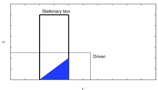
Figure 7: Regions in the space-time plane covered by a full radiatively driven model and a stationary periodic box model. The dark triangle indicates the area in space-time covered by both models, i.e. the area where results of the models can be compared

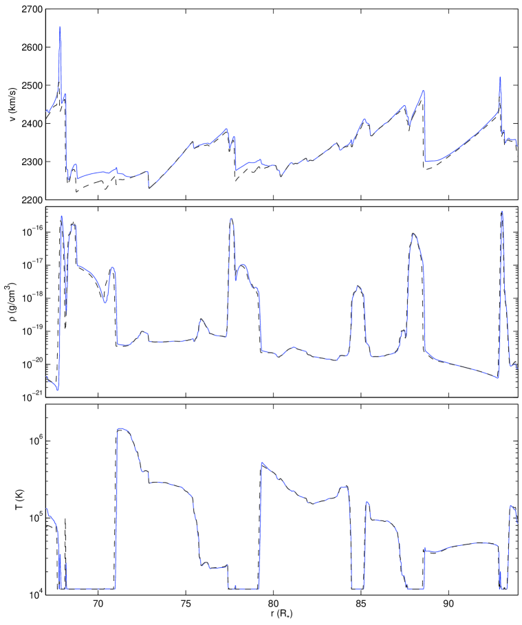
Figure 8: Snapshot of velocity, density and temperature at 100 ksec for a radiatively driven model (solid line) and a stationary periodic box model (dashed line)

5.2.2 Moving periodic box

Let us now compare the results for a moving periodic box model with a radiatively driven model. Figure 9 shows the domains in the r,t plane covered by the moving box model and the radiatively driven model. The region (filled) where the two can be meaningfully compared is somewhat larger than for the stationary box, but still limited, this time by both $C_{+}$ and $C_{-}$ characteristics. Again, the meaningful region can be viewed as those shells that have not crossed the boundary of the box.

Figure 10 shows a snapshot at 100 ksec, for a moving periodic box model (solid line) and a radiatively driven model (dashed line). It is clear that the agreement is less than perfect. In particular, the temperature of the moving box model shows features that are not present in the driven calculation. Both models have broad regions of rarefied hot gas (such as the one extending from 79 to 84.5 $R_{\ast}$). This is gas that has been previously heated and has remained hot due to the inefficiency of radiative cooling at low densities. (We recall that we solve the energy equation including radiative cooling, using the Raymond et al. [RCS (1976)] cooling curve). In addition to these broad warm regions, the periodic box model has narrow regions of gas heated by nearby shocks. The most conspicuous pair of such narrow, hot regions is centred around 90 $R_{\ast}$. These narrow regions are not present in the case of a stationary periodic box. They appear due to the Galilean transformation which is the only difference between the moving and stationary periodic box calculations. These narrow regions are perfectly physical: the left region is heated by the forward shock at $\approx 89\;R_{\ast}$, the right region by the reverse shock at $90.5\;R_{\ast}$. Their narrowness is explained by the fact that the shocks have only been able to heat the gas during a 100 ksec time interval, and is consistent with the velocity at which the gas flows out of the shock. It is in fact their absence in the radiatively driven calculation that is disturbing. As gas passes through a shock, part of its kinetic energy is converted into internal energy. As it moves away from the shock, the shock-heated gas cools by emitting radiation. A useful expression for the length of the cooling zone was given by Feldmeier (Feldmeier95 (1995)). Using his Eq. (A9) we find that the cooling length for even the weakest outer-wind shocks is well-resolved by the numerical grid. The cooling length for the relatively strong ($\chi=3.7$) reverse shock at $90.5\;R_{\ast}$ in Fig. 10 is a huge $400\;R_{\ast}$!

The absence of hot gas behind the shocks of the radiatively driven and stationary periodic box model is a manifestation of the “collapse” of cooling zones. This is a problem that has plagued all hydrodynamical simulations of hot-star winds that include energy balance. It has been attributed to a global thermal instability leading to an oscillation of the width of the cooling zone (Feldmeier Feldmeier95 (1995)) and to advective diffusion (Cooper CooperPhD (1994)). Advective diffusion is caused by the combination of advection with the typical shape of the cooling curve. Between $10^{5}$ and $10^{7}$ K, this curve falls off as $T^{-1/2}$. When a steep temperature feature is advected over the grid, it is inevitably smeared by numerical diffusion. Due to the $T^{-1/2}$-dependence of the cooling, the cold side of the smeared-out feature cools more rapidly than the warm side. This effectively steepens the feature again, but also makes it narrower. In this way, the numerical scheme takes a bite out of the cooling zone at every time-step, until it is eaten away completely. Our results suggest that, at least in the outer wind, advective diffusion is the cause of the collapse of the cooling zones.

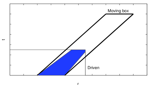
Figure 9: Regions in the space-time plane covered by a full radiatively driven model and a moving periodic box model. The dark trapezium indicates the area in space-time covered by both models, i.e. the area where results of the models can be compared

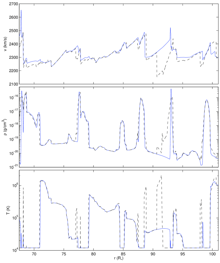
Figure 10: Snapshot of velocity, density and temperature at 100 ksec for a radiatively driven model (solid line) and a moving periodic box model (dashed line)

6 Results for an example application

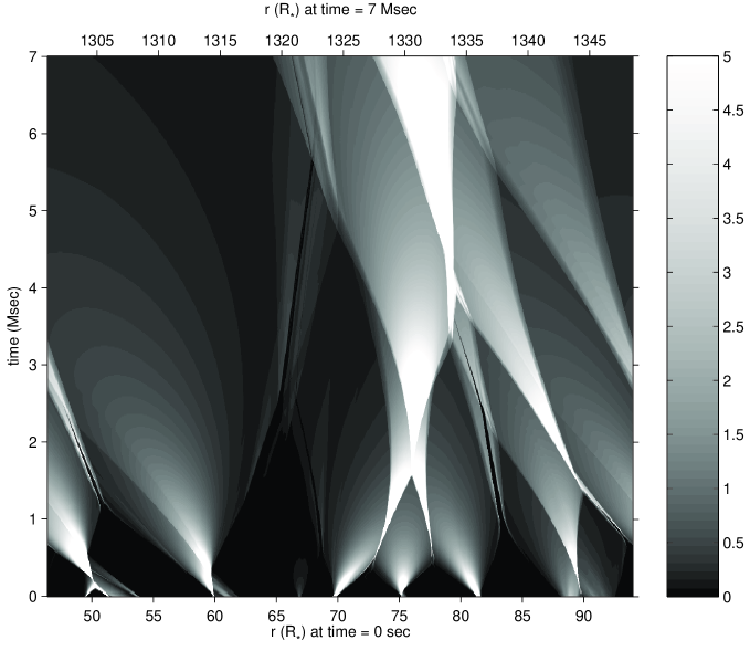
Figure 11: Greyscale image of the density contrast (density divided by mean density) as a function of space and time. The intensity scale has been truncated to highlight the kinematics of the shells.

Let us now apply the periodic box technique to the problem it was designed for: the evolution of stellar wind structure out to very large distances. In Fig. 11 we show the evolution of the density contrast (density divided by mean density) as a greyscale image. During the 7 Msec interval shown, the box moves from 50 to 1300 $R_{\ast}$. This figure shows the considerable conceptual advantage of the periodic box method. By following a fraction of the wind as it moves away from the star, the relevant physical mechanisms (pressure expansion and shell collisions) are immediately apparent. Similar greyscale images can be made for the other variables.

The evolution of structure can be usefully described by a number of statistical quantities, such as the clumping factor and the velocity dispersion. These descriptors have been defined in Paper I, and involve the temporal average of variables such as the density at a given position in the wind. This is somewhat cumbersome in a moving box model, because a given position in the wind does not correspond to a unique position within the moving box, and calculating a time average requires some awkward bookkeeping. It is more convenient to replace the temporal averages by spatial averages using the following ergodic approximation

$$v_{0}\int_{t-T}^{t}\rho(x,t^{\prime}){\rm d}t^{\prime}\approx\int_{x}^{x+X}\rho(x^{\prime},t){\rm d}x^{\prime},$$ (19)

which holds if the statistical properties remain stationary over a time $\Delta t=L/v_{\rm b}$. We can then calculate the clumping factor and the velocity dispersion, which are shown in Fig. 12.

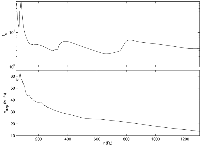
Figure 12: Clumping factor and velocity dispersion as a function of radius for the box model.

The velocity dispersion declines gradually to reach values barely above the sound speed ($\approx 13$ km/s), although the strongest shock in the final state still has a jump velocity of 25 km/s (Fig. 13). The clumping factor has the oscillating behaviour typical of the competition between pressure expansion and shell collisions. Between 200 and 1300 $R_{\ast}$, the clumping factor ranges from 2.5 to 6.

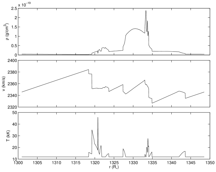
Figure 13: Snapshot of density, velocity and temperature at the end of the box simulation (7 Msec).

These simulations show that, within the 1D assumption, the wind remains structured over huge distances. Observational diagnostics such as radio emission (both thermal and non-thermal) are inevitably influenced. Inferred mass-loss rates, that scale as $\sqrt{f_{\rm cl}}$ would be overestimated by a factor of around two. It appears plausible, again within the approximations, that shocks survive out to the large distances needed to explain the non-thermal radio emission.

7 Summary

We have presented an efficient technique to study the evolution of instability-generated structure far away from the star. Because it follows a small part of the structure, high spatial resolution can be maintained with a relatively small number of points. Furthermore, the number of depth points required does not depend on the time-span of the simulation. The small number of points makes for smaller files and facilitates the analysis of the results. As the box follows the flow, the gas is advected over the grid at much lower speeds than in a traditional model. This makes the condition on the Courant number much less restrictive, resulting in a substantial reduction in computation time. The moving box also has a conceptual advantage, in that it makes it easier to visualise the physical processes that are happening in the simulation.

We have shown that the high Mach numbers with which the gas moves over the grid in traditional models are a cause for concern, as it can cause unphysical structure to appear, and physical structure to disappear. In this sense, the box model is not only faster, but also more accurate. It is therefore a useful tool to check whether a solution depends on the Galilean frame in which it is obtained. Using the box model, we have shown that the wind remains clumped out to $1300\;R_{\ast}$ and that weak shocks remain present.

A key limitation of the present method is its restriction to just one-dimension (1D), with focus on the extensive structure in radius, but not accounting at all for likelihood that in 2D or 3D models, Rayleigh-Taylor or thin-shell instabilities would break up the assumed azimuthal coherence (Vishniac Vishniac (1994)). Future work should thus focus on extending these period box techniques to 2D or 3D, in conjunction with recent efforts to develop multi-dimensional radiation-hydrodynamics simulations of the initial formation of structure arising from the line-deshadowing instability (Dessart & Owocki Dessart+ (2003); Gomez & Williams Gomez+ (2003)).

- (1) Blondin, J. M. & Lufkin, E. A. 1993, ApJS, 88, 589
- (2) Bunn, J. C. & Drew, J. E. 1992, MNRAS, 255, 449
- (3) Colella, P., Woodward, P. 1984, J. Comput. Phys., 54, 174
- (4) Cooper, R. G. 1994, Ph.D. Thesis, Univ. of Delaware
- (5) Dessart, L. & Owocki, S. P. 2003, A&A, 406, L1
- (6) Drew, J. E. 1989, ApJS, 71, 267
- (7) Falle, S. A. E. G. 2002, ApJ, 577, L123
- (8) Feldmeier, A. 1995, A&A, 299, 523
- (9) Feldmeier, A. 2001, Habilitation Thesis, University of Potsdam
- (10) Feldmeier, A., Puls, J., Pauldrach, A.W.A. 1997, A&A, 322, 878
- (11) Gomez, E. L. & Williams, R. J. R. 2003, MNRAS, 344, 725
- (12) Grosdidier, Y., Moffat, A. F. J., Joncas, G., & Acker, A. 1998, ApJ, 506, L127
- (13) Hillier, D. J., Kudritzki, R. P., Pauldrach, A. W., Baade, D., Cassinelli, J. P., Puls, J., & Schmitt, J. H. M. M. 1993, A&A, 276, 117
- (14) Kramer, R. H., Cohen, D. H., & Owocki, S. P. 2003, ApJ, 592, 532
- (15) Laney, C.B. 1998, Computational Gasdynamics, Cambridge University Press
- (16) Owocki, S. P. & Rybicki, G. B. 1984, ApJ, 284, 337
- (17) Owocki, S. P., Castor, J. I., & Rybicki, G. B. 1988, ApJ, 335, 914
- (18) Runacres, M. C, & Owocki, S. P. 2002, A&A, 381, 1015 (Paper I)
- (19) Raymond, J. C., Cox, D. P., & Smith, B. W. 1976, ApJ, 204, 290
- (20) Sod, G. A 1978, J. Comp. Phys. 27, 1
- (21) Stone, J. M. & Norman, M. L. 1992, ApJS, 80, 753
- (22) Van Loo, S., Runacres, M. C., & Blomme, R. 2004, A&A, submitted
- (23) Vishniac, E. T. 1994, ApJ, 428, 186
- (24) Zel’dovich, Y. B., Raizer, Y. P. 1967, Physics of Shock Waves and High-Temperature Hydrodynamic Phenomena, Vol. I, Academic Press, New York