The abundance of Lyman-$\alpha$ emitters in hierarchical models

Abstract

We present predictions for the abundance of Ly-$\alpha$ emitters in hierarchical structure formation models. We use the GALFORM semi-analytical model of galaxy formation to explore the impact on the predicted counts of varying assumptions about the escape fraction of Ly-$\alpha$ photons, the redshift at which the universe reionized and the cosmological density parameter. A model with a fixed escape fraction gives a remarkably good match to the observed counts over a wide redshift interval. The counts at bright fluxes are dominated by ongoing starbursts. We present predictions for the expected counts in a typical observation with the Multi-Unit Spectroscopic Explorer (MUSE) instrument proposed for the Very Large Telescope.

1 Introduction

Dedicated narrow-band searches for Ly-$\alpha$ emitters have proven to be very efficient at detecting high-redshift galaxies (e.g. Hu & McMahon et al. 2003). Objects found by this technique have to be confirmed spectroscopically, to rule out possible low redshift interlopers that may arise due to emission lines other than Ly-$\alpha$ falling within the targetted wavelength interval. Nevertheless, a significant fraction of the detections appear to be bona-fide Ly-$\alpha$ emitters, and the number of objects accumulated to date by this technique in the redshift interval $2.4<z<6.6$ is quite impressive. The Ly-$\alpha$ emission line is also found in a significant fraction of Lyman break galaxies (e.g. which are selected on the basis of their continuum emission.

The ubiquity of the Ly-$\alpha$ line is at face value surprising, given that it is resonantly scattered by atomic hydrogen, and so is easily absorbed by even a small amount of dust in a neutral gaseous medium. It is suspected that most Ly-$\alpha$ emitters have galactic winds (as is the case with Lyman break galaxies) which allow Ly-$\alpha$ photons to escape from the galaxy after only a limited number of resonant scatterings (Kunth et al. 1998; Pettini et al. 2001). The Ly-$\alpha$ line typically shows an asymmetric profile characteristic of such a process (e.g. Ahn 2004). The physics of this phenomenon is complicated, however, and remains poorly understood.

We present here the first predictions for the abundance of Ly-$\alpha$ emitters at different redshifts made using a model which follows the formation and evolution of galaxies in a hierarchical universe. In previous work, simple, ad-hoc prescriptions have been used to assign star formation rates to dark matter haloes (Haiman & Spaans 1999; Santos et al. 2004). In this Letter, we use a semi-analytical model to make an ab initio calculation of the distribution of galaxy masses and star formation rates at different redshifts (e.g. Cole et al. 1994; Kauffman et al. 1994; Baugh et al. 1998; Somerville & Primack 1999; Hatton et al. 2003). The model we use is able to reproduce the observed properties of galaxies both locally and at high redshift [Cole et al. 2000, Baugh et al. 2004]. The abundance of Ly-$\alpha$ emitters is sensitive to the adopted cosmological model and to astrophysical phenomena, such as the fraction of Ly-$\alpha$ photons escaping from galaxies and the distribution of galactic dust. Semi-analytical models are ideally suited to the exploration of such a parameter space.

The semi-analytical model is described in Section 2. In Section 3, we first present a compilation of the available observational data on the abundance of Lyman-$\alpha$ emitters at different redshifts, and then compare these data with the predictions from our models. Finally, we present our conclusions in Section 4.

MODEL	$\Omega$	$\Lambda$	$\sigma_{8}$	$z_{\rm reion.}$	$f_{\rm esc.}$	MUSE COUNTS
A	$0.3$	$0.7$	$0.93$	$10$	$0.02$	$70$
B	$0.3$	$0.7$	$0.93$	$10$	$0.1$	$248$
C	$0.3$	$0.7$	$0.93$	$10$	dust	$366$
D	$0.3$	$0.7$	$0.93$	$6$	$0.02$	$163$
E	$0.3$	$0.7$	$0.93$	$20$	$0.02$	$77$
F	$0.2$	$0.8$	$1.15$	$10$	$0.02$	$145$
G	$1$	$0$	$0.52$	$10$	$0.02$	$59$

Table 1: The parameters of the semi-analytical models for which the abundances of Ly-$\alpha$ emitters are predicted. The first column gives the model label. The next three columns give the basic cosmological parameters: the density parameter, $\Omega$, the cosmological constant, $\Lambda$, and the amplitude of density perturbations, as specified by $\sigma_{8}$ ($\sigma_{8}$ values are taken from Eke et al. 1996). In each case the baryon density is $\Omega_{b}=0.04$ and the Hubble constant is $H_{0}=70{\rm kms}^{-1}{\rm Mpc}^{-1}$. Column five gives the redshift $z_{\rm reion}$ at which the universe is assumed to reionize. Column six gives the fraction $f_{\rm esc}$ of Lyman-$\alpha$ photons that escape from the model galaxies. In the case of model C, the escape fraction is computed from a dust extinction model, as described in the text. The final column gives the number counts of Lyman-$\alpha$ emitters for a reference MUSE observation. This is the number of emitters in 1 square arcminute in the redshift interval $2.8<z<6.7$ brighter than $3.9\times 10^{-19}{\rm ergs}^{-1}{\rm cm}^{-2}$.

2 The model

We use the semi-analytical model of galaxy formation, GALFORM, to make predictions for the abundance of Ly-$\alpha$ emitters as a function of Ly-$\alpha$ flux and redshift. The GALFORM model is described in full in Cole et al. (2000) and Benson et al. (2003); further details of the model used in this Letter are given in Baugh et al. (2004). The GALFORM model computes the star formation histories for the whole galaxy population. The following steps are taken to compute the Ly-$\alpha$ emission from a model galaxy: (i) The number of Lyman continuum photons is computed from the star formation history in the model galaxy and the stellar initial mass function (IMF). In the Baugh et al. (2004) model, quiescent star formation in galactic disks produces stars with a Kennicutt (1998) IMF, whereas bursts of star formation triggered by galaxy mergers produce a flat (“top-heavy”) IMF. (ii) The luminosity of the Ly-$\alpha$ line is computed assuming that all Lyman continuum photons are absorbed in HII regions and produce Ly-$\alpha$ photons according to case B recombination [Osterbrock 1989]. (iii) The observed Ly-$\alpha$ line emission depends on how many Ly-$\alpha$ photons escape from the galaxy. We have taken two approaches to estimating the escape fraction. In the first, we simply assume that a fixed fraction, $f_{\rm esc}$, of Ly-$\alpha$ photons escape from the galaxy. Physically, this might arise if a fraction of the Ly-$\alpha$ photons escape through holes in the galactic gas and dust distribution. In the second approach, we calculate the absorption of Ly-$\alpha$ photons by a diffuse dust medium having the same spatial distribution as the stars, ignoring resonant scattering by neutral hydrogen. This may mimic what occurs if resonant scattering is suppressed by a galactic wind. We make a self-consistent calculation of the dust optical depth of the model galaxies, using the predicted galaxy scale length, gas mass and metallicity. Full details of this dust extinction model can be found in Cole et al. (2000). We plan a more detailed calculation of the escape fraction of Ly-$\alpha$ photons, including the effects of resonant scattering and gas outflows, in a future paper.

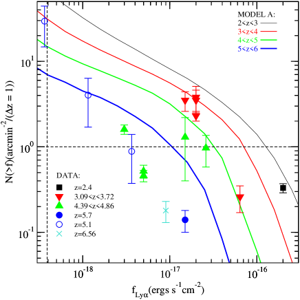
Figure 1: The predicted number of Ly-$\alpha$ emitters in model A, compared to the observational data compiled in Table 2. The observational data are divided into different redshift ranges, as indicated by the lower key, and we have plotted only datapoints based on more than one galaxy. Model predictions are shown by lines, as indicated by the upper key. The thickness of the lines increases with redshift. The vertical and horizontal dashed lines indicate the sensitivity limits in flux and number density for a reference MUSE observation (see text).

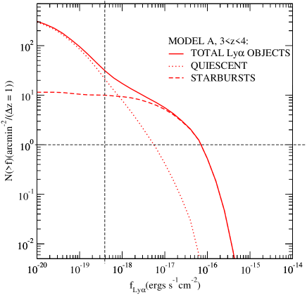
Figure 2: The predicted number counts of Ly-$\alpha$ emitters in model A, in the redshift range $z=3-4$. The contributions from quiescent star forming galaxies and ongoing starbursts are plotted separately, as indicated in the key. The vertical and horizontal dashed lines are the same as in Fig. 1.

We explore the impact on the abundances of Ly-$\alpha$ emitters of varying the redshift at which the Universe was reionized, $z_{\rm reion}$, which is still poorly constrained.

(1)	(2)	(3)	(4)	(5)	(6)	(7)	(8)	(9)	(10)	(11)
z	$\Delta z$	$f$	$\frac{d^{2}N}{dzd\Omega}(>f)$	$\Delta\left(\frac{d^{2}N}{dzd\Omega}\right)$	Nobj	Area	Fcorr	method	confirmation	ref.
$2.42$	$0.14$	$20$	$0.33$	$0.04$	$58$	$1200$	$0.65$	NBF	EW/colour	Sti01
$3.09$	$0.07$	$2$	$2.3$∗	$0.3$	$12$∗	$78$	$0.94$	NBF	EW/colour	Ste00
$3.13$	$0.04$	$2$	$3.8$	$1.3$	$8$	$49$	$0.7$	NBF	spec on 10	K00
$3.43$	$0.06$	$1.5$	$3.5$	$0.9$	$16$	$75$	$0.87$	NBF	spec on 15	H98
$3.72$	$0.23$	$6.4$	$0.26$	$0.09$	$8$	$130$	$0.35$	NBF	colours	F03
$4.39$	$0.07$	$2.6$	$0.97$	$0.11$	$75$	$1100$	$0.33$	NBF	spec on 3	R00
$4.54$	$0.06$	$1.5$	$1.3$	$0.9$	$2$	24	$0.67$	NBF	spec on 3	H98
$4.79$	$0.08$	$0.5$	$0.46$	$0.07$	$41$	$1100$	$0.8$	NBF	$-$	S04
$4.86$	$0.06$	$0.5$	$0.52$	$0.09$	$34$	$1100$	$0.8$	NBF	spec on 5	S03
$4.86$	$0.06$	$0.3$	$1.6$	$0.2$	$52$	$540$	$0.6$	NBF	colours	O03
$5.1$	$1.0$	$0.012$∗∗	$48$∗∗	$48$	$1$	$0.02$∗∗	$-$	LS	$-$	Sa04
$``$	$``$	$0.037$∗∗	$30$∗∗	$15$	$4$	$0.14$∗∗	$-$	$``$	$-$	“
$``$	$``$	$0.12$∗∗	$4.0$∗∗	$2.3$	$3$	$0.75$∗∗	$-$	$``$	$-$	“
$``$	$``$	$0.37$∗∗	$0.89$∗∗	$0.51$	$3$	$3.4$∗∗	$-$	$``$	$-$	“
$``$	$``$	$1.2$∗∗	$0.14$∗∗	$0.14$	$1$	$7.5$∗∗	$-$	$``$	$-$	“
$5.3$	$1.0$	$2?$	$2.3$	$1.0$	$5$	$2.2$	$-$	LS	$-$	D01
$5.7$	$0.13$	$1.5$	$0.14$	$0.04$	$13$	$710$	$0.75$	NBF	spec on 4	R03
$6.56$	$0.10$	$0.6$∗∗	$20$∗∗	$20$	$1$	$0.46$∗∗	$1$	NBF	spec on 1	H02
$6.56$	$0.11$	$0.9$	$0.18$	$0.05$	$16$	$810$	$0.22$	NBF	spec on 9	K03

Table 2: Data Compilation. The data are divided into unit redshift intervals: the following symbols are used to denote data from each redshift interval in the figures ($\blacksquare$ :[$z<3$], $\blacktriangledown$ :[$3<z<4$], $\blacktriangle$ :[$4<z<5$], $\circ$:[$z=5.1$], $\bullet$:[$5<z<6$], X:[$6<z<7$]). Col.1: redshift; Col.2: redshift interval; Col.3: Ly-$\alpha$ flux (in $10^{-17}{\rm ergs\,cm}^{-2}{\rm s}^{-1}$); Col.4: cumulative counts per unit solid angle per unit redshift (in ${\rm arcmin}^{-2}$); Col.5: Poisson error on counts (in ${\rm arcmin}^{-2}$); Col.6: number of Ly-$\alpha$ emitters; Col.7: area of survey (in ${\rm arcmin}^{2}$); Col.8: factor applied to correct for contamination by low-z interlopers; Col.9: method (NBF=narrow band filter, LS=long-slit spectroscopy); Col.10: method used to reject or correct for low-z interlopers (EW=equivalent width, spec on N = follow-up spectroscopy of N objects); Col.11: reference (D01: Dawson et al. 2001; F03: Fujita et al. 2003; H98: Hu et al. 1998; H02: Hu et al. 2002; K03: Kodaira et al. 2003; K00: Kudritzki et al. 2000; O03: Ouchi et al. 2003; R00: Rhoads et al. 2000; R03: Rhoads et al. 2003; Sa04: Santos et al. 2004; S03: Shimasaku et al. 2003; S04: Shimasaku et al. 2004; Ste00: Steidel et al. 2000; Sti01: Stiavelli et al. 2001)

^∗ corrected for factor 6 overdensity   ^∗∗ corrected for gravitational lensing

We examine the consequences of making three choices: (i) $z_{\rm reion}=10$, (ii) $z_{\rm reion}=20$ and (iii) $z_{\rm reion}=6$. The first two values are consistent with the optical depth to last scattering suggested by the WMAP measurement of the correlation between microwave background temperature and polarization [Kogut et al. 2003]. The latter value is suggested by the detection of a Gunn-Peterson trough in the spectrum of a $z=6.28$ quasar by Becker et al. (2001). In the model, gas is prevented from cooling in haloes with circular velocities below $60{\rm kms}^{-1}$ for redshifts $z<z_{\rm reion}$. The models that we consider are listed in Table 1. Models A-E reproduce the observed luminosity function for the local galaxy population (e.g. Baugh et al. 2004). Finally, we also consider the effect on the counts of Ly-$\alpha$ emitters of varying the cosmological density parameter, $\Omega$ (models F and G). Note that we have not attempted to vary any other parameters of the GALFORM model in these two cases to force the model to reproduce the local galaxy luminosity function.

3 The observational data and model predictions

We list in Table 2 a compilation of published observational data on number counts of Ly-$\alpha$ emitters at different observed line fluxes and redshifts from “blank field” surveys that we will compare against our model predictions. Note that some of the quantities listed in Table 2 are derived from the information given in the original sources, so we present this compilation in order to facilitate future comparisons between data and model predictions by other authors. We do not include data from surveys targetted around high-z objects such as quasars (e.g. Fynbo et al. 2001), since in this case the number density of Ly-$\alpha$ emitters may be biased by an unknown factor. A few of the surveys used spectroscopy to directly search for Ly-$\alpha$ emitters. However, most used narrow-band imaging to identify objects having a strong emission line at the wavelength corresponding to Ly-$\alpha$ at a particular redshift. Samples of objects obtained in this way are generally contaminated by lower redshift galaxies for which some other emission line (e.g. $[OII]3737$, $[OIII]5007$, $H\alpha$) happens to fall at the same wavelength. This contamination is typically estimated and removed using the equivalent width of the emission line and/or broad-band colours, or from follow-up spectroscopy on a subsample of the objects. The methods used in the different surveys are indicated in the table.

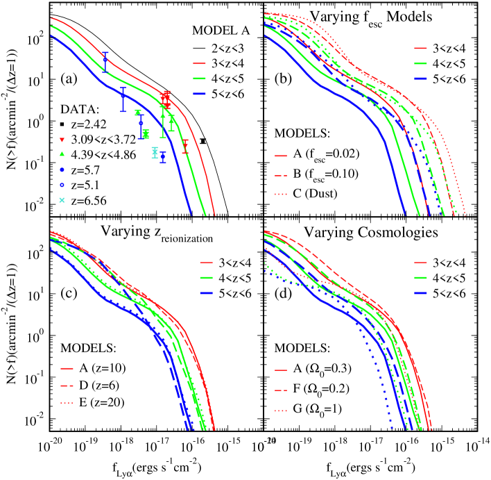
Figure 3: The predicted counts of Ly-$\alpha$ emitting galaxies, plotted in different redshift intervals, as indicated by the key. (a) Shows the predictions for model A; a subset of these are reproduced in each panel for reference. The data from Fig. 1 are also plotted here using the same symbols as before. The remaining panels show the impact on the predictions of changing different aspects of the model: (b) Varying the escape fraction or using a dust model. (c) Varying the redshift of reionization. (d) Varying the cosmological density parameter.

The observational data are plotted in Fig. 1, with different symbols indicating data from a given unit redshift range. The predictions of our fiducial model, A from Table 1, are shown by the solid lines in Fig. 1. The escape fraction $f_{\rm esc}$ was set to give a reasonable match to the observed number counts at $z\sim 3$. This simple model, in which the escape fraction is independent of redshift and galaxy properties, does a surprisingly good job of matching the observed counts at different redshifts.

The separate contributions to the counts of Ly-$\alpha$ emitters from galaxies that are forming stars quiescently and from ongoing starbursts (which in our model are triggered by galaxy mergers) are shown in Fig. 2 for model A over the redshift interval $z=3-4$. Quiescently star forming galaxies dominate at fainter fluxes, whereas starbursts account for the brighter Ly-$\alpha$ sources. This is largely due to the flat IMF assumed in starbursts, which typically yields ten times the number of Lyman continuum photons for a given amount of star formation, compared with the Kennicutt (1998) IMF that we adopt for quiescent star formation.

In Fig. 3, we present the predicted counts of Ly-$\alpha$ emitters as a function of redshift for the different GALFORM models listed in Table 1. The results for model A, our fiducial model, are reproduced for reference in each panel. In Fig. 3(b) we show the effect of increasing the escape fraction $f_{\rm esc}$ by a factor of 5. Fig. 3(b) also shows that assuming a fixed escape fraction $f_{\rm esc}=0.1$ produces similar number counts to a model in which the Ly-$\alpha$ photons are absorbed by diffuse dust without resonant scattering, as might occur in a galactic wind. Fig. 3(c) shows the impact on the predicted counts of varying the redshift at which the universe is reionized. For model D, with $z_{\rm reion}=6$, the number of faint Ly-$\alpha$ sources changes substantially for $5<z<6$ and $4<z<5$, compared with the cases where $z_{\rm reion}\geq 10$. This is because in model D gas is still able to cool in low mass haloes (i.e. with circular velocities below $60{\rm kms}^{-1}$) up to $z=6$, and is available to form stars and thus generate Lyman continuum photons. Finally, Fig. 3(d) illustrates the effect of changing the cosmological density parameter whilst retaining a flat universe. The changes in the model predictions in this case primarily reflect the change in the normalisation of density fluctuations, as specified by $\sigma_{8}$ in Table 1, which is adjusted to reproduce the local abundance of rich clusters when the density parameter is varied.

4 Discussion and conclusions

The conclusion of this first study to look at the predictions of hierarchical models for the number of Ly-$\alpha$ emitters is that simple models do remarkably well at reproducing the observed counts. Assuming that typically just 2 % of the Ly-$\alpha$ photons escape from high-z galaxies, a value chosen to match the observed counts at $z\sim 3$, is sufficient to give a reasonable match to the observed counts at faint fluxes over the redshift interval $2<z<6$.

This study demonstrates the capability of semi-analytical modelling to make predictions that can serve as an input into the design of new instruments. The Multi-Unit Spectroscopic Explorer (MUSE) [Bacon et al. 2004] has been proposed to ESO as a second-generation instrument for the Very Large Telescope. MUSE will be able to identify Ly-$\alpha$ emitters over a redshift interval $2.8<z<6.7$ over a field of view of 1 arcmin². An exposure of 80 hours will reach a 5 $\sigma$ sensitivity of $3.9\times 10^{-19}$ erg/s/cm². We predict that MUSE will be able to detect a large number of such objects at this flux limit: around 70-400 per arcmin² (see the final column of Table 1). Observations with MUSE will be able to exclude some of the models we have considered, and therefore remove some of the uncertainties in our modelling of Ly-$\alpha$ emission. More importantly, such observations will provide a critical test of our ideas about star formation in objects at high redshifts.

References

- [Ahn 2004] Ahn, S.-H., 2004, ApJ, 601, L25
- [Bacon et al. 2004] Bacon R., et al. 2004, SPIE
- [Baugh et al. 1998] Baugh C.M., Cole S., Frenk C.S., Lacey C.G., 1998, ApJ, 498, 504
- [Baugh et al. 2004] Baugh C.M., Lacey C.G., Frenk C.S., Granato G.L., Silva L., Bressan A., Benson A.J., Cole S., 2004, MNRAS, submitted. (astro-ph/0406069).
- [Becker et al. 2001] Becker R.H., et al. 2001, AJ, 122, 2850.
- [Benson et al. 2003] Benson A.J., Frenk C.S. Baugh C.M., Cole S., Lacey C.G., 2003, ApJ, 599, 38
- [Cole et al. 1994] Cole S., Aragon-Salamanca A., Frenk C.S., Navarro J.F., Zepf S., 1994, MNRAS, 271, 781.
- [Cole et al. 2000] Cole S., Lacey C.G., Baugh C.M., Frenk C.S., 2000, MNRAS, 319, 168.
- [CH98] Cowie L.L., Hu E.M., 1998, AJ, 115, 1319.
- [D01] Dawson S., Stern D., Bunker A.J., Spinrad H., Dey A. 2001, AJ, 122, 598. (D01)
- [Eke et al. 1996] Eke V.R., Cole S., Frenk C.S., 1996, MNRAS, 282, 263
- [F03] Fujita S.S., et al., 2003, AJ, 125, 13.(F03)
- [Fynbo et al. 2001] Fynbo J.U., Moller P., Thomsen B., 2001, A&A, 374, 443.
- [Haiman & Spaans 1999] Haiman Z., Spaans M., 1999, ApJ, 518, 138.
- [Hatton et al. 2003] Hatton S., Devriendt J.E.G., Ninin S., Bouchet F.R., Guiderdoni B., Vibert D., 2003, MNRAS, 343, 75.
- [Hu & McMahon 1996] Hu E.M., McMahon R.G., 1996, Nature, 382, 231.
- [H98] Hu E.M., Cowie L.L., McMahon R.G., 1998, ApJ, 502, L99. (H98)
- [H02] Hu E.M., Cowie L.L., McMahon R.G., Capak P., Iwamuro F., Kneib J.-P., Maihara T., Motohara K. 2002, ApJ, 568, L75. (H02)
- [Kauffmann et al. 1994] Kauffmann G., Guiderdoni B., White S.D.M., 1994, MNRAS, 267, 981.
- [Kennicutt 1998] Kennicutt R.C., 1998, ApJ, 498, 541.
- [K03] Kodaira K., et al. 2003, PASJ, 55, L17. (K03)
- [Kogut et al. 2003] Kogut A., et al. (the WMAP team), 2003, ApJS, 148, 161.
- [K00] Kudritzki R.-P., et al. 2000, ApJ, 536, 19. (K00)
- [Kunth et al. 1998] Kunth, D., Mas-Hesse, J.M., Terlevich, E., Terlevich, R., Lequeux, J., Fall, S.M., 1998, A&A, 334, 11
- [Osterbrock 1989] Osterbrock D.E., 1989, Astrophysics of Gaseous Nebulae
- [O03] Ouchi M.,et al. 2003, ApJ, 582, 60. (O03)
- [Pettini et al. 2001] Pettini M., Steidel C.C., Adelberger K.L., Dickinson M., Giavalisco M., 2001, ApJ, 528, 96.
- [R00] Rhoads J.E., Malhotra S., Dey A., Stern D., Spinrad H., Jannuzi B.T. 2000, ApJ, 545, L85. (R00)
- [R03] Rhoads J.E., et al. 2003, AJ, 125, 1006. (R03)
- [Sa04] Santos M.R., Ellis R.S., Kneib J.P., Richard J., Kuijken K., 2004, ApJ, 606, 683. (Sa04)
- [S03] Shimasaku K.,et al. 2003, ApJ, 586, L111. (S03)
- [S04] Shimasaku, K., et al. 2004, ApJ, 605, L93. (S04)
- [Somerville & Primack 1999] Somerville R.S. Primack J.R., 1999, MNRAS, 310, 1087.
- [Steidel et al. 1996] Steidel C.C, Giavalisco M., Dickinson M., Adelberger K.L., 1996, AJ, 112, 352.
- [Ste00] Steidel C.C., Adelberger K.L., Shapley A.E., Pettini M., Dickinson M., Giavalisco M., 2000, ApJ, 532, 170. (Ste00)
- [Sti01] Stiavelli M., Scarlata C., Panagia N., Treu T., Bertin G., Bertola F. 2001, ApJ, 561, L37. (Sti01)