Search for very high energy gamma-rays from WIMP annihilations near the Sun with the Milagro Detector

Abstract

The neutralino, the lightest stable supersymmetric particle, is a strong theoretical candidate for the missing astronomical “dark matter”. A profusion of such neutralinos can accumulate near the Sun when they lose energy upon scattering and are gravitationally captured. Pair-annihilations of those neutralinos may produce very high energy (VHE, above $100\ GeV$) gamma-rays.

Milagro is an air shower array which uses the water Cherenkov technique to detect extensive air showers and is capable of observing VHE gamma-rays from the direction of the Sun with an angular resolution of $0.75^{\circ}$. Analysis of Milagro data with an exposure to the Sun of 1165 hours presents the first attempt to detect TeV gamma-rays produced by annihilating neutralinos captured by the Solar system and shows no statistically significant signal. Resulting limits that can be set on gamma-ray flux due to near-Solar neutralino annihilations and on neutralino cross-section are presented.

I Introduction

There is very strong evidence that the Universe, and the galaxies in particular, are full of non-baryonic “dark matter” (see, for example, Rubin ; netterfield ; halverson ; stompor ; perlmutter ; riess ; spergel ). One candidate for this dark matter is the neutralino ($\chi$) — a weakly interacting massive particle (WIMP) predicted by super-symmetric theories Haber ; Jungman . Experimental tests for this possibility include direct searches with extremely sensitive devices which can detect energy deposited by a neutralino when it elastically scatters off a nucleus and indirect searches which look for products of neutralino-neutralino annihilations.

The Italian/Chinese collaboration (DAMA) employs an ionization bolometer and has reported an observation which they interpret as consistent with the annual modulation predicted if WIMPs exist DAMA . However, there are possible modulating systematic errors. The CDMS experiment detects phonon vibrations of the crystal lattice caused by the neutralino-nucleon scattering in the detector volume and has obtained data that appear to exclude most of the DAMA-allowed region CDMS . They reach a spin-independent WIMP-nucleon cross-section limit around $2\cdot 10^{-42}\ cm^{2}$ in the mass range $20-100\ GeV$. Edelweiss, which utilizes both phonon and ionization bolometers, has also released results that significantly cut into the DAMA allowed region Edelweiss .

Indirect searches look for decay products from neutralino annihilations coming from regions with enhanced neutralino densities. Searches vary by the regions explored (such as the Galactic center or the Sun) and by the decay products being detected. Unlike direct searches, interpretation of these experiments requires assumptions about astrophysical parameters which give rise to the neutralino annihilation distribution in the region being studied. They also depend on cross-sections and branching ratios, both of which are supersymmetry-model dependent.

An increased density of neutralinos may exist in the vicinity of the Galactic center or the Sun PressSpergel . This could have arisen in the initial formation of these objects. Also, neutralinos entering the Solar system (or the Galaxy) may lose energy via elastic scattering with ordinary matter and become gravitationally trapped. Due to the capture and repeated scatterings, there would be a near-solar (or Galactic-center) enhancement in the neutralino density. Such a local neutralino build-up may provide a detectable flux of annihilation products. Examples of indirect searches are those by the Kamiokande and SuperKamiokande underground neutrino detectors that have set limits on solar and terrestrial neutralino-induced muon fluxes Mori ; SuperK2001 . Such searches are helped by the ability of neutrinos to escape from their production region and by the typically large predicted yield, but are hindered by the small detection probability.

Another possible method for detecting dark matter particles is from their annihilation into $\gamma$-rays. The Minimal Supersymmetric extension of the Standard Model (MSSM) predicts that the gamma rays emerging from $\chi\chi\rightarrow\gamma\gamma$ and $\chi\chi\rightarrow Z\gamma$ neutralino annihilation modes will give distinct monochromatic signals in the energy range between $100\ GeV$ and $10\ TeV$, depending on the neutralino mass. An additional “continuum” spectrum signal of photons will be produced by the decay of secondaries produced in the non-photonic annihilation modes. However, past and present high energy gamma-ray experiments, such as EGRET and the Whipple atmospheric Cherenkov Telescope, lack the sensitivity to detect annihilation $\gamma$-line fluxes predicted for many allowed supersymmetric models and Milky Way halo profiles. The next generation ground-based and satellite gamma-ray experiments, such as VERITAS and GLAST, will allow exploration of portions of the MSSM parameter space, assuming that the dark matter density is peaked at the galactic center Bergstrom3 .

The Milagro $\gamma$-ray observatory, which has been taking data since 1999, is sensitive to cosmic gamma rays at energies around 1 TeV and is capable of continuously monitoring the overhead sky with angular resolution of $0.75^{\circ}$. In this paper, we present the results of a search for a TeV gamma-ray signal from the vicinity of the Sun (1-2 solar radii) with Milagro.

II Milagro detector

The Milagro Extensive-Air Shower Array is located at $35.88^{\circ}$ North latitude and $106.68^{\circ}$ West longitude in the Jemez Mountains near Los Alamos, New Mexico. At an altitude of $2630\ m$ above the sea level, its atmospheric overburden is about $750\ g/cm^{2}$. The Milagro detector, commissioned in June of 1999, records about 1700 extensive air shower events per second and is sensitive to gamma-showers with energies above $\sim\!\!100\ GeV$. The detector consists of a 21 kiloton water-filled pond instrumented with two layers of photo-multiplier tubes (PMTs). These PMTs detect Cherenkov light produced by secondary shower particles which enter the pond. The top(bottom) layer has 450 (273) PMTs arranged on a $2.8\times 2.8\ m$ grid, $1.4\ (6)\ m$ below the water surface.

The direction of each shower is determined as the normal of the plane fitted to the PMTs’ times using an iterative weighted $\chi^{2}$-method which rejects outliers. The weights for the $\chi^{2}$-fit are prescribed based on the PMT signal strength. The angular resolution of the array is estimated to be $0.75^{\circ}$.

Extensive air showers produced by cosmic rays are the primary source of triggers in the experiment. These showers are likely to contain hadrons that reach the ground level and produce hadronic cascades in the detector, or muons that penetrate to the bottom layer, and will thus illuminate a relatively small number of neighboring PMTs in that layer. Photon induced showers, on the other hand, generally will produce rather smooth light intensity distributions. Based on this observation, a technique for identification of gamma versus hadron initiated showers has been formulated MilagroCrab and according to computer simulations can correctly select about 90% of hadron initiated showers and about 50% of photon induced ones.

The fluctuations in the shower development, small size of the detector and fluctuations in its response make energy determination on the event-by-event basis difficult. The absolute energy scale can be determined by examining the displacement of the shadow of the Moon due to the Earth’s magnetic field MilagroMoon . For a more detailed description of the detector itself and reconstruction techniques used, see references milagritoNIM ; milagroNIM ; MilagroCrab .

III Data analysis.

While it is difficult to tell the difference between cosmic-ray and gamma-ray initiated showers, a gamma-ray signal can be detected as an excess of events from the direction of the Sun above that expected from the cosmic-ray background. The data analysis procedure thus entails determining the average expected background signal $N_{on}^{b}$, counting the number of events from the direction of the Sun $N_{on}$ and determining the statistical significance of any excess found.

For each position of the Sun $N_{on}^{b}$ is found using event rates from the same local region of the sky at a time when the Sun is not present using the technique described in RomanPaper . This method is based on isotropy of the cosmic-ray background and the assumption of short time scale detector stability. It allows exclusion of known sources from background estimation and correct restoration of the number of excess events to be used for flux measurement.

The statistic $U$ chosen to test for an excess is:

$$U=\frac{N_{on}-N_{on}^{b}}{\sqrt{\alpha N_{on}+N_{on}^{b}}}$$ (1)

where $\alpha$ is the relative exposure ratio of the “ on-source” region to the “off-source” one. For detailed discussion on how to deal with varying $\alpha$ see RomanPaper . In the absence of a source, $U$ approximately obeys a Gaussian distribution with zero mean and unit variance. If a source is present, $U$ will still have an approximately Gaussian distribution with unit dispersion but with a shifted mean.

For the current search we define at the outset the critical value of the statistic $U$ as $u_{c}=5$ (which approximately corresponds to the level of significance of $2.9\cdot 10^{-7}$). If no excess from the vicinity of the Sun is found, we construct a limit on the source strength as a strength which, if present, would have given us a detectable signal ($u>5$) with $97.7\%$ ($2\sigma$) probability exclusionPaper . In addition, following the more standard procedure eadie , assuming that the source exists, a $90\%$ one-sided confidence interval on its strength is also calculated.

Given the detector response to particles of different types and assumed source features, it is possible to predict the number of events $N_{k}$ to be observed due to the source.

$$N_{k}=\int F(k,E)S(k,\Theta)T(\Theta)\left[\int_{\tilde{\Theta}\in\tilde{\Omega}}A_{k}(E,\Theta,\tilde{\Theta})\,d\tilde{\Theta}\right]\,dE\,d\Theta$$ (2)

where $F(k,E)$ is the number of particles of type $k$ with energy $E$ emitted by the source per unit area per unit time, $S(k,\Theta)$ describes the known geometrical shape of the source and is assumed to be energy independent, $T(\Theta)$ is the time during which the source is located in local direction $\Theta$ and $\tilde{\Theta}$ is the direction of the particle arrival as output by the reconstruction algorithm. The function $A_{k}(E,\Theta,\tilde{\Theta})$ is known as the “effective area” of the detector and can be integrated over $\tilde{\Theta}$ prior to data processing for selected configuration of $\tilde{\Omega}$. Therefore, after integration over $\Theta$, the number of events due to particles of type $k$ to be observed from a region $\tilde{\Omega}$ is:

$$N_{k}=\int F(k,E)A_{k}^{T}(E)\,dE$$ (3)

The integrated effective area $A_{k}^{T}(E)$ is obtained during the data processing from Monte Carlo generated effective area $A_{k}(E,\Theta,\tilde{\Theta})$. By counting the number of excess events in an observation bin $N_{\gamma}=N_{on}-N_{on}^{b}$, it is thus possible to deduce some properties of the source function $F(\gamma,E)$.

IV Effect of the Sun shadow

The gamma ray signal from neutralino annihilations near the Sun should appear as an excess number of events from the direction of the Sun over the expected cosmic-ray background. The interpretation of any observed signal, however, is not an easy problem. Largely, this is due to the fact that the cosmic-ray background is not expected to be uniform; the Sun absorbs the cosmic rays impinging on it and forms a cosmic-ray shadow. The situation is complicated by the magnetic fields of the Earth and the Sun. Due to bending of charged-particle trajectories in magnetic fields, the Sun’s shadow in the TeV range of particle energies will be smeared and shifted from the geometrical position of the Sun. On the other hand, in the presence of strong Solar magnetic fields, lower energy particles cannot reach the surface of the Sun and are reflected from it. Such particles are not removed from the interplanetary medium and, since the cosmic rays are isotropically incident on the Sun, may not even form a cosmic-ray shadow. In addition, the Solar magnetic field varies with time, which will smear the shadow in a long-exposure observation. Therefore, it is difficult to ascertain the exact shape of the cosmic-ray shadow at the Sun’s position and deduce an excess above it.

Nevertheless, the effect of the Earth’s magnetic field and the Solar wind can be studied by observing the shadow of the Moon during the solar day. The effect of the geomagnetic field on the shadows of the Sun and the Moon should be very similar since the Sun and the Moon cover similar size regions on the celestial sphere and traverse similar paths on the local sky in one year of observation. In addition, the Earth’s magnetic field at the Moon distance is already so small that any additional deflection beyond the Moon distance by this field of particles originating from the Sun can be neglected.

A deficit of events due to such a shadow could be filled by a signal from neutralinos which would remain undetected when the excess is searched for. Since the shadow depth is unknown, when performing a search for evidence of a positive excess we are forced to assume the absence of the shadow. On the other hand, for setting a conservative limit on the photon flux we use the maximum possible depth of the shadow.

The deficit of events from the direction of the Sun can not be greater than that produced by the Moon because as mentioned above the additional Solar magnetic field can only decrease its shadow relative to the Moon. To be conservative in setting the gamma-ray flux limit, the strongest event deficit produced by the Moon in $5^{\circ}$ radius from its position, corrected for relative Sun/Moon exposure, is used as a correction for the possible presence of a shadow of the Sun.

V Results

V.1 Outcome of the observation

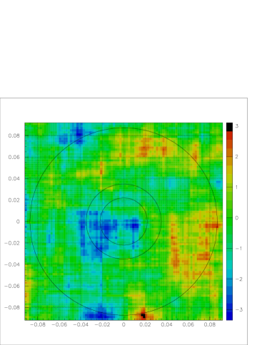
(a)

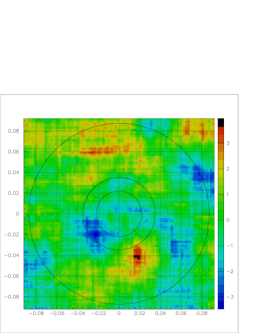
(b)

(c)

(d)

Figure 1: The maps of statistical significance of the number of excess events from the regions of the sky around the daytime Moon (1(a)) and the Sun (1(b)) and the corresponding source exposure as function of zenith angle in hours per degree (1(c),1(d)). The color code is the value of $U$ (see equation (1)). The Moon shadow is much less significant than that reported in MilagroMoon because of $\gamma$-selection and other cuts used in the present analysis. The maps are made using azimuthal equal-area projection in polar case centered on the corresponding Celestial object. Contours represent loci of distance $1.26^{\circ}$, $2.0^{\circ}$ and $5.0^{\circ}$ from the Celestial object.

The data used in this work was chosen to satisfy the following conditions: online reconstruction between the 19th of July 2000 and the 10th of September 2001, the number of PMTs required for a shower to trigger the detector greater than $60$, the number of PMTs used in the angular reconstruction greater than $20$, zenith angles smaller than $45$ degrees, and passing the gamma/hadron separation cut MilagroCrab . The start and end dates correspond respectively to introduction of the hadron separation parameter into the online reconstruction code and detector turn-off for scheduled repairs. Several data runs were removed from the dataset which included calibration runs and the data recorded when there were online DAQ problems.

For the solar region analysis, $\pm 5^{\circ}$ regions around the Moon and the Crab nebula were vetoed from the data set as they present known sources of anisotropy to the cosmic-ray background.

Photons produced in the Sun will be absorbed, whereas the distribution of neutralino annihilations outside is a rapidly falling function of distance from the Sun. Therefore, we believe that the gamma-ray signal is produced mostly between 1 and 2 solar radii and treat the gamma-ray source as circle of $0.5^{\circ}$ radius. It has been shown LazarPhD that the optimal bin size is a slow function of the source size and for estimated $0.75^{\circ}$ angular resolution of the detector, the optimal “on-source” bin is a circular one with the radius of $1.26^{\circ}$ centered on the Sun.

Overall, $1164.7$ hours of exposure to the Sun is obtained in the data set. The total number of events observed in the “on-source” bin is $N_{on}=137211$ while $N_{on}^{b}=137728$ events is expected based on the “off-source” exposure, leading to the value of the test statistic $U$ of $-1.35$ (see figure 1). Therefore, the null hypothesis of the absence of gamma-ray emission from the Sun can not be rejected and a limit on the possible $\gamma$-ray flux from the solar region is obtained.

Overall, 423.5 hours of exposure to the Moon during the day time is obtained in this data set after $\pm 5^{\circ}$ regions around the Sun and the Crab nebula were vetoed. The largest deficit observed in the sky map centered on the geometrical position of the Moon is $-3.3$ corresponding to $-766$ events (see figure 1). The exposure on the Sun is $2.75$ times greater than that on the Moon during solar day, leading to estimated maximal deficit in the Sun’s direction as: $-766\cdot 2.75=-2107$.

Hence, using the criteria outlined in section III we conclude that the number of excess events due to a possible Solar source of VHE photons does not exceed $N_{exclude}=4791$. It is this number which is used to construct the exclusion region on gamma-ray flux strength from the Solar region (equation 3).

The $90\%$ one-sided confidence interval on the average number of excess events $N_{confidence}$ assuming that gamma-ray emission from the Sun exists constructed in a standard way eadie is $N_{confidence}=2081$. It is this number which would allow estimation of the gamma-ray flux strength from the Solar region if it were known that such gamma-ray emission exists (equation 3).

V.2 Limit on the photon flux due to neutralino annihilations

Figure 2: Integrated effective area $A_{k}^{T}$ as a function of photon (solid) and proton (dashed) energy (see equation (3)) for the circular $1.26^{\circ}$ bin centered on the Sun for the trigger condition and cuts used in this analysis.

Figure 3: The values of ($F_{\delta}$,$F_{c}$) below the lines are allowed for corresponding neutralino masses.

$m_{\chi}\ (TeV)$	$\Delta\ (cm^{2}s)$	$\Sigma\ (cm^{2}s)$
0.1	$1.055\times 10^{11}$	$0.000$
0.2	$8.772\times 10^{11}$	$4.969\times 10^{7}$
0.5	$6.070\times 10^{12}$	$2.634\times 10^{9}$
1.0	$3.389\times 10^{13}$	$2.127\times 10^{10}$
2.0	$1.600\times 10^{14}$	$1.280\times 10^{11}$
5.0	$5.942\times 10^{14}$	$1.208\times 10^{12}$
10.0	$1.608\times 10^{15}$	$5.575\times 10^{12}$
20.0	$3.684\times 10^{15}$	$2.136\times 10^{13}$
50.0	$8.030\times 10^{15}$	$1.035\times 10^{14}$

Table 1: Coefficients of the flux limit calculation (see equation (5)).

$m_{\chi}\ (TeV)$	$F_{\delta}<\ (cm^{-2}s^{-1})$	$F_{c}<\ (cm^{-2}s^{-1})$
0.1	$4.54\times 10^{-8}$	—
0.2	$5.46\times 10^{-9}$	$9.64\times 10^{-5}$
0.5	$7.89\times 10^{-10}$	$1.82\times 10^{-6}$
1.0	$1.41\times 10^{-10}$	$2.25\times 10^{-7}$
2.0	$2.99\times 10^{-11}$	$3.74\times 10^{-8}$
5.0	$8.06\times 10^{-12}$	$3.97\times 10^{-9}$
10.0	$2.98\times 10^{-12}$	$8.59\times 10^{-10}$
20.0	$1.30\times 10^{-12}$	$2.24\times 10^{-10}$
50.0	$5.97\times 10^{-13}$	$4.63\times 10^{-11}$

Table 2: The limit on the flux parameters $(F_{\delta},F_{c})$ corresponding to the significance $2.9\cdot 10^{-7}$ and the power of the test of $97.7\%$. For the $90\%$ one-sided confidence interval multiply these limits by $0.4344$.

Because the two close direct-production spectral lines can not be resolved by the Milagro detector, the differential photon flux due to neutralino annihilations is assumed to have the form (see Bergstrom3 ):

$$\frac{dF(E_{\gamma})}{dE_{\gamma}}=F_{\delta}\delta(E_{\gamma}-m_{\chi})+\frac{F_{c}}{m_{\chi}}\cdot\frac{\Big{(}\frac{E_{\gamma}}{m_{\chi}}\Big{)}^{-3/2}e^{-7.8E/m_{\chi}}}{\int_{0.01}^{1}x^{-3/2}e^{-7.8x}dx}$$ (4)

where $F_{\delta}$ is the integral flux due to a $\delta$-function-like photon annihilation channel and $F_{c}$ is the integral flux of photons with energies greater than $0.01\cdot m_{\chi}$ due to continuum photon spectrum annihilation channel of neutralinos with mass $m_{\chi}$. Here, the normalization of the continuum photon spectrum has been written out explicitly.

Using this expression for the flux with the integrated effective area of the detector, we find a relationship between the number of observed events $N_{\gamma}$ and the integral flux parameters $F_{\delta}$ and $F_{c}$ in the form:

$$F_{\delta}\Delta+F_{c}\Sigma=N_{\gamma}$$ (5)

The values of coefficients $\Delta$ and $\Sigma$ (see table 1) are obtained by substituting the expression for flux (4) and the integrated effective area (figure 2) into the formula for the number of expected events (3). Note, that depending on $m_{\chi}$ the integral in (3) may extend below the $0.01m_{\chi}$ normalization.

The figure 3 presents the curves demarcating the allowed and excluded regions in the photon flux parameter space $(F_{\delta},F_{c})$ corresponding to the significance $2.9\cdot 10^{-7}$ and the power of the test of $97.7\%$ obtained by setting $N_{\gamma}=N_{exclude}$ which have a form of straight lines in the $(F_{\delta},F_{c})$ plane. Because there is only one equation (eq. (5)) constraining two parameters, table 2 provides the most conservative limits on each of $F_{\delta}$ and $F_{c}$ when the contribution from the other is set to zero.

For the depiction of the one-sided $90\%$ confidence interval in the $(F_{\delta},F_{c})$ plane, both axes in the figure 3 should be rescaled by $N_{exclude}/N_{confidence}=0.4344$.

Figure 3 is the derived limit on the values of the parameters of the gamma-ray emission model (equation (4)) due to near solar WIMP annihilation and is independent of the models of their distribution in the Milky Way galaxy and the Solar system.

V.3 Neutralino limits

$m_{\chi},\ (TeV)$	$I(m_{\chi})\times\frac{10^{-43}cm^{2}}{\sigma_{p\chi}}\frac{0.3GeV/cm^{3}}{\rho_{0}},\ (s^{-1})$
$0.1$	$1.65\times 10^{18}$
$0.2$	$4.17\times 10^{17}$
$0.5$	$6.72\times 10^{16}$
$1.0$	$1.68\times 10^{16}$
$2.0$	$4.22\times 10^{15}$
$5.0$	$6.72\times 10^{14}$
$10.0$	$1.69\times 10^{14}$
$20.0$	$4.22\times 10^{13}$
$50.0$	$6.75\times 10^{12}$

Table 3: Capture rate $I(m_{\chi})$ as a function of neutralino mass $m_{\chi}$ obtained in a three-dimensional calculation LazarPhD . The normalizations of $\sigma_{p\chi}$ and $\rho_{0}$ are typically used numbers.

$m_{\chi}\ (TeV)$	$\left(J/I\right)\frac{\sigma_{p\chi}}{10^{-43}cm^{2}}\frac{\rho_{0}}{0.3GeV/cm^{3}}b_{\gamma}^{c}f_{out}<$	$\left(J/I\right)\frac{\sigma_{p\chi}}{10^{-43}cm^{2}}\frac{\rho_{0}}{0.3GeV/cm^{3}}b_{\gamma}^{\delta}f_{out}<$
0.1	—	$155$
0.2	$1.30\times 10^{6}$	$73.7$
0.5	$1.52\times 10^{5}$	$66.1$
1.0	$7.54\times 10^{4}$	$47.3$
2.0	$4.99\times 10^{4}$	$39.9$
5.0	$3.32\times 10^{4}$	$67.5$
10.0	$2.86\times 10^{4}$	$99.2$
20.0	$2.99\times 10^{4}$	$173$
50.0	$3.86\times 10^{4}$	$497$

Table 4: The limits on $J(m_{\chi})/I(m_{\chi})\sigma_{p\chi}\rho_{0}b_{\gamma}^{c}f_{out}$ and $J(m_{\chi})/I(m_{\chi})\sigma_{p\chi}\rho_{0}b_{\gamma}^{\delta}f_{out}$.

Figure 4: The values of $\Big{(}\rho_{0}\sigma_{p\chi}b_{\gamma}^{\delta}f_{out}J(m_{\chi})/I(m_{\chi})$, $\rho_{0}\sigma_{p\chi}b_{\gamma}^{c}f_{out}J(m_{\chi})/I(m_{\chi})\Big{)}$ below the lines are allowed based the constructed limit for corresponding neutralino masses. As one progresses from low to high $m_{\chi}$, the detector effective area goes up at the same time the flux of incoming neutralinos goes down as $1/m_{\chi}$ for fixed dark matter density $\rho_{0}$. In addition, the capture probability is also decreasing as $1/m_{\chi}$ in an elastic scattering on a fixed mass target. This explains qualitative behavior of these lines.

\psfrag{bd}{$b_{\gamma}^{\delta}=10^{-3},\ b_{\gamma}^{c}=0$}\psfrag{bc}{$b_{\gamma}^{\delta}=0,\ b_{\gamma}^{c}=1$}\psfrag{fout}{$\times f_{out}$}\includegraphics[width=303.53267pt]{my_graph.eps}

Figure 5: Upper boundary of a $90\%$ one-sided confidence interval on neutralino-nucleon cross-sections obtained from different direct-search experiments. The closed contour is the allowed region at $3\sigma$ confidence level from the DAMA experiment. The plot is adopted from dmtools . The two Milagro curves plotted assume an equilibrium situation where the annihilation rate $J(m_{\chi})$ equals the capture rate $I(m_{\chi})$, and consider the direct and nondirect annihilation modes for preset values of $b_{\gamma}$ ullio ; darksusy . The Milagro limit is obtained by dividing the plotted values by the fraction of annihilations that occur outside the Sun, $f_{out}$, for which calculations vary from $10^{-1}$ to $10^{-16}$ Strausz ; Hooper ; LazarPhD .

The interpretation of the constructed limit on the gamma-ray flux is highly model dependent. It is based, for instance, on assumptions regarding the shape of the velocity distribution of the dark matter in the galactic halo and its density profile in the Solar System. Therefore, several assumptions are made to construct limits on physically interesting quantities.

We assume Maxwellian velocity distribution of the neutralinos in the Solar system with mean velocity $V_{0}=220\ km/s$ and width $2V_{0}^{2}$. The photon flux of equation (4) at the Earth due to neutralino annihilations can be computed as:

$$dF_{\chi}(E_{\gamma})=f_{out}(m_{\chi})\cdot f_{e}\cdot b_{\gamma}(E_{\gamma},m_{\chi})\cdot\frac{J(m_{\chi})}{4\pi L_{\oplus}^{2}}\ dE_{\gamma}$$ (6)

where $b_{\gamma}(E_{\gamma},m_{\chi})$ is differential photon yield per neutralino for producing a photon with energy $E_{\gamma}$ in neutralino-neutralino annihilation, $f_{out}(m_{\chi})$ is the fraction of neutralinos annihilating outside the Sun, $f_{e}$ is the fraction of produced photons which escape from the Sun and is of the order of $1/2$, $J(m_{\chi})$ is the total neutralino annihilation rate in the Solar system and $L_{\oplus}=1.5\cdot 10^{11}\ m$ is the mean Sun-Earth distance.

Given the functional form of the flux from equation (4), the photon yield $b_{\gamma}(E_{\gamma},m_{\chi})$ is:

$$b_{\gamma}(E_{\gamma},m_{\chi})=b_{\gamma}^{\delta}(m_{\chi})\delta\Big{(}E_{\gamma}-m_{\chi}\Big{)}+\frac{b_{\gamma}^{c}(m_{\chi})}{m_{\chi}}\cdot\frac{\Big{(}\frac{E_{\gamma}}{m_{\chi}}\Big{)}^{-3/2}e^{-7.8E/m_{\chi}}}{\int_{0.01}^{1}x^{-3/2}e^{-7.8x}dx}$$ (7)

where $b_{\gamma}^{\delta}$ ($b_{\gamma}^{c}$) is the number of photons produced per annihilation directly (indirectly).

One can also make an assumption that an equilibrium situation has been reached and that the annihilation rate $J(m_{\chi})$ and the capture rate $I(m_{\chi})$ are identical. (We use this in figure 5 below.)

A 3-D calculation has been performed LazarPhD to determine the rate $I(m_{\chi})$ of WIMP capture by the Sun as a function of the neutralino mass. For given local galactic dark matter density $\rho_{0}$, a structure-less $\chi-p$ elastic cross-section $\sigma_{p\chi}$ determines how often a neutralino passing through the Sun scatters and loses enough energy to get gravitationally captured. The results of this calculation are presented in table 3. Since $I(m_{\chi})$ is proportional to $\rho_{0}\sigma_{p\chi}$, it will be normalized to the capture rate computed at $\rho_{0}=0.3\ GeV/cm^{3}$ and $\sigma_{p\chi}=10^{-43}\ cm^{2}$.

A limit on $\sigma_{p\chi}b_{\gamma}$ would provide constraints on parameters of Super Symmetric models. Using the formulae (5,6,7), however, one obtains neutralino-mass-dependent limits on the product of $\rho_{0}\sigma_{p\chi}b_{\gamma}f_{out}(J/I)$ as presented in table 4 and figure 4. While the value of the local dark matter density $\rho_{0}$ is known relatively well, there are substantial disagreements on the fraction of neutralino annihilations near the Sun $f_{out}$.

The problem of WIMP capture on bound near-solar orbits was considered in PressSpergel ; Gould1987 . To our knowledge, the first one-dimensional computer simulation of the distribution of the annihilation points near the Sun was treated in Strausz . There, it was assumed that the Solar system consists of a uniform density Sun only and that the capture of a particle happens in its first scattering inside the Sun with an additional assumption that the Solar system has reached a dynamic equilibrium and that the capture rate $I(m_{\chi})$ is equal to the annihilation one $J(m_{\chi})$. Strausz concluded that the fraction of all annihilations happening outside the Sun is $f_{out}\sim 10^{-5}-10^{-7}$. Under essentially the same assumptions, a simulation done by Hooper provided a drastically different prediction of $f_{out}\sim 10^{-14}-10^{-16}$. However, a 3-D computer simulation of the neutralino annihilation distribution LazarPhD provides an estimate $f_{out}\sim 10^{-1}$.

Therefore, in figure 5 we illustrate $90\%$ one-sided confidence intervals for two different simplified cases: first $b_{\gamma}^{\delta}=0.001$ and $b_{\gamma}^{c}=0$, and second $b_{\gamma}^{\delta}=0$ and $b_{\gamma}^{c}=1$. In both cases we take $\rho_{0}=0.3\ GeV/cm^{3}$, $J(m_{\chi})=I(m_{\chi})$, and $f_{out}=1$. It should be noted that while $b_{\gamma}^{\delta}$ is always less than unity ullio , $b_{\gamma}^{c}$ can be as high as $10$ for some Super Symmetric models darksusy .

VI Conclusion

This work presents the first attempt to detect TeV photons produced by annihilating neutralinos captured into the Solar system. Analysis of the Milagro data set collected during 2000-2001 shows no evidence for a gamma-ray signal due to such a process. The limit on the possible gamma-ray flux due to such a process with significance $2.9\cdot 10^{-7}$ and the power $97.7\%$ has been set (see table 2 and figure 3). Even in the absence of a clear signal the constructed exclusion limit may constrain the values of free parameters of supersymmetric models (see table 4 and figure 4). In addition, a standard $90\%$ one-sided confidence interval on the magnitude of the photon flux due to near-Solar neutralino annihilations has been constructed.

The interpretation of the constructed limit on the gamma-ray flux is highly model dependent. Conversion of the flux measurement to a cross section limit requires knowledge of the annihilation rate, $J(m_{\chi})$, the fraction of annihilations outside the Sun, $f_{out}$, and photon yield per annihilation, $b_{\gamma}$. These, in turn, depend on parameters of astrophysical and Super Symmetric models. As mentioned in the paper, some of these can be estimated using simple assumptions. For example, one may assume an equilibrium situation when capture rate is equal to the annihilation one. However, absence of a reliable estimate on the fraction of annihilations happening outside the Sun makes it hard to interpret the limits in terms of the theoretically interesting $b_{\gamma}\sigma_{p\chi}$. Therefore, the results are presented with all these parameters written out explicitly.

Continuous improvements in reconstruction algorithms, detector modifications and longer observation times will lead to a better upper limit. One of the factors which led to a deterioration of the constructed upper limit is the inability to compensate for presence of the Solar cosmic-ray shadow due to the intricate structure of the Solar magnetic fields. Once the cosmic-ray shadow of the Sun is understood quantitatively, it may be possible to improve upon the limit.

- (1) D. Abrams et al. Phys. Rev. D, 66:122003, 2002.
- (2) R. Atkins et al. NIM. in preparation.
- (3) R. Atkins et al. NIM, 449:A478–499, 2000.
- (4) R. Atkins et al. ApJ, 595:803–811, 2003.
- (5) A. Benoit et al. Phys. Lett B, 545:43–49, 2002.
- (6) Lars Bergström et al. Astroparticle Physics, 9:137–162, 1998. available as astro-ph/9712318.
- (7) R. Bernabei et al. Phys. Lett. B, 480:23–31, 2000.
- (8) W.T. Eadie, D. Drijard, F.E. James, M. Roos, and B. Sadoulet. Statistical Methods in Experimental Physics. North Holland, 1971.
- (9) L Fleysher et al. submitted to Phys. Rev. D., 2003. available at http://arxiv.org/abs/physics/0308067.
- (10) Lazar Fleysher. Search for relic neutralinos with milagro. PhD thesis, New York University, May 2003. available at http://arxiv.org/abs/astro-ph/0305056.
- (11) R Fleysher et al. Astrophysical Journal, 603:355–362, 2004. available at http://arxiv.org/abs/astro-ph/0306015.
- (12) P. Gondolo et al. in preparation, http://www.physto.se/ edsjo/darksusy/.
- (13) Andrew Gould. Astrophysical Journal, 321:571–585, 1987.
- (14) H. E. Haber and G. L. Kane. Phys. Rep., 117:75–263, 1985.
- (15) A. Habig et al. 2001. hep-ex/0106024v1.
- (16) N.W. Halverson et al. ApJ, 568:38, 2002.
- (17) D. W. Hooper. http://arxiv.org/abs/hep-ph/0103277.
- (18) http://dmtools.brown.edu.
- (19) G. Jungman, M. Kamionkowski, and K. Griest. Phys. Rep., 267:195–373, 1996.
- (20) M. Mori et al. Phys. Rev. D, 48:5505, 1993.
- (21) C. B. Netterfield et al. ApJ, 571:604, 2002.
- (22) S. Perlmutter et al. ApJ, 517:565, 1999.
- (23) William H. Press and David N. Spergel. Astrophysical Journal, 296:679–684, 1985.
- (24) A. Riess et al. Astron. J, 116:1009, 1998.
- (25) Vera C. Rubin and W. Kent Ford, Jr. Ap. J., 159:379, 1970.
- (26) D.N. Spergel et al. ApJ Supp, 148:175–194, 2003.
- (27) R. Stompor et al. ApJ Lett, 561:L7, 2001.
- (28) S. Strausz. PRD, 59:023504, 1998.
- (29) P. Ullio et al. PRD, 66:123502, 2002.
- (30) X. Xu. Proc 28th ICRC, pages 4065–4068, 2003.