Diurnal and Annual Modulation
of Cold Dark Matter Signals

Abstract

We calculate the diurnal and annual modulation of the signals in axion and WIMP dark matter detectors on Earth caused by a cold flow of dark matter in the Solar neighborhood. The effects of the Sun’s and the Earth’s gravity, and of the orbital and rotational motions of the Earth are included. A cold flow on Earth produces a peak in the spectrum of microwave photons in cavity detectors of dark matter axions, and a plateau in the nuclear recoil energy spectrum in WIMP detectors. Formulas are given for the positions and heights of these peaks and plateaux as a function of time in the course of day and year, including all corrections down to the 0.1% level of precision. The results can be applied to an arbitrary dark matter velocity distribution $f(\vec{v})$ by integrating the one-flow results over velocities. We apply them to the set of flows predicted by the caustic ring model of the Galactic halo. The caustic ring model predicts the dark matter flux on Earth to be largest in December $\pm$ one month. Nonetheless, because of the role of energy thresholds, the model is consistent with the annual modulation results published by the DAMA collaboration provided the WIMP mass is larger than approximately 100 GeV.

I Introduction

The existence of cold dark matter (CDM), a species of as yet unidentified non-baryonic particle that makes up a large fraction of the energy density of the universe, was dramatically reaffirmed recently by the release [1] of the first-year data from the Wilkinson Microwave Anisotropy Probe (WMAP). WMAP confirmed the earlier discovery [2] of the accelerated expansion of the universe, and determined all cosmological parameters with unprecedented precision. The universe is found to be flat, with overall composition: 73% dark energy, 23% dark matter, and 4.4% ordinary baryonic matter. [By definition, dark energy has large negative pressure ($p/\rho\sim-1$) whereas dark matter has negligible pressure ($p<<\rho$).] The existence of dark matter had been inferred earlier from the dynamics of galaxies and galaxy clusters [3, 4]. Dark matter is thought to be collisionless, and it must be cold [5]. The first attribute means that the dynamical evolution of the dark matter is the result of purely gravitational forces. We believe dark matter has this property because it reveals itself so far only through its gravitational effects and because it forms halos around galaxies. If dark matter were collisionful, it would dissipate its kinetic energy after falling onto galaxies and settle deep into the galactic gravitational wells, as ordinary matter does. The second attribute means that the dark matter must have sufficiently low primordial velocity dispersion to allow it to cluster easily on galactic scales. In contrast, neutrinos, although collisionless, have too large a velocity dispersion to be the dark matter in galactic halos [6].

Elementary particle physics has provided two well-motivated candidates for cold dark matter: the axion and the neutralino. Both were postulated for reasons wholly independent of the dark matter problem. The axion was postulated [7] to solve the strong CP problem of QCD, i.e. to explain why the strong interactions conserve P and CP in spite of the fact that the Standard Model as a whole violates those symmetries. It has the required cosmological energy density to be the dark matter if its mass $m_{a}$ is of order 10 $\mu$eV [8]. In this mass range, it is extremely weakly interacting. The primordial velocity dispersion of dark matter axions is very small:

$$\delta v_{a}(t)\sim 3\cdot 10^{-17}~{}c~{}\left({10^{-5}~{}{\rm eV}\over m_{a}}\right)^{5\over 6}~{}\left(t_{0}\over t\right)^{2\over 3}~{}~{}~{}\ ,$$ (1)

where $t$ is the age of the universe, and $t_{0}$ the present age. The neutralino is a dark matter candidate [9] suggested by supersymmetric extensions of the Standard Model. Supersymmetry has been postulated to solve the hierarchy problem, i.e. to explain why the electroweak scale is small compared to other known scales such as the Planck mass, or the grand unification scale. Neutralinos are examples of a broader class of cold dark matter candidates called WIMPs [10]. WIMP stands for ’weakly interacting massive particle’. The neutralino mass is of order 100 GeV. The primordial velocity dispersion of WIMPs is

$$\delta v_{W}(t)\sim 10^{-11}~{}c~{}\left({{\rm GeV}\over m_{W}}\right)^{1\over 2}~{}\left(t_{0}\over t\right)^{2\over 3}~{}~{}~{}\ ,$$ (2)

where $m_{W}$ is the WIMP mass.

Fortunately, both dark matter candidates can be detected on Earth, at least in principle. As was mentioned already, CDM falls into the gravitational wells of galaxies and forms invisible halos around their luminous parts. The evolution and structure of galactic halos can be modeled. Although there is at present no consensus on the validity of specific models, it is generally agreed that the density of CDM on Earth is of order $10^{-24}$ gr/cm³. Dark matter axions on Earth can be detected [11, 12] by stimulating their conversion to microwave photons in an electromagnetic cavity permeated by a large static magnetic field. The energy of the outgoing microwave photon equals that of the incoming axion. The spectrum of microwave photons in the cavity can be measured very accurately. So, if a signal is found, it becomes possible to measure the kinetic energy spectrum of CDM on Earth with great precision. Note that all CDM candidates have the same velocity distribution at any physical location because the velocities of cold collisionless particles are the outcome of purely gravitational interactions. WIMP particles can be detected on Earth by measuring the recoil energy of nuclei off of which WIMPs have scattered elastically in the laboratory [13]. Unfortunately, because the scattering angle is not measured, one cannot deduce the kinetic energy of the incoming WIMP on an event by event basis.

Any signal of CDM in the laboratory will depend critically upon the details of the local halo velocity distribution [14]. The oldest and simplest model of galactic halos is the isothermal model [15]. It assumes that the dark matter particles form a self-gravitating sphere in thermal equilibrium. The model depends on only two parameters: the halo velocity dispersion and a core radius. It predicts that the local velocity distribution is Maxwellian in the non-rotating restframe of the Galaxy with velocity dispersion $\delta v_{\rm halo}\simeq 270$ km/s. In that case the flux of CDM particles on Earth is largest near June 2 [16], when the orbital motion of the Earth is most nearly in the same direction as the motion of the Sun around the Galaxy, and smallest six months later.

However, the underlying assumption of the isothermal model, that present galactic halos are thermalized, is not justified. Even if a halo was thermalized during an early era of ”violent relaxation” [17], the continuing infall of CDM particles into the galactic gravitational well soon adds a non-thermal component to the halo [18]. An isolated galaxy, such as our own, keeps growing by the infall of the surrounding dark matter. The dark matter flows which result from this continual infall do not thermalize over the age of the universe if gravity is the only force acting on the dark matter. It was shown in refs. [18, 19] that the fraction of the local dark matter density in these discrete flows is large (of order one). The flows form peaks in velocity space [18] and caustics [21, 22, 23] in physical space.

$N$-body simulations [24] correctly describe the evolution and structure of galactic halos provided $N$ is large enough. How large must $N$ be? The number of particles per galactic halo is of order $10^{84}$ in the case of axions, and $10^{68}$ in the case of WIMPs. Because they have negligible primordial velocity dispersion, CDM particles lie on a 3-dim. sheet in 6-dim. phase-space. The problem of understanding the evolution and structure of galactic halos is identical to the problem of understanding the folding of this phase-space sheet. The minimum number of folds of the phase-space sheet at the Sun’s location in the Galaxy (equivalently, the minimum number of CDM flows on Earth) is of order 100 [18]. Because phase-space is 6-dim. it takes at least $100^{6}=10^{12}$ particles to describe the phase-space structure of the Milky Way halo down to our location in it, 8.5 kpc from the Galactic center. This is a strict kinematical requirement. Present simulations have only of order $10^{7}$ particles and hence can at best give a crude description of galactic halos. Present simulations are also afflicted by two-body relaxation [25]: the simulated particles (each representing approximately $10^{7}$ solar masses) make hard two-body collisions with one another. (Two-body interactions between axions or WIMPs are of course entirely negligible.) Note that the formation of discrete CDM flows is evident in simulations [26] when appropriate care is taken.

A model of the structure of isolated galactic halos [19, 21, 22, 27] has been developed which explicitly realizes the fact that all CDM particles lie on a 3-dim. sheet in phase-space. Called the ’caustic ring halo model’, it is described in some detail in Appendix B. It predicts a discrete set of flows at any physical location. The number of flows is location dependent. Caustic surfaces separate the regions with a differing number of flows. At the caustics, the dark matter density is very large. Evidence for the caustics predicted by the model has been found in observations of the Milky Way [28] and of other galaxies [29]. From fitting the model to the observations, a set of CDM flows at the Earth’s location has been determined. The flows are listed in Table I. It is an update of a similar table published in ref. [27]. Because of our proximity to a caustic, a pair of flows dominates the local CDM distribution. It is given by the $n=5$ entry in Table I. One member of the pair, dubbed the ’big flow’, has of order three times as much density as all the other flows combined.

It is not the purpose of our paper to review galactic halo models, or to try to settle the associated controversies. We described the main approaches to galactic halo modeling only to provide a context for our work, whose aim is much more modest. We wish to answer the question: given a single flow of dark matter of uniform density $d_{0}$ and velocity $\vec{v}_{0}$ far from the Sun, what signals are produced in a dark matter detector on Earth as a function of time of day and of year? Our answer below takes account of the orbital and rotational motions of the Earth, and the gravitational fields of the Sun and the Earth. By including these effects, an accuracy of 0.1% in the answer is achieved.

The effect of solar gravity [30] is such that a single uniform flow incident upon the Sun produces three flows downstream of the Sun, whereas there is only one flow upstream. See Fig. 1. The surface separating the one-flow region from the three-flow region is the location of a caustic, called the ’skirt’. It is a cone centered on the Sun, with opening angle equal to the maximum scattering angle of the particles in the flow. There is another caustic, called the ’spike’, on a line downstream of the Sun, where the incoming flow gets focused by the gravity of the Sun. For the sake of clarity, we call the initial flow, with uniform density $d_{0}$ and velocity $\vec{v}_{0}$ far from the Sun, the ’mother flow’. The mother flow produces near the Sun one or three position-dependent ’daughter flows’ with densities $d_{i}(\vec{r})$ and velocities $\vec{v}_{i}(\vec{r})$, where $i=1$ or $i=1,2,3$. The present axion and WIMP dark matter detectors are direction-independent. The signals produced in these detectors depend only on the densities $d_{i}(t)$ and speeds $v_{i}(t)$ of the daughter flows in the laboratory rest frame as functions of time of day and of year. For given $d_{0}$ and $\vec{v}_{0}$, we calculate $d_{i}(t)$ and $v_{i}(t)$ with the precision advertised above.

We have been motivated by the expectation that the local CDM velocity distribution is dominated by a set of discrete flows, as in the caustic ring halo model. Our results can be applied directly to such flows. Our results can also be applied directly to local streams of dark matter caused by the tidal disruption of small satellite galaxies captured by the Milky Way [31]. Observations and modeling of the tidal disruption of the Sagittarius A dwarf galaxy by the gravitational field of the Milky Way indicates that the Sun is very close to that stream, and may be in it [32]. Finally, we stress that our results can be applied to any local CDM velocity distribution $f(\vec{v}_{0})$ by simply integrating the single mother flow results over the initial velocity $\vec{v}_{0}$.

It was already mentioned that the isothermal model predicts the flux of dark matter on Earth to be largest near June 2, when the orbital motion of the Earth is most nearly in the same direction as the motion of the Sun around the Galactic center. The reason is that, in the isothermal model, the dark matter halo is not rotating. The dark matter particles in the isothermal model carry no net angular momentum. This is unrealistic because the angular momentum exhibited by the luminous matter is presumably caused by gravitational forces which must have also applied a net torque to the dark matter. The reasonable expectation is that the dark halo is rotating in the same direction as the visible matter. When halo rotation is included, it is not at all clear that the flux of CDM on Earth is largest on June 2, and lowest six months later, as predicted by the isothermal model. In fact the caustic ring halo model, which includes net angular momentum of the dark matter particles in a systematic way, predicts that the CDM flux is largest in December $\pm$ one month. In the caustic ring halo model, the CDM flows of highest local density have velocities in the direction of galactic rotation and with magnitude ($\sim$ 480 km/s) larger than the speed (220 km/s) of the visible matter [27]. In that case the annual modulation of the CDM flux on Earth has phase opposite to the prediction of the isothermal model.

Motivated by this remark, J. Vergados [33], A. Green [34], and G. Gelmini and P. Gondolo [35] investigated the annual modulation in the caustic ring halo model of the signal searched for by WIMP dark matter experiments. In these pioneering papers, it was established that a flow of dark matter on Earth produces a plateau in the spectrum of recoil energies $E_{r}$ of nuclei off of which WIMPs have scattered elastically. The edge of the plateau is the maximum nuclear recoil energy $E_{\rm max}$ for given WIMP mass $m_{\chi}$ and flow velocity $v_{F}$ through the laboratory. $E_{\rm max}$ is proportional to $v_{F}^{2}$. The height of the plateau is proportional to $v_{F}^{-1}$. The total signal, obtained by integrating the recoil energy spectrum over recoil energies, is therefore proportional to $v_{F}^{2}\cdot v_{F}^{-1}~{}=~{}v_{F}$, i.e. it is proportional to the flux of WIMPs through the laboratory as expected. So the total WIMP signal in the caustic ring halo model is largest in December, when the CDM flux is largest. However, as the above-mentioned authors [33, 34, 35] already emphasized, actual WIMP search experiments are generally only sensitive to a finite range of possible recoil energies, say from $E_{1}$ to $E_{2}$. Depending on the relative values of $E_{1}$, $E_{2}$ and $E_{\rm max}$, the measured WIMP rate may be proportional to $v_{F}$, or inversely proportional to $v_{F}$, or something else altogether.

The DAMA WIMP dark matter experiment in Gran Sasso Laboratory observes an annual modulation of its event rate, and interprets the effect as due to WIMPs [36]. The DAMA event rate is maximum on May 21 $\pm$ 22 days, in agreement with the modulation of the WIMP flux in the isothermal model (maximum on June 2). The region of parameter space claimed by DAMA appears inconsistent with the null observations of the CDMS [37], Edelweiss [38] and Zeplin [39] experiments. However, because the latter do not use the same target nuclei as DAMA, the comparison necessarily involves some assumptions about the WIMP couplings as well as assumptions about the structure of the Milky Way halo. We emphasized already the lack of consensus on the validity of any specific halo model. We also mentioned that the caustic ring model predicts that the CDM flux is largest in December $\pm$ one month. Such a prediction may at first sight appear inconsistent with the DAMA results but, because DAMA observes recoil energies over a finite range only, depending on the WIMP mass, and for the reasons mentioned at the end of the previous paragraph, there is, in fact, no such inconsistency. A. Green concluded [34] that the caustic ring model, as described in [27], and the DAMA results are consistent if the WIMP mass is larger than 30 GeV.

The present paper is guided by the following considerations. First, there is strong need for a detailed analysis of the annual and diurnal modulations of the signals in the axion dark matter experiment, with a precision commensurate with that of the experimental apparatus. If a signal is found in the ADMX cavity detector [12] presently taking data at Lawrence Livermore National Laboratory, the CDM kinetic energy spectrum will be measured readily with a precision of $10^{-5}$, and this would soon be improved upon. It is desirable therefore to calculate the diurnal and annual modulation of the CDM density and velocity distribution on Earth with comparable precision. To this end we take account not only of the orbital motion of the Earth, but also the effect of solar gravity, the rotation of the Earth, and the effect of Earth’s gravity. We use the previous results by two of us [30] on the effect of solar gravity. Second, since the axion and WIMP velocity distributions are the same, we present the results in a way which can be readily used by the WIMP dark matter experiments as well. The precision and sensitivity of the WIMP experiments is rapidly improving. If a candidate WIMP signal is found, the observation of the diurnal modulation and/or the effect of Solar gravity may provide an unambiguous confirmation. Third, we update the predictions of the caustic ring model in refs. [33, 34, 35] because the caustic ring model has evolved since those papers appeared. In ref. [28] the model was fitted to measurements of the Milky Way rotation curve and to a triangular feature in the IRAS map of the galactic plane. The IRAS feature is interpreted to be the imprint of the nearest caustic ring of dark matter on gas and dust in the galactic plane. If so, the Sun is very close to a cusp in the caustic ring nearest to us. This implies that the densities of the flows involved in that caustic (the $n=5$ flows) are very large at our location. The fit requires an update of the list of local CDM flows predicted by the model. The new list of flows is given in Table I. The main difference with ref. [27] is that the fifth flows ($n=5$) are now much more prominent. In fact, the revised caustic ring halo model predicts that the local dark matter velocity distribution is dominated by a single flow, the ’big flow’, containing of order 75% or more of the local dark matter density.

The remainder of this paper is organized as follows. In Section II we review the results of ref. [30] on the effect of the Sun’s gravity on a cold collisionless dark matter flow. Sec. III describes the diurnal and annual modulation of the signals in the axion dark matter cavity experiment. Sec. IV describes the modulation of the WIMP signal. The predictions of the caustic ring halo model are compared with the DAMA results. We give our concluding remarks in Sec. V. Appendices describe our coordinate systems and the local CDM velocity distribution predicted by the caustic ring model.

II Effect of the Sun’s Gravity

This paper analyzes the diurnal and annual modulation of the signals in dark matter detectors located on Earth due to discrete cold flows of dark matter in the Solar neighborhood. The annual modulation is caused by the Earth’s orbital motion and by the spatially varying effect of the Sun’s gravity on the flow. We summarize in this section relevant results from ref. [30] describing the effect of the Sun’s gravity.

We assume the flow to be spatially and temporally uniform far upstream of the Sun with density $d_{0}$ and velocity $\vec{v}_{0}$. We assume also that the velocity dispersion of the flow is negligibly small. The effect of the Sun’s gravity is such that there are three flows ($i=1,2,3$) downstream, whereas there is only one flow ($i=1$) upstream. See Fig. 1. To describe the flows, it is convenient to adopt cylindrical coordinates ($z,\rho,\phi$) such that $\vec{v}_{0}=v_{0}\hat{z}$, with $0\leq\phi<\pi$ and $-\infty<\rho<+\infty$ (instead of the usual $0\leq\phi<2\pi$ and $0\leq\rho<+\infty$). The range of $z$ is $-\infty<z<+\infty$ as usual. The flows at a given location $(z,\rho,\phi)$ have different impact parameters $b_{i}(z,\rho)$. We allow the $b_{i}$ to have either sign as well. For flow 1, the impact parameter $b_{1}$ has the same sign as $\rho$, whereas the impact parameters $b_{2}$ and $b_{3}$ of the other two flows have opposite sign from $\rho$. See Fig. 1 . Flow 1 exists both upstream and downstream of the Sun, whereas flows 2 and 3 exist only downstream. Each flow is scattered through an angle $\Theta$ where $-\Theta_{\rm max}\leq\Theta\leq+\Theta_{\rm max}$ and $\Theta_{\rm max}$ is the maximum scattering angle among all trajectories. Flows 2 and 3 are present downstream at angles $-\Theta_{\rm max}\leq\theta\leq+\Theta_{\rm max}$ and end on a conical caustic called the ’skirt’, with opening angle $\Theta_{\rm max}.$ In the limit of a point mass Sun, $\Theta_{\rm max}\rightarrow\pi$, flows 1 and 2 exist everywhere, and flow 3 disappears because $d_{3}\rightarrow 0$ everywhere in that limit. Flow 3 always goes through the Sun. In addition to the skirt, there is a caustic located on a line downstream of the Sun, called the ’spike’. It occurs because the gravitational field of the Sun focuses the (collisionless) flow of dark matter.

As a function of position ($z,\rho,\phi$) the impact parameters of flows 1 and 2 are

$$b_{1\atop 2}(z,\rho)={\rho\over 2}\left(1\pm\sqrt{1+{4a(r+z)\over\rho^{2}}}\right)~{}~{}~{},$$ (3)

where $a={GM_{\odot}\over v_{0}^{2}}$, and $r=\sqrt{\rho^{2}+z^{2}}$. Eq. (3) assumes that the mass distribution of the Sun is spherically symmetric and that the particles comprising the flows in question did not go through the Sun at any point in the past. The latter condition is satisfied at most locations in the solar neighborhood, but not everywhere. Note that the quadratic equation:

$$b^{2}-b\rho-a(r+z)=0$$ (4)

is solved by $b_{1}$ and $b_{2}$.

The properties of the flows which have previously gone through the Sun can be expressed most readily in terms of the scattering angle $\Theta(b_{\rm s})$. $b_{\rm s}$ is the impact parameter of the trajectory of scattering angle $\Theta$. We take $b_{\rm s}$ to be always positive, the usual convention. The relation between $\Theta$ and $b_{\rm s}$ depends for small values of $b_{\rm s}$ on the mass distribution inside the Sun. $\Theta(b_{\rm s})$ was derived in ref. [30] for a particular solar model. The relation is two to one: for every value of the scattering angle there are two values of the impact parameter. Let us call them $b_{{\rm s}2}(\Theta)$ and $b_{{\rm s}3}(\Theta)$, with $b_{{\rm s}3}(\Theta)<b_{{\rm s}2}(\Theta)$; see Fig. 2. Sufficiently far from the Sun, i.e. for $r>>R_{\odot}$ where $R_{\odot}$ = $6.961\cdot 10^{10}$ cm is the solar radius, the scattering angle $\Theta$ of the particles in a flow that passed through the Sun is approximately the polar angle $\theta=\tan^{-1}({\rho\over z})$ at that location. For such flows ($i=2,3$)

$$|b_{i}(\theta)|=b_{{\rm s}i}(\Theta=\theta)+0({R_{\odot}\over r})~{}~{}~{}\ .$$ (5)

Far from the Sun, such as on Earth, the flows that passed through the Sun, and to which Eq. (5) therefore applies, are flow 3 everywhere and flow 2 for $\theta$ near $\Theta_{\rm max}$. Fig. 3 shows the impact parameters $b_{i}(\theta)$ for a particular solar model and a particular value of the initial speed $v_{0}$. Note that at $\theta=0$ flow 1 becomes flow 2 and vice versa.

We now describe the flows by giving their density and velocity vector as functions of position. For all flows ($i=1,2,3$), we may write the following expression for the velocity

$$\vec{v}_{\odot i}(\vec{r})=\pm\hat{r}v_{0}\sqrt{1+{2a\over r}-({b_{i}\over r})^{2}}-\hat{\theta}v_{0}{b_{i}\over r}~{}~{}~{}~{}~{}\ .$$ (6)

Eq. (6) follows from energy and angular momentum conservation and is valid everywhere outside the Sun. It is also valid inside the Sun provided we replace ${2a\over r}$ by ${-2V(r)\over v_{0}^{2}}$, where $V(r)$ is the Sun’s gravitational potential. The $+(-)$ sign pertains to where the flow is outgoing (incoming), i.e. where $\dot{r}>0$ ($\dot{r}<0$). For the flows that did not go through the Sun, Eq. (6) may be rewritten in other useful ways ($i=1,2$):

$$\vec{v}_{\odot i}(\vec{r}) = \hat{z}v_{0}(1+{a\rho\over rb_{i}})-\hat{\rho}{v_{0}\over r}(b_{i}-\rho)$$ (7)

$$= \vec{v}_{0}~{}+~{}{1\over 2}v_{0}\left(1~{}\mp~{}\sqrt{1+Y}\right)(\hat{r}-\hat{z})~{}~{}~{}\ .$$ (8)

The densities of the flows that did not go through the Sun are

$$d_{1\atop 2}(\vec{r})={d_{0}\over 4}\left(\sqrt{1+Y}+{1\over\sqrt{1+Y}}\pm 2\right)$$ (9)

where

$$Y={4a\over\rho^{2}}(r+z)={2a\over r\sin^{2}({\theta\over 2})}~{}~{}~{}~{}\ .$$ (10)

The spike caustic is evident because $Y$ diverges as ${8ar\over\rho^{2}}$ when $\rho\rightarrow 0$ with $z=+r$, implying $d_{1,2}\rightarrow\sqrt{ar\over 2}{d_{0}\over\rho}$ in that limit. The densities of the flows that did go through the Sun are ($i=2,3$)

$$d_{i}={d_{0}\over r^{2}|\sin\theta|}\left|{b_{{\rm s}i}(\theta)\over{d\Theta\over db_{{\rm s}i}}(\theta)}\right|(1+0({R_{\odot}\over r}))~{}~{}~{}\ .$$ (11)

The skirt caustic is evident because ${d\Theta\over db_{\rm s}}$ goes to zero at the maximum scattering angle $\Theta_{\rm max}$.

III Axion signal modulation

In this section, we discuss the diurnal and annual modulation of a signal in a cavity detector of dark matter axions due to a single cold flow of axions incident upon the solar system. We assume the detector is placed on Earth.

The detector is an electromagnetic cavity permeated by a strong static magnetic field [11]. In this cavity galactic halo axions convert to microwave photons. The microwave power is amplified and spectrum analyzed. For every conversion, the photon energy equals the total (rest mass + kinetic) energy of the incoming axion:

$$\hbar\omega={m_{a}c^{2}\over\sqrt{1-({v\over c})^{2}}}=m_{a}c^{2}\left(1+{1\over 2}({v\over c})^{2}+{3\over 8}({v\over c})^{4}+...\right)$$ (12)

where $m_{a}$ is the axion mass and $v$ is the axion speed in the laboratory frame. The conversion is resonantly enhanced if the photon frequency $f={\omega\over 2\pi}$ falls within the cavity bandwidth. Dark matter axions are expected to have a mass in the $10^{-5}$ eV/$c^{2}$ = $2\pi(2.4179895$ GHz)${\hbar\over c^{2}}$ range with large uncertainties. Galactic halo axions have velocities of order $10^{-3}c$. Hence the spectrum of microwave photons from $a\rightarrow\gamma$ conversion in the cavity detector has width of order $10^{-6}\nu_{a}$ above $\nu_{a}\equiv{m_{a}c^{2}\over 2\pi\hbar}$.

The microwave power from $a\rightarrow\gamma$ conversion is proportional to the quality factor $Q$ of the cavity. Because it must be permeated by a strong magnetic field, the cavity is made of normal (i.e. non-superconducting) material. This allows $Q\sim 10^{5}$. In signal search mode, the cavity is tuned over a wide frequency range, in the hope of finding $\nu_{a}$. At a given frequency, the detector is sensitive to dark matter axions over a frequency range equal to the cavity bandwidth $f/Q$. Hence, if for example one octave in frequency (from $f$ to $2f$) is to be covered in one year, the amount $t$ of time that can be spent at each cavity frequency is of order 100 sec. This in turn sets the maximum frequency resolution of the cavity detector in search mode to be of order 10 mHz. When this highest frequency resolution is achieved - as is presently the case with the ADMX detector [12] at Lawrence Livermore National Laboratory - the energy resolution

$${\Delta E\over E}={v\Delta v\over c^{2}}={\Delta f\over f}$$ (13)

is of order $10^{-11}$ and hence the velocity resolution

$$\Delta v\sim 10^{-11}{c^{2}\over v}\sim 10^{-8}c=3~{}{\rm m/s}~{}~{}~{}\ .$$ (14)

Note that if a signal is discovered the detector will remain at the axion mass frequency for much longer times, and the resolution will be correspondingly increased.

Consider now the signal from a single cold flow of dark matter axions incident upon the solar system. It produces a peak in the frequency spectrum of microwave photons from axion to photon conversion in the cavity detector. The size of the peak is proportional to the density of the flow on Earth. The frequency of the peak is given by Eq. (12). The width of the peak is

$$\delta f=f{v\delta v\over c^{2}}\sim 0.3\cdot 10^{-11}\nu_{a}\left({\delta v\over{\rm m/s}}\right)$$ (15)

where $\delta v$ is the velocity dispersion of the flow at the detector location. As the Earth orbits the Sun, both the density $d$ and the flow velocity $\vec{v}$ change, producing an annual modulation of the signal. In addition, the rotation of the Earth produces a diurnal modulation of the signal frequency. We will discuss first the frequency modulation and then the size modulation.

A Frequency modulation

We saw in Section II, that a single flow, of uniform density $d_{0}$ and velocity $\vec{v}_{0}$ far from the Sun, produces one or three flows near the Sun depending on location, and hence one or three peaks in the cavity detector of dark matter axions depending on time of year and on the direction of $\vec{v}_{0}$ relative to the Earth’s orbit. Eq. (6) gives the flow velocities $\vec{v}_{\odot i}$ in the rest frame of the Sun. The velocities in the detector rest frame are

$$\vec{v}_{i}=\vec{v}_{\odot i}-\vec{v}_{\rm orb}(t)-\vec{v}_{\rm rot}(t)+\Delta\vec{v}_{i\oplus}$$ (16)

where $\vec{v}_{\rm orb}(t)$ is the orbital velocity of the Earth, $\vec{v}_{\rm rot}(t)$ is the velocity component of the laboratory caused by Earth’s rotation, and $\Delta\vec{v}_{i\oplus}$ is the effect of the Earth’s gravity. We neglect here the effect of the gravitational fields of the other planets. The frequency shift due to Jupiter is of order ${\Delta f\over f}\sim{GM_{J}\over c^{2}R_{J}^{2}}\sim 10^{-12}$ where $M_{J}$ is Jupiter’s mass and $R_{J}$ its average distance from the Sun. Such effects are certainly measurable in the cavity detector but they are small and complicated to describe in detail. So we ignore them in this paper. The relativistic corrections in Eq. (12) are also of order $10^{-12}$, and we neglect them as well.

1 Effect of the Earth’s gravity

We have therefore

$${\Delta f_{i}\over\nu_{a}}\equiv{f_{i}-\nu_{a}\over\nu_{a}} = {1\over 2c^{2}}(\vec{v}_{\odot i}-\vec{v}_{\rm orb}-\vec{v}_{\rm rot}+\Delta\vec{v}_{i\oplus})^{2}$$ (17)

$$= {1\over 2c^{2}}(\vec{v}_{\odot i}-\vec{v}_{\rm orb}-\vec{v}_{\rm rot})^{2}+{GM_{\oplus}\over c^{2}R_{\oplus}}$$ (18)

where $M_{\oplus}$ and $R_{\oplus}$ are the mass and radius of the Earth. The last equality in Eq. (18) follows from energy conservation. The effect of Earth’s gravity is to increase all peak frequencies by the same amount

$${\Delta f_{i}\over\nu_{a}}\Bigg{|}_{\oplus{\rm g}}={GM_{\oplus}\over c^{2}R_{\oplus}}=6.96~{}10^{-10}$$ (19)

independently of time.

2 Effect of the Earth’s rotation

To discuss the diurnal frequency modulation it is convenient to rewrite the first term on the RHS of Eq. (18) as

$${1\over 2c^{2}}(\vec{v}_{\oplus i}-\vec{v}_{\rm rot})^{2}={1\over 2c^{2}}(v_{\oplus i}^{2}+v_{\rm rot}^{2}-2\vec{v}_{\oplus i}\cdot\vec{v}_{\rm rot})$$ (20)

where

$$\vec{v}_{\oplus i}=\vec{v}_{\odot i}-\vec{v}_{\rm orb}$$ (21)

is the flow velocity in a reference frame which is co-moving but not co-rotating with the Earth, and

$$\vec{v}_{\rm rot}=0.465{{\rm km}\over{\rm s}}(-\sin\phi_{s}~{}\hat{x}_{\oplus}+\cos\phi_{s}~{}\hat{y}_{\oplus})\cos l$$ (22)

is the velocity of the laboratory in that reference frame. We use Earth based coordinates $(x_{\oplus},y_{\oplus},z_{\oplus})$ such that $\hat{z}_{\oplus}$ is the Earth’s rotation axis pointing North, $\hat{x}_{\oplus}$ points towards the Vernal Equinox (the direction of the Sun at the time of the vernal equinox) and $\hat{y}_{\oplus}=\hat{z}_{\oplus}\times\hat{x}_{\oplus}$. $l$ is the latitude of the laboratory, $\phi_{s}\equiv 2\pi{t\over t_{s}}$ where $t$ is sidereal time - i.e. the time elapsed since the Vernal Equinox last crossed the local meridian - and $t_{s}$ is the sidereal day. Eq. (22) neglects the asphericity of the Earth. The second term in Eq. (20) increases all peak frequencies by a tiny time-independent amount

$${\Delta f_{i}\over\nu_{a}}\Bigg{|}_{\oplus~{}{\rm rot}}={v_{\rm rot}^{2}\over 2c^{2}}=1.2~{}10^{-12}~{}\cos^{2}l~{}~{}~{}~{}\ .$$ (23)

The last term in Eq. (20) can be spelled out:

$$-{1\over c^{2}}\vec{v}_{\oplus i}\cdot\vec{v}_{\rm rot}=0.465~{}{{\rm km}\over{\rm s}}~{}\cos l~{}(\sin\phi_{s}~{}v_{\oplus ix}-\cos\phi_{s}~{}v_{\oplus iy}){1\over c^{2}}~{}~{}~{}~{}\ .$$ (24)

Since $v_{\oplus i}$ is of order 300 km/s, the daily frequency modulation amplitude is of order $10^{-9}$. Eq. (24) shows that the measurement of the amplitude and the phase of the daily frequency modulation determines the values of $v_{\oplus ix}$ and $v_{\oplus iy}$ on any day of the year. Moreover, the magnitude of $v_{\oplus iz}$ is determined by measuring the day-averaged frequency shift away from $\nu_{a}$:

$${\Delta f_{i}\over\nu_{a}}\Bigg{|}_{{\rm day}\atop{\rm averaged}}={1\over 2c^{2}}(v_{\oplus ix}^{2}+v_{\oplus iy}^{2}+v_{\oplus iz}^{2})+{GM_{\oplus}\over c^{2}R_{\oplus}}~{}~{}~{}\ .$$ (25)

The ambiguity in the sign of $v_{\oplus iz}$ is removed by observing the annual modulation; see below. Thus, on any given day, all three components of $\vec{v}_{\oplus i}$ can be measured.

3 Effect of the Sun’s gravity and of the Earth’s orbital motion

Next we consider the annual frequency modulation, i.e. the time dependence of

$${\Delta f_{i}\over\nu_{a}}\Bigg{|}_{{\rm day}\atop{\rm averaged}}-{GM_{\oplus}\over c^{2}R_{\oplus}}={1\over 2c^{2}}(\vec{v}_{\odot i}-\vec{v}_{\rm orb})^{2}~{}~{}~{}\ .$$ (26)

Using energy conservation for the dark matter particles in the flow we have

$${\Delta f_{i}\over\nu_{a}}\Bigg{|}_{{\rm day}\atop{\rm averaged}}-{GM_{\oplus}\over c^{2}R_{\oplus}}={v_{0}^{2}\over 2c^{2}}+{GM_{\odot}\over c^{2}r(t)}+{1\over 2c^{2}}v_{\rm orb}^{2}(t)-{1\over c^{2}}\vec{v}_{\odot i}\cdot\vec{v}_{\rm orb}~{}~{}~{}\ ,$$ (27)

where $t$ now stands for time of year. Furthermore, we may use energy conservation in the orbital motion of the Earth

$${1\over 2}v_{\rm orb}^{2}(t)-{GM_{\odot}\over r(t)}=-{GM_{\odot}\over 2a_{\oplus}}$$ (28)

to rewrite Eq. (27) as

$${\Delta f_{i}\over\nu_{a}}\Bigg{|}_{{\rm day}\atop{\rm averaged}}-{GM_{\oplus}\over c^{2}R_{\oplus}}={v_{0}^{2}\over 2c^{2}}+{GM_{\odot}\over c^{2}}\left({2\over r(t)}-{1\over 2a_{\oplus}}\right)-{1\over c^{2}}\vec{v}_{\odot i}\cdot\vec{v}_{\rm orb}~{}~{}~{}\ .$$ (29)

Here, $a_{\oplus}=1{\rm A.U.}=1.4960~{}10^{13}$ cm is the semi-major axis of the Earth’s orbit.

Let $(r,\Theta,\Phi)$ be spherical coordinates centered on the Sun. The polar angle $\Theta$ is measured relative to $\hat{Z}$, the direction perpendicular to the plane of the Earth’s orbit, and $\Phi=0$ in the direction of the Vernal Equinox, i.e. the direction of the Sun as viewed from Earth at the time of the vernal equinox. Thus the Earth is at $\Phi=0$ at the time of the autumnal equinox (near Sept. 23). The angular position $\Phi(t)$ of the Earth and its distance $r(t)$ to the Sun are given by the parametric equations:

$$\tan({\Phi-\Phi_{p}\over 2}) = \sqrt{1+e_{\oplus}\over 1-e_{\oplus}}\tan{\psi\over 2}$$ (30)

$$r = a_{\oplus}(1-e_{\oplus}\cos\psi)$$ (31)

$$t-t_{p} = \sqrt{a_{\oplus}^{3}\over GM_{\odot}}(\psi-e_{\oplus}\sin\psi)$$ (32)

where $e_{\oplus}=0.0167$ is the eccentricity of the Earth’s orbit and $\psi$ is the ’eccentric anomaly’ parameter. In Eqs.(32) the subscript $p$ indicates that the quantity is evaluated at perihelion, which occurs near Jan. 4. Using Eqs. (32), the second term on the RHS of Eq. (29) may be rewritten as

$${GM_{\odot}\over c^{2}a_{\oplus}}\left[{3\over 2}+2e_{\oplus}\cos\left({2\pi(t-t_{p})\over{\rm year}}\right)+0(e_{\oplus}^{2})\right]$$ (33)

with

$${GM_{\odot}\over c^{2}a_{\oplus}}=0.987~{}10^{-8}~{}~{}~{}~{}\ .$$ (34)

Eq. (33) describes an increase of all frequencies by the same amount, the time-dependent part of which is of order $10^{-10}$.

Finally we analyze the last term in Eq. (29). Although we kept it for last, it is by far the largest contribution to the frequency modulation. For the sake of clarity, we first neglect the eccentricity $e_{\oplus}$ of the Earth’s orbit.

4 Neglecting the eccentricity of the Earth’s orbit

In the $e_{\oplus}=0$ limit, $\vec{v}_{\rm orb}=\sqrt{GM_{\odot}\over a_{\oplus}}\hat{\Phi}$. Combining this with Eq. (6) we have for all flows $(i=1,2,3)$

$$-{1\over c^{2}}\vec{v}_{\odot i}\cdot\vec{v}_{\rm orb}=+\hat{\theta}\cdot\hat{\Phi}{v_{0}\over c^{2}}\sqrt{GM_{\odot}\over a_{\oplus}^{3}}b_{i}~{}~{}~{}~{},$$ (35)

since $\hat{\Phi}\cdot\hat{r}=0$. Let $(\Theta_{0},\Phi_{0})$ be the polar coordinates of the flow velocity $\vec{v}_{0}=v_{0}\hat{z}$ in the Sun centered coordinate frame defined above. We have then (for $\rho>0$)

$$\hat{\theta}\cdot\hat{\Phi} = {\hat{r}\cos\theta-\hat{z}\over\sin\theta}\cdot\hat{\Phi}=-{\hat{z}\cdot\hat{\Phi}\over\sin\theta}$$ (36)

$$= +{\sin\Theta_{0}\sin(\Phi-\Phi_{0})\over\sqrt{1-\sin^{2}\Theta_{0}\cos^{2}(\Phi-\Phi_{0})}}~{}~{}~{}\ .$$ (37)

In terms of $a={GM_{\odot}\over v_{0}^{2}}$, we have therefore

$$-{1\over c^{2}}\vec{v}_{\odot i}\cdot\vec{v}_{\rm orb}=+{v_{0}^{2}\over c^{2}}\sqrt{a\over a_{\oplus}}{b_{i}\over a_{\oplus}}{\sin\Theta_{0}\sin(\Phi-\Phi_{0})\over\sqrt{1-\sin^{2}\Theta_{0}\cos^{2}(\Phi-\Phi_{0})}}~{}~{}~{}~{}\ ,$$ (38)

where $\Phi=2\pi{t\over{\rm year}}$, and $t$ is time since the last autumnal equinox.

Let us estimate the frequency modulation amplitudes predicted by Eq. (38). For flow 1, $|b_{1}|\sim a_{\oplus}$ generically, i.e. away from the spike caustic. Since

$$a\equiv{GM_{\odot}\over v_{0}^{2}}=1.4746~{}10^{11}~{}{\rm cm}~{}\left({300{\rm km/s}\over v_{0}}\right)^{2}~{}~{}~{}~{},$$ (39)

the frequency modulation amplitude is typically of order $10^{-7}$ for flow 1. For flow 2 [see Eq. (3)], $|b_{2}|\sim a\sim 10^{-2}a_{\oplus}$ generically, i.e. away from the spike. Hence the frequency modulation amplitude is typically of order $10^{-9}$ for flow 2. Close to the spike, flows 1 and 2 are alike: $b_{1\atop 2}\simeq\pm b_{\rm spike}$ with

$$b_{\rm spike}\equiv\sqrt{2aa_{\oplus}}=2.1005~{}10^{12}~{}{\rm cm}~{}\left({300{\rm km/s}\over v_{0}}\right)~{}~{}~{}\ .$$ (40)

Therefore, near the spike, the frequency shifts for flows 1 and 2 are both of order $10^{-8}$. For flow 3, $b_{3}\sim R_{\odot}$ everywhere, and its frequency modulation amplitude is therefore of order $10^{-9}$.

Let us consider more closely the frequency shifts of flows 1 and 2 when the Earth comes near the spike caustic, i.e. when $Y={2a\over r\sin^{2}({\theta\over 2})}>>1$. For the Earth to come near the spike, the unperturbed flow direction $\hat{z}$ must lie close to the ecliptic plane. So let $\Theta_{0}={\pi\over 2}-\delta$, and $\Phi-\Phi_{0}=\epsilon$, with $\delta,\epsilon<<1$. Then

$$-{1\over c^{2}}\vec{v}_{\odot{1\atop 2}}\cdot\vec{v}_{\rm orb}=\pm\sqrt{2}{GM_{\odot}\over c^{2}a_{\oplus}}{\epsilon\over\sqrt{\delta^{2}+\epsilon^{2}}}~{}~{}~{},$$ (41)

where we used Eqs. (38) and (40).

5 Including the eccentricity of the Earth’s orbit

Finally, let us include the corrections due to the finite eccentricity of the Earth’s orbit. Using Eqs. (32), we have:

$$\vec{v}_{\rm orb}=\sqrt{GM_{\odot}\over a_{\oplus}}{1\over 1-e_{\oplus}\cos\psi}\left[e_{\oplus}\sin\psi~{}\hat{r}+\sqrt{1-e_{\oplus}^{2}}~{}\hat{\Phi}\right]~{}~{}~{}~{}\ .$$ (42)

Combining this with Eq. (6), we find ($i=1,2,3$)

$$-{1\over c^{2}}\vec{v}_{\odot i}\cdot\vec{v}_{\rm orb}=-{v_{0}^{2}\over c^{2}}{\sqrt{aa_{\oplus}}\over r}[ \pm e_{\oplus}\sin\psi\sqrt{1+{2a\over r}-({b_{i}\over r})^{2}}$$ (43)

$$- \sqrt{1-e_{\oplus}^{2}}{b_{i}\over r}{\sin\Theta_{0}\sin(\Phi-\Phi_{0})\over\sqrt{1-\sin^{2}\Theta_{0}\cos^{2}(\Phi-\Phi_{0})}}]~{}~{}\ .$$ (44)

In Eq. (44) the $\pm$ sign corresponds to flows with $\dot{r}~{}{>\atop<}~{}0$. Flows 2 and 3 always have $\dot{r}>0$. $\Phi,~{}\psi$ and $r$ are given as functions of time $t$ by Eqs. (32). The impact parameters $b_{i}$ are given in Eqs. (3) and (5), with $z=r\cos\theta$, $\rho=r\sin\theta$, and

$$\cos\theta=\sin\Theta_{0}\cos(\Phi-\Phi_{0})~{}~{}~{}\ .$$ (45)

6 Frequency shifts on the measurement time scale

Finally, we estimate the frequency shift of a peak in the axion signal in a 100 sec time interval. This is of order the measurement integration time of the cavity detector in search mode. The shift due to the Earth’s orbital motion is at most of order

$$\Delta f|_{orb\atop 100{\rm sec}}\stackrel{{\scriptstyle<}}{{\sim}}10^{-7}f{2\pi\over{\rm year}}(100~{}{\rm sec})\simeq 2\cdot 10^{-12}f$$ (46)

for flow 1, less for the others. The shift due to the Earth’s rotation

$$\Delta f|_{rot\atop 100{\rm sec}}\stackrel{{\scriptstyle<}}{{\sim}}1.5\cdot 10^{-9}{2\pi\over{\rm day}}(100~{}{\rm sec})\simeq 10^{-11}f~{}~{}~{}\ .$$ (47)

We see that the effect of Earth’s rotation is larger than the effect of its orbital motion on this short time scale. In the ADMX experiment, $f\sim 1$ GHz and $t\sim 100$ sec [12], so that $\Delta f\stackrel{{\scriptstyle<}}{{\sim}}10$ mHz, and hence the frequency resolution $\delta f={1\over t}\sim 10$ mHz is as high as is profitable in search mode.

B Density modulation

The size of a peak in the axion signal is proportional to the density of the corresponding flow at the detector location. A peak’s size is much less accurately measured than its frequency. So we neglect in this subsection the subleading effects associated with the Earth’s gravity and rotation, and the eccentricity of the Earth’s orbit.

The density of the flows that did not go through the Sun is given by Eqs. (9) and (10), with $r=a_{\oplus}$, $\Phi=2\pi{t\over{\rm year}}$, and $\theta$ given by Eq. (45). Away from the spike, i.e. for $Y<<1$,

$$d_{1}-d_{0}=d_{2}=d_{0}~{}({1\over 16}Y^{2}+0(Y^{3}))\simeq{d_{0}\over 4}\left({a\over a_{\oplus}}\right)^{2}{1\over\sin^{4}({\theta\over 2})}$$ (48)

$$\simeq d_{0}~{}2.43~{}10^{-5}~{}\left({300{\rm km/s}\over v_{0}}\right)^{2}~{}{1\over\sin^{4}({\theta\over 2})}~{}~{}~{}\ .$$ (49)

The above approximation breaks down when $Y\stackrel{{\scriptstyle>}}{{\sim}}1$ or

$$\theta\stackrel{{\scriptstyle<}}{{\sim}}16^{\circ}\left({300~{}{\rm km/s}\over v_{0}}\right)~{}~{}~{}~{}\ .$$ (50)

Close to the spike ($Y>>1$), the densities of flows 1 and 2 are large and nearly equal:

$$d_{1}\simeq d_{2}\simeq{d_{0}\over 4}\sqrt{Y}\simeq d_{0}\sqrt{aa_{\oplus}\over 2}{1\over\rho}\simeq d_{0}~{}\sqrt{a\over a_{\oplus}}{1\over\sqrt{2(\delta^{2}+\epsilon^{2})}}$$ (51)

with $\delta={\pi\over 2}-\Theta_{0}$ and $\epsilon=\Phi-\Phi_{0}$. Note that we are assuming here that the spike is truly a line caustic. The spike is a line caustic if the incoming flow is uniform and the Sun is spherically symmetric. However, a line caustic is a degenerate case. Generically, dark matter caustics are surfaces. When observed with sufficient resolution, the central line of the spike will be seen to be a caustic surface whose properties depend on the asphericity of the Sun and the lack of uniformity of the incoming flow.

The density of the flows that did go through the Sun are given by Eq. (11). Let us first consider the density of flow 3 downstream of the Sun. Near $\theta=0$, $b_{3}(\theta)=-B\theta$ where $B$ depends on the mass distribution inside the Sun; see Fig. 2. Hence

$$d_{3}(\theta)\simeq d_{0}\left({B\over a_{\oplus}}\right)^{2}$$ (52)

for $\theta<<1$. For the model considered in ref. [30], $B\sim 0.7R_{\odot}$ for $v_{0}=300$ km/s, and hence $d_{3}\sim 10^{-5}d_{0}$. Generically, i.e. away from the spike, $d_{2}$ and $d_{3}$ have the same order of magnitude.

Finally we consider the density of flows 2 and 3 near the skirt caustic. Let $b_{\rm c}$ be the value of the impact parameter $b_{\rm s}$ for which the scattering angle $\Theta$ is maximum. For $\Theta$ near $\Theta_{\rm max}$

$$\Theta(b_{\rm s})=\Theta_{\rm max}-{1\over 2}H(b_{\rm s}-b_{\rm c})^{2}$$ (53)

with

$$H=-{d^{2}\Theta\over db_{\rm s}^{2}}\bigg{|}_{b_{\rm s}=b_{\rm c}}>0~{}~{}~{}\ .$$ (54)

Inserting this into Eq. (11) we have

$$d_{2}\simeq d_{3}\simeq{d_{0}b_{\rm c}\over r^{2}\sin\Theta_{\rm max}\sqrt{2H(\Theta_{\rm max}-\theta)}}$$ (55)

for $\theta\leq\Theta_{\rm max}$. For $\theta>\Theta_{\rm max}$, $d_{2}$ and $d_{3}$ vanish. The densities of flows 2 and 3 diverge for $\theta\rightarrow\Theta_{{\rm max},-}$ as the inverse square root of distance to the caustic surface. This behavior is characteristic of a simple fold catastrophe. However, the coefficient of the singularity is inversely proportional to $r^{2}$. At the Earth’s distance to the Sun, the skirt caustic is quite feeble, as we will see.

The values of $b_{\rm c}$, $\Theta_{\rm max}$ and $H$ depend on the solar mass distribution and on $v_{0}$. For the solar mass distribution considered in ref. [30] and $v_{0}=300$ km/s, one has $b_{\rm c}\simeq 1.35R_{\odot}$, $\Theta_{\rm max}\simeq 107^{\circ}$ and $H\simeq{200\over R_{\odot}^{2}}$, in which case

$$d_{2}\simeq d_{3}\simeq d_{0}{1.53~{}10^{-6}\over\sqrt{\Theta_{\rm max}-\theta}}$$ (56)

for $r=a_{\oplus}$. In view of Eq. (45), the Earth crosses a skirt caustic twice per year if

$$|\cos\Theta_{\rm max}|\leq\sin\Theta_{0}~{}~{}~{}~{}\ .$$ (57)

The skirt crossing times are $t_{\rm sk}=\Phi_{\rm sk}{{\rm year}\over 2\pi}$ where $\Phi_{\rm sk}$ are the solutions of

$$\cos\Theta_{\rm max}=\sin\Theta_{0}\cos(\Phi_{\rm sk}-\Phi_{0})~{}~{}~{}\ .$$ (58)

If $\sin\Theta_{0}<|\cos\Theta_{\rm max}|$, the Earth never crosses the skirt caustic. In the latter case, flows 2 and 3 are always absent (present) on Earth if $\cos\Theta_{\rm max}>~{}(<)~{}0$. As a function of time

$$d_{2,3}(t)\simeq{d_{0}b_{\rm c}\over\sqrt{H}a_{\oplus}^{2}}{1.58~{}10^{3}\over\sqrt{\sin\Theta_{0}~{}~{}\sin\Theta_{\rm max}~{}~{}|\sin(\Phi_{\rm sk}-\Phi_{0})|}}\sqrt{{\rm sec}\over|t-t_{\rm sk}|}~{}~{}~{}~{},$$ (59)

near the time of caustic crossing, on the side with two extra flows. For some flows the orientation of the Earth’s orbit may be such that $|\Theta_{0}\pm\Theta_{\rm{max}}|\simeq\pi/2$ in which case the Earth’s trajectory grazes the skirt caustic, and the density enhancement lasts a relatively long time.

IV WIMP Signal Modulation

In this section, we review briefly the equations describing WIMP detection in the laboratory, derive the signal modulation for a single flow with zero velocity dispersion, and discuss the implications for the caustic ring halo model.

A General formalism

The experimental approach to WIMP detection in the laboratory is to measure the recoil energy $E_{r}$ of nuclei off of which WIMPs have scattered elastically [13]. See ref. [14] for reviews. Although it is highly desirable to measure the recoil direction as well, this capability has not yet been achieved in present detectors.

The differential event rate per unit detector mass is

$$dR=\frac{d}{m_{\chi}m_{N}}\;vf(v)\;\frac{d\sigma}{d\left|\vec{q}\right|^{2}}\;d\left|\vec{q}\right|^{2}\;dv$$ (60)

where $m_{\chi}$ is the WIMP mass, $d$ the local WIMP mass density, $m_{N}$ the target nucleus mass, $f(v)$ the normalized CDM velocity distribution in the laboratory reference frame, $\vec{q}$ the momentum transfer, and $d\sigma/d\left|\vec{q}\right|^{2}$ the differential cross-section for elastic WIMP-nucleus scattering. The recoil energy deposited in the detector is

$$E_{r}=\frac{\left|\vec{q}\right|^{2}}{2m_{N}}\qquad\ .$$ (61)

For given initial WIMP velocity $v$, the maximum momentum transfer (and hence maximum recoil energy) occurs when the scattering is back-to-back in the center of mass frame, in which case $\left|\vec{q}\right|=\left|\vec{q}\right|_{\rm max}=2m_{r}v$, where $m_{r}={m_{N}m_{\chi}\over m_{N}+m_{\chi}}$ is the reduced mass. The differential cross-section is usually expressed in terms of a “standard” cross-section at zero-momentum transfer, called $\sigma_{0}$, and a form factor $F(\left|\vec{q}\right|)$, normalized so that $F(0)=1$:

$$\frac{d\sigma}{d\left|\vec{q}\right|^{2}}=\frac{\sigma_{0}}{4m_{r}^{2}v^{2}}\;F(\left|\vec{q}\right|)^{2}~{}~{}~{}\ .$$ (62)

The model-dependent factors describing the interactions of a specific WIMP enter $\sigma_{0}$, while the nuclear effects are encoded in $F(\left|\vec{q}\right|)$.

Integrating over the WIMP velocity distribution, we obtain the event rate per unit recoil energy:

$$\frac{dR}{dE_{r}} = \frac{\sigma_{0}d}{2m_{\chi}m_{r}^{2}}\;F(\left|\vec{q}\right|)^{2}\;\int_{v_{\rm min}}^{\infty}\frac{f(v)}{v}\;dv\qquad$$ (63)

$$= {\sigma_{0}d\over\sqrt{\pi}m_{\chi}m_{r}^{2}}F(\left|\vec{q}\right|)^{2}{T(E_{r})\over 220~{}{\rm km/s}}~{}~{}~{},$$ (64)

where $\left|\vec{q}\right|=\sqrt{2m_{N}E_{r}}$, and $v_{\rm min}={\left|\vec{q}\right|\over 2m_{r}}$ is the minimum velocity needed to transfer a given energy $E_{r}$. $T(E_{r})$ is a dimensionless function containing all relevant information about the velocity distribution. It is conventionally defined as

$$T(E_{r})={\sqrt{\pi}\over 2}(220~{}{\rm km/s})\int_{v_{\rm min}}^{\infty}\frac{f(v)}{v}\;dv~{}~{}~{}\ .$$ (65)

Finally, the total event rate within an observed range of recoil energies is

$$R=\int_{E_{1}}^{E_{2}}\frac{dR}{dE_{r}}\;dE_{r}\qquad$$ (66)

where $E_{1}$ and $E_{2}$ are respectively the minimum and maximum values of that range.

B The single flow plateau

Consider a single cold (i.e. zero velocity dispersion) flow, of density $d_{F}$ and speed $v_{F}$ relative to the laboratory. In that case

$$f(v)=\delta(v-v_{F})$$ (67)

and

$$\frac{dR}{dE_{r}}=\frac{\sigma_{0}\,d_{F}}{2m_{\chi}m_{r}^{2}\,v_{F}}\;F^{2}(\left|\vec{q}\right|)\;H(v_{F}-v_{min})$$ (68)

where $H(x)$ is the Heaviside step function. In the limit where the form factor is slowly varying over the relevant momentum transfer range, the contribution of a single cold flow to the recoil energy spectrum is a flat plateau [33, 34, 35, 31]:

$${dR\over dE_{r}}~{} = ~{}{\sigma_{0}d_{F}\over 2m_{\chi}m_{r}^{2}}{F^{2}\over v_{F}}~{}~{}~{}~{}~{}~{}~{}~{}~{}~{}~{}~{}~{}~{}~{}~{}~{}~{}{\rm for}~{}~{}~{}E_{r}<E_{\rm max}$$ (69)

$$= ~{}~{}~{}0~{}~{}~{}~{}~{}~{}~{}~{}~{}~{}~{}~{}~{}~{}~{}~{}~{}~{}~{}~{}~{}~{}~{}~{}~{}~{}~{}~{}~{}{\rm for}~{}~{}~{}E_{r}>E_{\rm max}$$ (70)

where

$$E_{\rm max}={2m_{r}^{2}v_{F}^{2}\over m_{N}}$$ (71)

is the maximum recoil energy for the flow. The total rate within an observed range of recoil energies, $E_{1}<E_{r}<E_{2}$, is

$$R=\frac{\sigma_{0}\,d_{F}}{2m_{\chi}m_{r}^{2}\,v_{F}}\;\left[{\cal F}\left(\min\{E_{2},E_{\rm max}\}\right)-{\cal F}\left(\min\{E_{1},E_{\rm max}\}\right)\right]$$ (72)

where

$${\cal F}(E)=\int_{0}^{E}F^{2}(\left|\vec{q}\right|)\;dE_{r}\qquad.$$ (73)

For $E_{1}=0$ and $E_{2}=\infty$, we recover the usual expression for the total rate (per unit detector mass)

$$R=\sigma_{\rm tot}v_{F}{d_{F}\over m_{\chi}m_{N}}$$ (74)

where

$$\sigma_{\rm tot}=\sigma_{0}{1\over E_{\rm max}}\int_{0}^{E_{\rm max}}F(\left|\vec{q}\right|)^{2}~{}dE_{r}$$ (75)

is the total cross-section.

The differential rate ${dR\over dE_{r}}$ as a function of $E_{r}$ is a plateau whose height is inversely proportional to the flow velocity $v_{F}$, and whose edge is proportional to $v_{F}^{2}$. So the total rate increases with increasing flow velocity proportionately to $v_{F}$, as one would expect, but the rate within an observed recoil energy range ($E_{1}<E_{r}<E_{2}$) decreases with increasing flow velocity if $E_{2}<E_{\rm max}$.

C Signal modulation for a single flow

As discussed in Section II, a single cold homogeneous flow of density $d_{0}$ and velocity $\vec{v}_{0}$ far upstream of the Sun, produces in the vicinity of the Sun one or three flows, depending on location. Formulas for the densities $d_{i}(\vec{r})$ and velocities $\vec{v}_{\odot i}(\vec{r})$ of the flows ($i=1$ or $i=1,2,3$) were given in Section II for all $\vec{r}$. The flow densities $d_{i}(t)$ and speeds $v_{i}(t)$ on Earth as functions of time of day and of year were obtained in Section III. (The latter section is motivated by the axion dark matter experiment. However the formulas can be applied to WIMPs as well.) To obtain the time-dependent signal ${dR\over dE_{r}}(t)$ caused by a single mother flow, one must therefore replace $d_{F}$ with $d_{i}(t)$ and $v_{F}$ with $v_{i}(t)$ in Eq (68), and sum over $i$.

The expressions for $d_{i}(t)$ and $v_{i}(t)$ in Section III, however, include many corrections to which present WIMP detectors are not sensitive. In particular, flow 3 is unlikely to be observed in present WIMP detectors because its density $d_{3}$ is of order $10^{-5}d_{0}$. Likewise, flow 2 is unlikely to be observed except when the Earth approaches the spike caustic. The most important effect for WIMP detectors is the annual modulation of the velocity $v_{1}$ of flow 1 due to the Earth’s orbital motion. It is of order 10%. A short list of the lesser effects is as follows. The Earth’s gravity increases all the $v_{i}$ by a constant amount of order 0.1%. The Earth’s rotation produces a diurnal modulation of the $v_{i}$ of order 0.3%. The effect of the Sun’s gravity on the $v_{i}$ is of order 1%. The effect of the Sun’s gravity on the $d_{i}$ is of order $10^{-4}$ except near the spike caustic where $d_{1}$ and $d_{2}$ diverge. The corrections due to the eccentricity of the Earth’s orbit are of order 0.1%.

Here, we recapitulate our results for $d_{i}(t)$ and $v_{i}(t)$ including all effects down to the 0.3% level of the diurnal modulation. So we neglect the eccentricity $e_{\oplus}$ of the Earth’s orbit. We also neglect the existence of the third flow and all other effects, such as the skirt caustic, associated with the finite size of the Sun. With these approximations, the densities are given by Eq. (9) with

$$Y=4\left({v_{\rm orb}\over v_{0}}\right)^{2}~{}{1\over 1~{}-~{}\sin\Theta_{0}~{}\cos(\Phi-\Phi_{0})}~{}~{}~{}\ .$$ (76)

We used ${a\over r}={a\over a_{\oplus}}=({v_{\rm orb}\over v_{0}})^{2}$ since the eccentricity of the Earth’s orbit is neglected. As before $(\Theta_{0},\Phi_{0})$ are the solar polar coordinates of the initial flow direction $\hat{v}_{0}$, and $\Phi=2\pi{t\over{\rm year}}$ where $t$ is time since the autumnal equinox (near Sept. 21). The flow speeds on Earth are

$$v_{i}=\sqrt{(\vec{v}_{\odot i}-\vec{v}_{\rm orb}-\vec{v}_{\rm rot})^{2}}$$ (77)

where $\vec{v}_{\odot i}=\vec{v}_{0}+\Delta\vec{v}_{\odot i}$ is the flow velocity corrected for the effect of solar gravity, and $\vec{v}_{\rm orb}$ and $\vec{v}_{\rm rot}$ are the velocity components the laboratory has in the rest frame of the Sun due to the Earth’s orbital and rotational motions. We have in solar coordinates

$$\vec{v}_{\rm orb} = v_{\rm orb}~{}(-\sin\Phi~{}\hat{X}+\cos\Phi~{}\hat{Y})$$ (78)

$$\vec{v}_{\rm rot} = v_{\rm rot}\cos l~{}[-\sin\phi_{s}~{}\hat{X}+\cos\phi_{s}(\cos\gamma~{}\hat{Y}~{}-~{}\sin\gamma~{}\hat{Z})]$$ (79)

$$\vec{v}_{\odot{1\atop 2}} = {1\over 2}v_{0}(1\pm\sqrt{1+Y})~{}[\sin\Theta_{0}(\cos\Phi_{0}~{}\hat{X}~{}+~{}\sin\Phi_{0}~{}\hat{Y})+\cos\Theta_{0}~{}\hat{Z}]$$ (80)

$$+ {1\over 2}v_{0}(1\mp\sqrt{1+Y})~{}(\cos\Phi~{}\hat{X}~{}+~{}\sin\Phi~{}\hat{Y})~{}~{}~{}\ ,$$ (81)

where $v_{\rm orb}=29.8$ km/s and $v_{\rm rot}=0.46$ km/s. $l$ and $\phi_{s}$ were defined in Section III, after Eq. (3.10). $\gamma=23.44^{\circ}$ is the angle between the Earth’s equatorial plane and its orbital plane. The latter is usually referred to as ’the ecliptic’.

The most important effect is caused by the Earth’s orbital motion. If we neglect the lesser effects of solar gravity and terrestrial rotation, we have $d_{1}=d_{0}$, $d_{2}=0$, and

$$v_{1} = \sqrt{(\vec{v}_{0}~{}-~{}\vec{v}_{\rm orb})^{2}}\simeq v_{0}~{}-~{}\hat{z}\cdot\vec{v}_{\rm orb}$$ (82)

$$\simeq v_{0}~{}+~{}v_{\rm orb}~{}\sin\Theta_{0}~{}\sin(\Phi-\Phi_{0})~{}~{}~{}\ .$$ (83)

At this order, the speed modulation is sinusoidal with amplitude ${v_{\rm orb}\over v_{0}}\sin\Theta_{0}=10\%~{}({300~{}{\rm km/s}\over v_{0}})\sin\Theta_{0}$. The modulation amplitude is largest when the initial flow direction is near the ecliptic plane. In that case, however, the spike caustic is near the ecliptic plane as well and the effect of solar gravity is important when the Earth approaches the spike caustic.

If we include the effect of solar gravity, but still neglect that of Earth’s rotation, we find

$$(v_{1\atop 2})^{2}=v_{0}^{2}~{}+~{}3v_{\rm orb}^{2}~{}-~{}\vec{v}_{0}\cdot\vec{v}_{\rm orb}~{}(1~{}\pm~{}\sqrt{1+Y})~{}~{}~{},$$ (84)

where we used $v_{\rm orb}^{2}={GM_{\odot}\over a_{\oplus}}$. Solar gravity increases all flow speeds by the relative amount $({v_{\rm orb}\over v_{0}})^{2}=1\%~{}({300~{}{\rm km/s}\over v_{0}})^{2}$ and modifies the $\hat{z}\cdot\vec{v}_{\rm orb}$ term in a position-dependent way. When approaching the spike, $Y$ diverges. However, $v_{i}$ remains finite because $\vec{v}_{0}\cdot\vec{v}_{\rm orb}\rightarrow 0$ there. On the other hand, as Eq. (9) shows, both $d_{1}$ and $d_{2}$ diverge at the spike. Setting $\Theta_{0}={\pi\over 2}-\delta$ and $\Phi=\Phi_{0}+\epsilon$, we have

$$Y \simeq 8\left({v_{\rm orb}\over v_{0}}\right)^{2}{1\over\delta^{2}+\epsilon^{2}}$$ (85)

$$(v_{1\atop 2})^{2} \simeq v_{0}^{2}~{}+~{}v_{\rm orb}^{2}~{}(3~{}\pm~{}{2\sqrt{2}\epsilon\over\sqrt{\epsilon^{2}+\delta^{2}}})$$ (86)

$$d_{1}\simeq d_{2} \simeq d_{0}\left({v_{\rm orb}\over v_{0}}\right){1\over\sqrt{2(\epsilon^{2}+\delta^{2})}}$$ (87)

for $\epsilon,\delta<<0$. The maximum value of the density enhancement $F\equiv{1\over d_{0}}(d_{1}+d_{2})$ is

$$F_{\rm max}\simeq\sqrt{2}~{}{v_{\rm orb}\over v_{0}}~{}{1\over\delta}~{}~{}~{}\ .$$ (88)

The duration of a peak with enhancement factor larger than $F$ is

$$\Delta t={{\rm year}\over\pi}~{}\delta~{}\sqrt{({F_{\rm max}\over F})^{2}-1}$$ (89)

for $1<<F\leq F_{\rm max}$.

Finally, including the effect of Earth’s rotation, we have

$$v_{i}^{2} = (\vec{v}_{\odot i}-\vec{v}_{\rm orb})^{2}~{}+~{}{2GM_{\odot}\over a_{\oplus}}-2~{}(\vec{v}_{\odot i}-\vec{v}_{\rm orb})\cdot\vec{v}_{\rm rot}$$ (90)

$$= v_{0}^{2}~{}+~{}3~{}v_{\rm orb}^{2}~{}-~{}\vec{v}_{0}\cdot\vec{v}_{\rm orb}(1~{}\pm~{}\sqrt{1+Y})~{}-~{}2~{}\vec{v}_{\odot i}\cdot\vec{v}_{\rm rot}~{}+~{}2~{}\vec{v}_{\rm orb}\cdot\vec{v}_{\rm rot}~{}~{}~{}\ .$$ (91)

The last term

$$2~{}\vec{v}_{\rm orb}\cdot\vec{v}_{\rm rot}=2~{}v_{\rm orb}v_{\rm rot}\cos l~{}[\cos\gamma~{}\cos\Phi~{}\cos\phi_{s}~{}+~{}\sin\Phi~{}\sin\phi_{s}]$$ (92)

is a correction of order $10^{-3}$. The penultimate term in Eq. (91) is

$$-2\vec{v}_{\odot i}\cdot\vec{v}_{\rm rot}= - v_{0}v_{\rm rot}\cos l~{}[(1~{}\pm~{}\sqrt{1+Y})(-\sin\phi_{s}~{}\sin\Theta_{0}~{}\cos\Phi_{0}~{}$$ (93)

$$+ ~{}\cos\gamma~{}\cos\phi_{s}~{}\sin\Theta_{0}~{}\sin\Phi_{0}~{}-~{}\sin\gamma~{}\cos\phi_{s}~{}\cos\Theta_{0})$$ (94)

$$+ ~{}(1~{}\mp~{}\sqrt{1+Y})(-\sin\phi_{s}~{}\cos\Phi~{}+~{}\cos\gamma~{}\cos\phi_{s}~{}\sin\Phi)]$$ (95)

with $Y$ given by Eq. (76).

D WIMP signal modulation in the Caustic Ring Halo Model

The caustic ring halo model predicts a set of discrete flows in the solar neighborhood. The model is briefly described in Appendix B. The list of flows is given in Table I in galactic coordinates, and in Table II in solar coordinates. The local dark matter distribution is dominated by one pair of flows. They are associated with the caustic ring of dark matter nearest to us, and are given by the $n=5$ entries of the Tables. One of the $n=5$ flows, dubbed the ’big flow’, has density of order three times the sum of all the other flows combined. This feature simplifies the analysis of the model’s predictions for the WIMP signal modulation. One complicating factor is our present ignorance whether the velocity of the big flow is $\vec{v}_{5}^{-}$, in which case the velocity of the other $n=5$ flow is $\vec{v}_{5}^{+}$, or vice versa. In any case, neither $\vec{v}_{5}^{-}$ nor $\vec{v}_{5}^{+}$ lie close to the ecliptic plane, and hence the Earth never approaches the spike caustic of the big flow.

Fig. 4 shows the speeds on Earth of the daughters of the big flow as a function of time of year if the big flow initial velocity is $\vec{v}_{5}^{-}$. The Earth enters the skirt near March 30 and exits it near Dec. 15. So flows 2 and 3 only exist between those two dates. They are at any rate very hard to observe in a WIMP detector since their densities are suppressed by five orders of magnitude relative to flow 1. Flow 1 has speed modulation of order 7%. The speed, and hence the flux on Earth, is largest near Nov. 10 and lowest near May 10.

Fig. 5 shows the annual speed modulation of the big flow if its velocity is $\vec{v}_{5}^{+}$. In this case also, flow 1 has a speed modulation of order 7% but the maximum occurs near Jan. 20 and the minimum near July 20.

Table II shows two flows whose initial velocity vectors $\vec{v}_{0}$ are close to the ecliptic plane, namely 4+ and 10+. For reasons mentioned in Appendix B, the uncertainties on the flow velocities $\vec{v}^{n\pm}$ are larger for $n\leq 4$ than for $n\geq 5$. So, flow 4+ is less certain to be close to the ecliptic plane than flow 10+ and therefore less certain to show spiky behavior. Figs. 6 and 7 show the velocity and density modulation of flow 10+. The behaviour near the spike is, of course, sensitive to the precise value of $v_{Z}^{10+}$. As an example, we chose $v_{Z}^{10+}=2.6$ km/s in Figs. 6 and 7. The Earth approaches the spike near Dec. 20. The densities of flows 1 and 2 have a large temporary enhancement ($F_{\rm max}\simeq 16$), and their velocities change abruptly then.

The WIMP signal modulation for the caustic ring halo model is dominated by the speed modulation of the big flow. This is evident in Figs. 8 and 9, which show $T(E_{r})$ at those times when the big flow speed is largest and smallest. In Fig. 8 the densities $d_{n}^{\pm}$ with $n=5,6,7,8,9$ are all assigned the velocities $\vec{v}_{n}^{\mp}$, whereas in Fig. 9, they are all assigned the velocities $\vec{v}_{n}^{\pm}$. Each flow modulates as described in the previous subsection, with its individual phase and amplitude determined by its initial flow direction.

To give a qualitative discussion let us neglect all but the big flow. To include the other flows is not difficult, but it complicates matters considerably without changing the results much. The annual modulation depends sharply on the range, $E_{1}\leq E_{r}\leq E_{2}$, of measured recoil energies. The edge of the big flow plateau as a function of time of year is

$$E_{\rm max}(t)={2m_{r}^{2}\over m_{N}}~{}(v_{5}^{\pm})^{2}~{}\left[1+{60~{}{\rm km/s}\over v_{5}^{\pm}}\sin\Theta_{5}^{\pm}~{}\sin\left({2\pi\over{\rm year}}(t-t_{\pm})\right)\right]$$ (96)

with either $v_{5}^{-}=255$ km/s, $\Theta_{5}^{-}=41^{\circ}$ and $t_{-}=t$ on Aug. 10, or $v_{5}^{+}=265$ km/s, $\Theta_{5}^{+}=36^{\circ}$ and $t_{+}=t$ on Oct. 20, depending on whether the initial velocity of the big flow is $\vec{v}_{5}^{-}$ or $\vec{v}_{5}^{+}$. The height of the big flow plateau modulates with $\sim 7\%$ amplitude whereas the edge modulates with $\sim 15\%$ amplitude. The plateau height and edge modulations have opposite phase. See Eqs. (68-71).

If $E_{1}$ and $E_{2}$ are both less than the minimum value $E_{\rm max,min}$ of $E_{\rm max}(t)$ in the course of the year, the observed event rate modulates with amplitude of order 7%, and maximum near either May 10 or July 20. This prediction of the caustic ring halo model is independent of the nuclear form factors involved. Such a modulation is very similar to that which occurs in the isothermal halo model, which predicts 7% modulation with the maximum occurring near June 2. This is so in spite of the fact that the isothermal and caustic ring models could hardly be more dissimilar.

For other values of $E_{1}$ and $E_{2}$, however, the rate modulation in the caustic ring halo model is very different. If $E_{1}$ and $E_{2}$ are both larger than the maximum $E_{\rm max,max}$ of $E_{\rm max}(t)$ in the course of year, the WIMP rate vanishes. If $E_{1}$ is less than $E_{\rm max,min}$ and $E_{2}$ is larger than $E_{\rm max,max}$, the annual modulation amplitude is 7% (if $E_{1}=0$) or larger, with the maximum occurring near November 10 or January 20. If $E_{1}$ and/or $E_{2}$ fall between $E_{\rm max,min}$ and $E_{\rm max,max}$, the time derivative of the WIMP event rate changes abruptly when $E_{\rm max}(t)$ equals $E_{1}$ or $E_{2}$. In particular, if $E_{\rm max,min}<E_{1}<E_{\rm max,max}$, the signal is on part of the year and off for the remainder. The different kinds of behavior are easy to derive by combining Eqs. (70), (71) and (96).

The most dramatic prediction of the caustic ring model is that, for certain values of the recoil energy $E_{r}$, those between $E_{\rm max,min}$ and $E_{\rm max,max}$, ${dR\over dE_{r}}$ from the big flow (of order 75% of the total local density) is zero for a definite period of the year, and non-zero for the remainder.

A question of particular interest is whether the caustic ring halo model is consistent with the annual modulation observed by the DAMA experiment [36]. DAMA searches for WIMP dark matter by measuring the scintillation produced in NaI crystals when WIMPs scatter off nuclei of the crystal. Of order 30% (“quenching factor” $q_{Na}$ = 0.3) of the nuclear recoil energy is measured as scintillation if the WIMP scatters off a Na nucleus, whereas of order 9% is measured if the WIMP scatters off a I nucleus ($q_{I}$ = 0.09). Although Na has the larger quenching factor, in most particle physics models the WIMP elastic scattering rate in NaI is dominated by scattering off I nuclei because the latter are heavier ($A_{I}$ = 127 vs. $A_{Na}$ = 23).

DAMA observes an annual modulation of the scintillation rate with amplitude of order 0.02 counts/day kg keV_ee in the energy range 2-6 keV_ee. The $ee$ subscript, which means ’electron equivalent’, indicates that the scintillation energy is being given, not the nuclear recoil energy. The modulation is consistent with being sinusoidal, with phase such that the maximum rate occurs on May 21 $\pm$ 22 days. No significant annual modulation is observed in the 6-14 keV_ee energy region.

The annual modulation observed by DAMA in the 2-6 keV_ee region is consistent with the caustic ring halo model provided $E_{\rm max}$ is large enough. If the WIMP-nucleus interaction is spin-independent, the signal is dominated by scattering off I nuclei. The requirement that $q_{I}~{}E_{\rm max}>6$ keV implies that the WIMP mass is larger than about 190 GeV. WIMP masses as small as 100 GeV may be accommodated depending on the details of cross-sections, quenching factors, and nuclear form factors. Fig. 10 shows the event rate modulations in the range 2-6 keV_ee for the caustic ring halo model with the big flow velocity equal to $\vec{v}_{5}^{-}$ for $m_{\chi}=120$ GeV and $m_{\chi}=50$ GeV, assuming the WIMP-nucleus interaction is spin-independent and the nuclear form factors are equal to one.

The lack of annual modulation observed by DAMA in the 6-14 keV_ee range, given that DAMA does observe a modulation in the 2-6 keV_ee range, may be hard to accommodate in the caustic ring model. It would require some degree of cancellation among competing effects, e.g. a modulation with one phase during part of the year and with the opposite phase during the remainder. This can occur if $q_{I}~{}E_{\rm max}$ is close to 14 keV. However to compare the model with the DAMA data in such scenarios one would have to know the details of the nuclear form factors and make some assumptions about the particle physics. Such a comparison is beyond the scope of this paper.

Instead let us emphasize that DAMA can test the caustic ring halo model by measuring ${dR\over dE_{r}}(E_{r},t)$ and asking whether for some values of $E_{r}$, of order 75% of the event rate is off part of the year and on for the remainder, as predicted by Eq. (96).

V Conclusions

For an arbitrary single cold flow, dubbed a ’mother flow’, of initial velocity $\vec{v}_{0}$ and density $d_{0}$ far from the Sun, we derived the densities $d_{i}(t)$ and speeds $v_{i}(t)$ on Earth of the daughter flows as a function of time of day and time of year. We included all corrections down to the $10^{-3}$ level of accuracy. In order of decreasing importance, the following effects are relevant: the orbital motion of the Earth (10%), the effect of solar gravity (typically 1% but of order 100% or even larger if the Earth approaches a caustic), the Earth’s rotation (0.3%), and the Earth’s gravity (0.1%). Although we did not systematically study the next set of corrections, it seems that they are all much smaller. We expect the asphericity of the Earth and that of the Sun to produce corrections of order $10^{-5}$, and we already mentioned that Jupiter introduces corrections of order $10^{-6}$. So, it may be that our calculations are in fact accurate at the $10^{-5}$ level of precision.

Our results are directly applicable to discrete dark matter flows and streams. However, they can also be applied to an arbitrary, continuous and/or discrete, dark matter velocity distribution $f(\vec{v}_{0})$, simply by integrating over $\vec{v}_{0}$.

The flows predicted by the caustic ring halo model were discussed as an example. They are listed in Tables I and II. The model predicts that the local velocity distribution is dominated by a single flow, dubbed the ’big flow’. It is one of the flows associated with the caustic ring of dark matter nearest to us. There is a two-fold ambiguity in the velocity of the big flow. In one case ($\vec{v}^{5-}$), the big flow initial velocity has magnitude 255 km/s, and is pointing in the direction of declination $\delta_{5}^{-}=31^{\circ}$ and right ascension $\alpha_{5}^{-}=20.2^{\rm h}$. In the second case ($\vec{v}^{5+}$), its initial velocity has magnitude 265 km/s, and direction $\delta_{5}^{+}=60^{\circ},~{}\alpha_{5}^{+}=23.8^{\rm h}$.

In the cavity detector of dark matter axions a cold flow produces a narrow peak in the spectrum of microwave photons from axion conversion. A peak’s frequency can readily be measured with an accuracy of $10^{-11}$. This implies an accuracy of order $10^{-5}$ in the flow speeds. [There is no difficulty in measuring a peak’s frequency with $10^{-14}$ accuracy using atomic clocks. However, in the 100 sec signal integration time typical of the experiment in search mode, a peak shifts by an amount of order $10^{-11}$; see Eq. (47)]. The existence of the big flow allows the axion experiment to be made more sensitive by searching for the corresponding narrow peak. This capability has already been implemented in the ADMX experiment [12]. If a signal is found, it will be possible to measure for each mother flow the densities and speeds of the three daughter flows year round. Since the properties of flows 2 and 3 near the skirt caustic depend on the mass distribution inside the Sun, the latter may be investigated.

In a WIMP detector, a cold flow produces a plateau in the recoil energy spectrum of nuclei off of which WIMPs have scattered elastically. The edge of this plateau is the maximum recoil energy for given flow speed [see Eq. (71)]; it is proportional to the flow speed squared. On the other hand, the height of the plateau is proportional to the (flow speed)^-1. The annual modulation due to a single cold WIMP flow depends on the range of observed recoil energies. If the whole observed range is below the plateau edge, the event rate modulation has the opposite phase and the same relative amplitude as the speed modulation. If the whole plateau is in the observed range, the event rate modulation has the same phase and the same relative amplitude as the speed modulation. If only part of the plateau is in the observed range, the behaviour is more complicated. The speed modulation of the big flow has amplitude of order 7%. The maximum speed occurs near May 20 if the big flow velocity is $\vec{v}^{5-}$, July 20 if the big flow velocity is $\vec{v}^{5+}$.

The most dramatic prediction of the caustic ring model for WIMP searches is that, for a certain range of recoil energies, the event rate due to the big flow (of order 75% of the signal) is on during a predicted part of the year and off for the remainder.

The DAMA results published so far are not inconsistent with the caustic ring halo model. The modulation observed in the 2-6 keV_ee range is consistent with the model provided the WIMP mass is large enough ($\stackrel{{\scriptstyle>}}{{\sim}}100$ GeV). The lack of observed modulation in the 6-14 keV_ee range may be inconsistent with the model, but to actually show this one needs to know the nuclear form factors and to make some assumptions about the particle physics model. Instead, DAMA may simply test the caustic ring halo model by looking for the predicted big flow plateau in the recoil energy spectrum and the predicted annual modulation of that plateau.

VI Acknowledgments

P.S. would like to thank Laura Baudis, Leanne Duffy and the members of the ADMX collaboration for illuminating discussions, and the Aspen Center for Physics for its hospitality while working on this project. The work of F-S.L. and P.S. was supported in part by the U.S. Department of Energy under grant DE-FG02-97ER41029. The work of S.W. at NRL was supported by the NASA GLAST Science Investigation Grant DPR S-1536-Y. The work of F.-S. L. in Brussels was supported by the I.I.S.N. and the Belgian Science Policy (return grant and IAP 5/27).

A Coordinate systems

Here we enumerate the different coordinate systems used in the main body of the paper and state how they are related to one another. We use four coordinate systems: galactic, solar, terrestrial and ”wake”. All four coordinate systems are right-handed.

The galactic coordinates are $(x_{G},y_{G},z_{G})$ with $\hat{x}_{G}$ in the local direction away from the galactic center, $\hat{y}_{G}$ in the direction of galactic rotation, and $\hat{z}_{G}$ in the direction of the South Galactic pole.

The solar coordinates are $(X,Y,Z)$ with $\hat{Z}$ perpendicular to the plane of the Earth’s orbit (”the ecliptic”), $\hat{X}$ in the direction of the Earth relative to the Sun at the time of the autumnal equinox (near Sept. 23), and $\hat{Y}=\hat{Z}\times\hat{X}$. The corresponding polar coordinates are called $(\Theta,\Phi)$.

The terrestrial coordinates are $(x_{\oplus},y_{\oplus},z_{\oplus})$, where $\hat{z}_{\oplus}$ is the Earth’s rotation axis, $\hat{x}_{\oplus}$ is in the same direction as $\hat{X}$, and $\hat{y}_{\oplus}=\hat{z}_{\oplus}\times\hat{x}_{\oplus}$. The corresponding polar coordinates $(\theta_{\oplus},\phi_{\oplus})$ are related to right ascension $\alpha$ and declination $\delta$ by $\theta_{\oplus}={\pi\over 2}-\delta$ and $\phi_{\oplus}=\alpha$.

The relation between terrestrial and solar coordinates follows from the fact that the ecliptic is inclined at $\gamma=23.44^{\circ}$ relative to the Earth’s equator. We have

$$\left(\begin{array}[]{c}X\\ Y\\ Z\end{array}\right)=\left(\begin{array}[]{ccc}1&0&0\\ 0&\cos\gamma&\sin\gamma\\ 0&-\sin\gamma&\cos\gamma\end{array}\right)\left(\begin{array}[]{c}x_{\oplus}\\ y_{\oplus}\\ z_{\oplus}\end{array}\right)~{}~{}~{}\ .$$ (A1)

The relation between solar and galactic coordinates follows from the right ascension and declination of the Galactic Center (GC) and Galactic North Pole (GNP) [41]: $\alpha_{\rm GC}=17{\rm h}~{}45.6{\rm m}~{},~{}\delta_{\rm GC}=-28^{\circ}~{}56.2^{\prime}~{},~{}\alpha_{\rm GNP}=12{\rm h}~{}51{\rm m}~{},~{}\delta_{\rm GNP}=27^{\circ}~{}07.7^{\prime}$. This yields

$$\left(\begin{array}[]{c}X\\ Y\\ Z\end{array}\right)=\left(\begin{array}[]{ccc}.055&.494&.868\\ .994&-.111&.000\\ .096&.862&-.497\end{array}\right)\left(\begin{array}[]{c}x_{G}\\ y_{G}\\ z_{G}\end{array}\right).$$ (A2)

To describe the effect of Sun’s gravity on a particular dark matter flow, it is convenient to use ”wake” coordinates. These are cylindrical coordinates $(\rho,\phi,z)$, with $\hat{z}$ axis is the direction of the flow velocity $\vec{v}_{0}$ far upstream of the Sun. Unlike ordinary cylindrical coordinates, however, we let $\rho$ range from $-\infty$ to $+\infty$, and $\phi$ from 0 to $\pi$. This avoids the sudden change in $\phi$ value of the dark matter particles when they cross the $z$-axis.

B The caustic ring halo model

The velocities and densities of the first 40 cold dark matter flows predicted by the caustic ring halo model at the Earth’s location are listed in Table I. The velocities are with respect to the non-rotating rest frame of the Galaxy, and are given in the galactic coordinate system defined in Appendix A. Table I is an update of the table published in ref. [27]. The main difference is that the fifth flow is much more prominent in the new version.

The caustic ring model explicitly realizes the fact that all cold dark matter particles lie on a three-dimensional sheet in six-dimensional phase-space. As a corollary, there is a discrete set of flows at any location in a galactic halo. The number of flows is location dependent. There are caustic surfaces wherever the local number of flows changes by two. At the caustics the density of dark matter is very large. It was shown that two types of caustics, called inner and outer, are necessarily present in every galactic halo [22]. The outer caustics are simple fold ($A_{2}$) catastrophes located on topological spheres surrounding the galaxy. The inner caustics are elliptic umbilic ($D_{-4}$) catastrophes located on closed tubes lying in the galactic plane. The inner caustics are usually referred to as ”caustic rings of dark matter”. One caustic ring is associated with each flow in and out of the Galaxy.

Observational evidence for caustic rings has been found in the distribution of rises in the Galactic rotation curve and in the presence of a triangular feature in the IRAS map of the Galactic plane [28]. The list of flows in Table I results from a fit to these observations. We do not justify Table I here, but merely use its flows as examples.

The flows are labeled by an integer $n=1,2,3,..$ and a binary symbol $\pm$. In the caustic ring halo model, the first eight flows at the Earth’s location $(n=1,2,3,4)$ have large velocity components in the $\pm\hat{x}_{G}$ and $+\hat{y}_{G}$ directions, whereas the remaining flows $(n\geq 5)$ have large components in the $\pm\hat{z}_{G}$ and $+\hat{y}_{G}$ directions. The two $n=5$ flows have the largest local densities, by far. The reason is that the $n=5$ caustic ring of dark matter, whose cross-section is allegedly revealed in the aforementioned IRAS map, is very close to us. One of the $n=5$ flows has of order three times as much local density as all the other flows combined. So, it was named the ”big flow”. The density of the other $n=5$ flow is much smaller than that of the big flow, but much larger than that of any of the other $n\neq 5$ flows. The density of the big flow is large because of our proximity to a cusp in the nearby caustic ring. It is sensitive to our distance to that cusp. Because that distance is poorly known, there is a large uncertainty on the density of the big flow. Nonetheless it is clear that the big flow dominates over all other flows combined.

For $n\leq 4$, $d_{n}^{+}=d_{n}^{-}$ because the model is reflection symmetric. For $n\geq 5$, $d_{n}^{+}$ and $d_{n}^{-}$ are different in general. For $n=5$ through 9, different estimates are given for $d_{n}^{+}$ and $d_{n}^{-}$, but for $n\geq 10$ the differences between $d_{n}^{+}$ and $d_{n}^{-}$ are not deemed sufficiently important to differentiate them. At present it is not possible to say, for each $n\geq 5$, whether $d_{n}^{\pm}$ is the density of the flow of velocity $\vec{v}^{n\pm}$ or $\vec{v}^{n\mp}$. In particular this is so for $n=5$. The velocities of the $n=5$ flows are

$$\vec{v}^{5\pm}=(470~{}\hat{y}_{G}\pm 100~{}\hat{x}_{G})\rm{km/s}$$ (B1)

in galactic coordinates. However it is not known whether $\vec{v}_{5}^{-}$ or $\vec{v}_{5}^{+}$ is the velocity of the big flow.

For $n\leq 4$, no entries are given for $v^{n\pm}_{xG}$ because not enough information is presently available to estimate those velocity components. However the $v^{n\pm}_{xG}$ velocity components are expected to be relatively small, $\lesssim 30\%$ of the corresponding velocity magnitudes $v^{n\pm}_{G}$.

In the rest frame of the Sun, the flow velocities are

$$\vec{v}^{n\pm}_{\odot}=\vec{v}^{n\pm}-\vec{v}_{\odot}$$ (B2)

where

$$\vec{v}_{\odot}=(-9\hat{x}_{G}+232\hat{y}_{G}-7\hat{z}_{G})\rm{km/sec}$$ (B3)

is the velocity of the Sun with respect to the Galaxy. In Eq. (B3) we assume that the Sun moves at 220 km/sec in the direction $\hat{y}_{G}$ of galactic rotation plus 16.5 km/sec in the direction of galactic longitude $l=53^{\circ}$ and latitude $b=25^{\circ}$ [40]. The velocity components of the flows in solar coordinates, obtained from Table I by applying Eqs. (B2) and (A2), are listed in Table II. For the sake of definiteness we have set $v^{n\pm}_{xG}=0$ when computing the $n=1..4$ entries in Table II.

TABLE I.: Velocity vectors $\vec{v}^{n\pm}$ and densities $d_{n}^{\pm}$ of the first 40 flows in the caustic ring halo model, in galactic coordinates. The flow of velocity vector $\vec{v}^{n\pm}$ has density $d_{n}^{\pm}$ or $d_{n}^{\mp}$.

$n$	$v^{n\pm}_{G}$	$v^{n\pm}_{yG}$	$v^{n\pm}_{zG}$	$v^{n\pm}_{xG}$	$d_{n}^{+}$	$d_{n}^{-}$
	(km/s)	(km/s)	(km/s)	(km/s)	($10^{-26}$gr/cm3)	($10^{-26}$gr/cm3)
1	620	130	$\pm$605	/	0.3	0.3
2	560	230	$\pm$510	/	0.8	0.8
3	530	320	$\pm$420	/	1.4	1.4
4	500	405	$\pm$300	/	3.4	3.4
5	480	470	0	$\pm$100	170.	15.
6	465	400	0	$\pm$240	6.5	3.4
7	450	330	0	$\pm$305	4.1	1.3
8	430	295	0	$\pm$320	2.0	1.1
9	420	240	0	$\pm$340	1.5	0.7
10	410	200	0	$\pm$355	1.0	1.0
11	395	180	0	$\pm$350	0.9	0.9
12	385	160	0	$\pm$350	0.8	0.8
13	375	150	0	$\pm$345	0.7	0.7
14	365	135	0	$\pm$340	0.7	0.7
15	355	120	0	$\pm$335	0.6	0.6
16	350	110	0	$\pm$330	0.6	0.6
17	340	105	0	$\pm$320	0.5	0.5
18	330	95	0	$\pm$315	0.5	0.5
19	320	90	0	$\pm$310	0.5	0.5
20	310	80	0	$\pm$300	0.4	0.4

TABLE II.: Densities and velocity vectors of the first 40 flows in the caustic ring halo model, in solar coordinates.

$n\pm$	$v^{n\pm}_{\odot}$	$v^{n\pm}_{X}$	$v^{n\pm}_{Y}$	$v^{n\pm}_{Z}$	$d_{n}^{\pm}$
	(km/s)	(km/s)	(km/s)	(km/s)	($10^{-26}$gr/cm3)
1+	620	480	20	-395	0.3
1–	605	-570	20	210	0.3
2+	520	450	10	-255	0.8
2–	505	-440	10	250	0.8
3+	435	415	$\sim$ 0	-130.	1.4
3–	420	-310	$\sim$ 0	285	1.4
4+	350	350	-10	$\sim$ 0	3.4
4–	340	-165	-10	295	3.4
5+	265	130	85	210	15. or 170.
5–	255	120	-120	195	170. or 15.
6+	300	100	230	160	3.4 or 6.5
6–	280	75	-245	120	6.5 or 3.4
7+	330	70	300	110	1.3 or 4.1
7–	310	35	-305	50	4.1 or 1.3
8+	330	55	320	80	1.1 or 2.0
8–	315	20	-310	20	2.0 or 1.1
9+	350	30	350	40	0.7 or 1.5
9–	330	-10	-330	-25	1.5 or 0.7
10+	365	10	365	$\sim$ 0	1.0
10–	350	-30	-340	-60	1.0
11+	365	$\sim$ 0	360	-15	0.9
11–	345	-40	-335	-80	0.9
12+	365	-10	360	-30	0.8
12–	345	-50	-330	-95	0.8
13+	360	-15	360	-40	0.7
13–	345	-55	-325	-105	0.7
14+	360	-20	355	-55	0.7
14–	345	-60	-320	-120	0.7
15+	360	-30	350	-65	0.6
15–	340	-65	-310	-130	0.6
16+	360	-35	350	-75	0.6
16–	340	-70	-305	-135	0.6
17+	355	-40	340	-80	0.5
17–	340	-75	-300	-140	0.5
18+	350	-40	340	-90	0.5
18–	335	-80	-290	-150	0.5
19+	350	-50	330	-100	0.5
19–	330	-80	-280	-155	0.5
20+	345	-50	325	-105	0.4
20–	330	-85	-275	-160	0.4

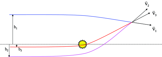
FIG. 1.: Schematic illustration of the effect of solar gravity on a CDM flow. Downstream of the Sun there are three flows, whereas upstream there is only one flow. The surface separating the two regions is the location of a caustic called the ’skirt’. It is a cone with opening angle equal to the maximum scattering angle of particles in the flow.

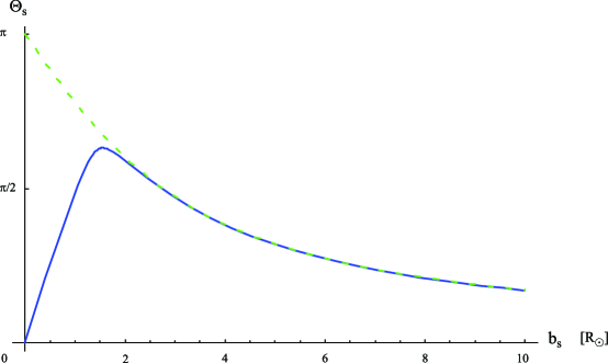
FIG. 2.: The scattering angle $\Theta_{\rm s}$ versus impact parameter $b_{\rm s}$, for the solar model of ref. [30] and incoming flow speed $v_{0}=265$ km/s. The dotted line is for a point mass Sun.

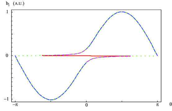
FIG. 3.: The impact parameters $b_{i}~{}(i=1,2,3)$ versus polar angle, defined relative to the incoming flow direction $\hat{v}_{0}$, at the Earth’s distance from the Sun, for the solar model of ref. [30] and incoming flow speed $v_{0}=265$ km/s. The dotted line is for a point mass Sun. When $|\theta|$ exceeds the maximum scattering angle, there is only one flow and hence only one value ($b_{1}$) of the impact parameter. When $|\theta|$ is less than the maximum scattering angle, there are three flows and three values ($b_{1},b_{2}$ and $b_{3}$) of the impact parameter.

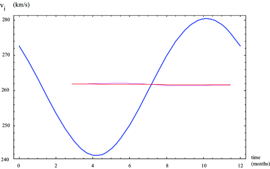
FIG. 4.: Flow speeds measured on Earth if the initial flow velocity is $\vec{v}^{5-}$, as a function of time of year, since Jan. 1. We neglect here the Earth’s rotation and the eccentricity of its orbit. Flows 2 and 3 exist on Earth from approximately March 30 until approximately Dec. 15. Their speed modulation is very small. Flow 1 exists throughout the year. Its speed modulation is of order 7%. The speed on Earth of flow 1 is largest near November 10 and lowest near May 10.

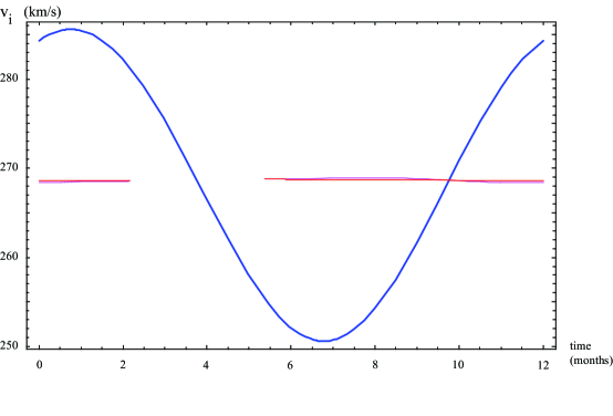
FIG. 5.: Same as Fig. 4 but with initial flow velocity equal to $\vec{v}^{5+}$. Flows 2 and 3 exist on Earth from approximately June 13 until approximately March 7. The speed of flow 1 is largest near Jan. 20 and lowest near July 20.

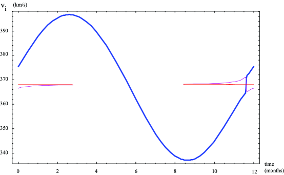
FIG. 6.: Same as Figs. 4 and 5 but with initial flow velocity equal to $\vec{v}^{10+}$, whose direction is close to the ecliptic. The Earth passes near the flow’s spike caustic on approximately Dec. 20.

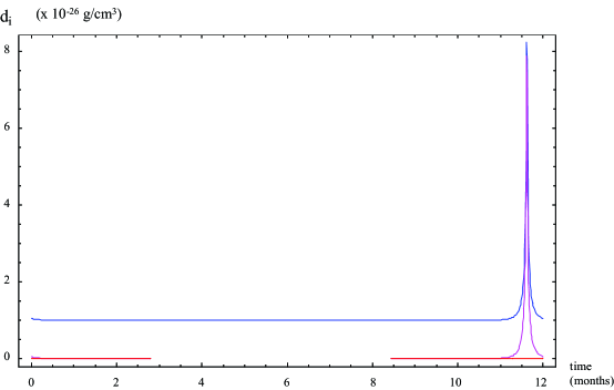
FIG. 7.: Flow densities $d_{i}~{}(i=1,2,3)$ on Earth for flow 10+, as a function of time of year. The flow speeds for this case are shown in Fig. 6. The Earth passes near the flow’s spike caustic on approximately Dec. 20. If $v_{Z}^{10+}=0$ the densities of flows 1 and 2 diverge at that moment. In Figs. 6 and 7, we used $v_{Z}^{10+}=2.6$ km/s, as an example. The Earth passes through the skirt caustic on approximately September 15 and March 25. However the associated divergences of the density of flows 2 and 3 are too feeble to show up on the graph.

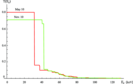
FIG. 8.: The function $T(E_{r})$, defined in Eq. (65), for the caustic ring model if the big flow has velocity $\vec{v}^{5-}$, at those times of year when the speed of the big flow relative to Earth is largest(May 10) and smallest (Nov. 10). For all $n$, the density $d_{n}^{\pm}$ was taken to be that of the flow with velocity $\vec{v}^{n\mp}$. To establish the scale on the horizontal axis, we set the WIMP mass $m_{\chi}=100$ GeV and target nucleus mass $m_{N}=Am_{\rm proton}$ with $A=73$. For different values of $m_{\chi}$ and $A$, rescale the horizontal axis by a factor proportional to $m_{r}^{2}/m_{N}$ where $m_{r}$ is the reduced mass.

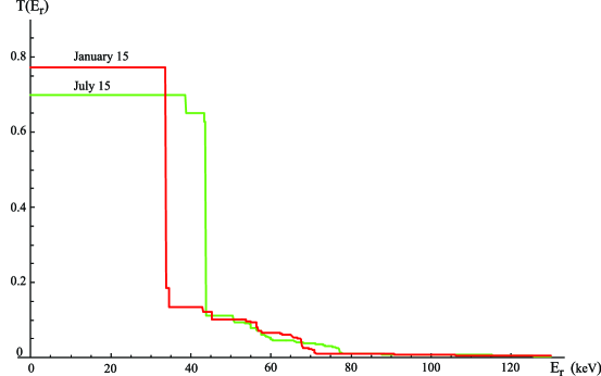
FIG. 9.: Same as Fig. 8 except that now the big flow has velocity $\vec{v}^{5+}$ and, for all $n$, $d_{n}^{\pm}$ is taken to be the density of the flow with velocity $\vec{v}^{n\pm}$.

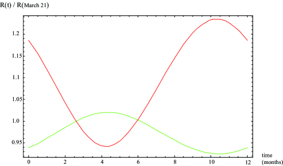
FIG. 10.: Event rate for the DAMA experiment in the 2-6 keV_ee range, as a function of time of year, for $m_{\chi}=50$ GeV (top curve) and $m_{\chi}=120$ GeV (bottom curve), relative to the event rate on March 21. The velocity of the big flow was taken to be $\vec{v}^{5-}$, as in Fig. 8. Spin-independent WIMP-nucleus couplings were assumed and the form factors were set equal to one.

REFERENCES

- [1] C.L. Bennett et al., Ap. J. Suppl. 148 (2003) 1.
- [2] S. Perlmutter et al., Ap. J. 517 (1999) 565; A. Riess et al., Astron. J. 116 (1998) 1009.
- [3] F. Zwicky, Helv. Phys. Act. 6 (1933) 110.
- [4] V.C. Rubin and W.K. Ford, Ap. J. 159 (1970) 379; D.H. Rogstad and G.S. Shostak, Ap. J. 176 (1972) 315.
- [5] P.J.E. Peebles, Ap. J. 263 (1982) L1; J. Ipser and P. Sikivie, Phys. Rev. Lett. 50 (1983) 925; G.R. Blumenthal, S.M. Faber, J.R. Primack and M.J. Rees, Nature 311 (1984) 517.
- [6] S. Tremaine and J.E. Gunn, Phys. Rev. Lett. 42 (1979) 407; J.R. Bond, G. Efstathiou and J. Silk, Phys. Rev. Lett. 45 (1980) 1980.
- [7] R.D. Peccei and H. Quinn, Phys. Rev. Lett. 38 (1977) 1440 and Phys. Rev. D16 (1977) 1791; S. Weinberg, Phys. Rev. Lett. 40 (1978) 223; F. Wilczek, Phys. Rev. Lett. 40 (1978) 279.
- [8] J. Preskill, M. Wise and F. Wilczek, Phys. Lett. 120B (1983) 127; L. Abbott and P. Sikivie, Phys. Lett. 120B (1983) 133; M. Dine and W. Fischler, Phys. Lett. 120B (1983) 137. For a discussion of the various contributions to the axion cosmological energy density, see S. Chang, C. Hagmann and P. Sikivie, Phys. Rev. D59 (1999) 023505.
- [9] H. Goldberg, Phys. Rev. Lett. 50 (1983) 1419; J. Ellis et al., Nucl. Phys. B238 (1984) 453.
- [10] P. Hut, Phys. Lett. 69B (1977) 179; B.W. Lee and S. Weinberg, Phys. Rev. Lett. 39 (1977) 183; M.I. Vysotskii, A.D. Dolgov and Y.B. Zel’dovich, JETP Lett. 26 (1977) 165; J.E. Gunn et al., Ap. J. 223 (1978) 1015.
- [11] P. Sikivie, Phys. Rev. Lett. 51 (1983) 1415, and Phys. Rev. D32 (1985) 2988; S. DePanfilis et al., Phys. Rev. Lett. 59 (1987) 839; C. Hagmann et al., Phys. Rev. D42 (1990) 1297; I. Ogawa, S. Matsuki and K. Yamamoto, Phys. Rev. D53 (1996) 1740; R. Bradley et al., Rev. Mod. Phys. 75 (2003) 777.
- [12] C. Hagmann et al., Phys. Rev. Lett. 80 (1998) 2043; S. Asztalos et al., Phys. Rev. D64 (2001) 092003; S. Asztalos et al., Ap. J. 571 (2002) L27.
- [13] M.W. Goodman and E. Witten, Phys. Rev. D31 (1985) 3059; I. Wasserman, Phys. Rev. D33 (1986) 2071; A. Drukier, K. Freese and D.N. Spergel, Phys. Rev. D33 (1986) 3495.
- [14] J.R. Primack, D. Seckel and B. Sadoulet, Ann. Rev. Nucl. Part. Sci. 38 (1988) 751; P.F. Smith and J.D. Lewin, Phys. Rep. 187 (1990) 203; G. Jungman, M. Kamionkowksi and K. Griest, Phys. Rep. 267 (1996) 195.
- [15] J.N. Bahcall and R.M. Soneira, Ap. J. Suppl. 44 (1980) 73; J.A.R. Caldwell and J.P. Ostriker, Ap. J. 251, (1981) 61; M.S. Turner, Phys. Rev. D33 (1986) 889; R.A. Flores, Phys. Lett. B215 (1988) 73.
- [16] A. Drukier, K. Freese and D. Spergel, Phys. Rev. D33 (1986) 3495; K. Freese, J. Frieman and A. Gould, Phys. Rev. D37 (1988) 3388.
- [17] D. Lynden-Bell, Mon. Not. R. Astron. Soc. 136 (1967) 101.
- [18] P. Sikivie and J.R. Ipser, Phys. Lett. B291 (1992) 288.
- [19] P. Sikivie, I. Tkachev and Y. Wang, Phys. Rev. Lett. 75 (1995) 2911, and Phys. Rev. D56 (1997) 1863.
- [20] J.A. Filmore and P. Goldreich, Ap. J. 281 (1984) 1; E. Bertschinger, Ap. J. Suppl. 58 (1985) 39.
- [21] P. Sikivie, Phys. Lett. B432 (1998) 139.
- [22] P. Sikivie, Phys. Rev. D60 (1999) 063501.
- [23] S. Tremaine, Mon. Not. R. Astron. Soc. 307 (1999) 877.
- [24] J.F. Navarro, C.S. Frenk and S.D.M. White, Ap. J. 462 (1996) 563; B. Moore et al., Ap. J. Lett. 499 (1998) L5.
- [25] F.S. Labini, T. Baertschiger and M. Joyce, astro-ph/0207029, to appear in Europhysics Letters; J. Diemand, B. Moore, J. Stadel and S. Kazantzidis, MNRAS 348 (2004) 977.
- [26] D. Stiff and L.M. Widrow, Phys. Rev. Lett. 90 (2003) 211301;
- [27] P. Sikivie, astro-ph/9810286, published in the Proceedings of the Second International Workshop on The Identification of Dark Matter, edited by N. Spooner and V. Kudryavtsev, World Scientific 1999, p.68, astro-ph/9810286.
- [28] P. Sikivie, Phys. Lett. B 567 (2003) 1; L. Duffy and P. Sikivie, in preparation.
- [29] W. Kinney and P. Sikivie, Phys. Rev. D61 (2000) 087305.
- [30] P. Sikivie and S. Wick, Phys. Rev. D66, 023504 (2002).
- [31] D. Stiff, L.M. Widrow and J. Frieman, Phys. Rev. D64 (2001) 083516.
- [32] K. Freese, P. Gondolo, H.J. Newberg and M. Lewis, astro-ph/0310334 and references therein.
- [33] J.D. Vergados, Phys. Rev. D63, (2001) 063511.
- [34] A.M. Green, Phys. Rev. D63 (2001) 103003.
- [35] G. Gelmini and P. Gondolo, Phys. Rev. D64 (2001) 023504.
- [36] R. Bernabei et al., Riv. N. Cim. 26 n.1 (2003) 1.
- [37] R. Abusaidi et al., Phys. Rev. Lett. 84 (2000) 5699.
- [38] A. Benoit et al., Phys. Lett. B513 (2001) 15.
- [39] J.C. Barton et al., in the Proceedings of the Fourth International Workshop on the Identification of Dark Matter, Sept. 2-6, 2002 in York, UK, edited by N.J.C. Spooner and V. Kudryavtsev, World Scientific 2003, p 302.
- [40] J. Binney and S. Tremaine, Galactic Dynamics, Princeton University Press, Princeton, NJ, 1987.
- [41] J. Binney and M. Merrifield, Galactic Astronomy, Princeton University Press, Princeton, NJ, 1998.