XMM Cluster Survey: X-ray source identification using the Sloan Digital Sky Survey

Abstract

The XMM Cluster Survey (XCS) is predicted to detect thousands of clusters observed serendipitously in XMM-Newton pointings. We investigate automating optical follow-up of XCS cluster candidates using the Sloan Digital Sky Survey (SDSS) public archive, concentrating on 42 XMM observations that overlap the First Data Release of the SDSS. Confining ourselves to the inner 11 arcminutes of the XMM field-of-view gives 637 unique X-ray sources across a $3.09\,{\rm deg^{2}}$ region with SDSS coverage. The log$N$–log$S$ relation indicates survey completeness to a flux limit of around $1\times 10^{-14}\,{\rm erg}\,{\rm s}^{-1}\,{\rm cm}^{-2}$ (in the 0.5-2.0 keV band).

We have used the SDSS data in a variety of ways. First, we have cross-correlated XMM point sources with SDSS quasars, finding 103 unique matches from which we determine a 90% confidence matching radius of 3.8 arcseconds. Using this matching radius we make immediate identifications of roughly half (214 of 520) of all XMM point sources as quasars (159) or stars (55). These objects will be a powerful resource for non-cluster studies. Second, we have estimated the typical error on SDSS-determined photometric cluster redshifts to be $\simeq 5\%$ for relaxed systems, and $\simeq 11\%$ for disturbed systems, by comparing photometric redshifts to spectroscopic redshifts for eight previously-known clusters ($0.183<z_{{\rm spec}}<0.782$). The measured level of error for disturbed systems may be problematic for X-ray and Sunyaev–Zel’dovich cluster surveys relying on photometric redshifts alone. Third, we use the False Discovery Rate methodology to select 41 XMM sources (25 point-like, 16 extended) statistically associated with SDSS galaxy overdensities. Of the 16 extended sources, 5 are new cluster candidates and 11 are previously-known clusters ($0.044<z<0.782$). There are 83 extended X-ray sources not associated with SDSS galaxy overdensities, which are our strongest candidates for new high-redshift clusters. We highlight two previously-known $z>1$ clusters that were rediscovered as extended sources by our wavelet-based detection software.

These results show that the SDSS can provide useful automated follow-up to X-ray cluster surveys, especially with regard to the rejection of point-source contamination, but cannot provide all the optical follow-up necessary for X-ray cluster surveys. Additional telescope resources must be employed to ensure their timely completion.

1 Introduction

The number density of galaxy clusters has the potential to provide important tests of the cosmological model (e.g. Evrard 1989; Henry & Arnaud 1991; Oukbir & Blanchard 1992; White, Efstathiou & Frenk 1993; Eke, Cole & Frenk 1996; Viana & Liddle 1996, 1999; Henry 1997; Eke et al. 1998). We describe here an ongoing effort to construct a new catalogue of clusters for cosmological studies, using X-ray data available in the XMM-Newton archive. This effort, known as the XMM Cluster Survey (XCS), has been described previously by Romer et al. (2001). By the end of the XMM mission, XCS is expected to include thousands of clusters of galaxies out to redshifts well beyond one. Optical follow-up of cluster candidates is one of the key challenges facing both X-ray and Sunyaev–Zel’dovich (e.g. Carlstrom, Holder & Reese 2002) surveys for distant clusters. In the past this was achieved using dedicated follow-up programmes that took many years to complete (e.g. Romer et al. 2000; Perlman et al. 2002; Mullis et al. 2003; Gioia et al. 2003). However, with the recent emergence of the “Virtual Observatory” (Szalay & Gray 2001) and datasets such as the Sloan Digital Sky Survey (SDSS; York et al. 2000), it should be possible to reduce the time spent on optical follow-up work. A first application of this to X-ray cluster surveys has been made by Schuecker, Böhringer & Voges (2004) using SDSS and ROSAT All Sky Survey (RASS) data.

This paper presents preliminary results from the matching of SDSS data with the XCS. In Section 2, we discuss the XMM data and outline our methods for analyzing it and determining the extent of X-ray sources. Section 3 describes the SDSS data we use for optical identifications; we use this to discuss positional accuracy of the source matching, associations with overdensities of optical galaxies, and photometric redshifting. In Section 4, we analyze the properties both of matched sources and of cluster candidates detected only in one of the wavebands. Throughout this paper, we assume a concordance flat cosmology ($\Omega_{{\rm m}}=0.3$, $\Omega_{\Lambda}=0.7$, $h=0.75$) with a cosmological constant. Fluxes are given in the ($0.5$–$2.0$) keV band unless otherwise stated.

2 X-ray Data Analysis

The XCS will process all EPIC imaging data available in the XMM archive. As of April 2003, 766 XMM pointings had been reduced using the XCS pipeline — see Figure 1. For this paper however, we restrict ourselves to 42 XMM pointings that lie within the SDSS first data release (DR1) spectroscopic area (Abazajian et al. 2003, henceforth A03). The SDSS DR1 comprises 2099 square degrees of five-band (u, g, r, i, z) imaging data, and 186,240 spectra of galaxies, quasars, stars selected over 1360 square degrees of the imaging area. In Table 1, we present the observation identification number (column 1) and coordinate (column 2) of each pointing, together with the designated target name and classification (column 3). Where available, we list in column 4 the target redshift according to the NED database. We list the number of sources detected (Section 2.2) within an off-axis distance $\theta<11$ arcminutes in column 5. For pointings with only partial SDSS coverage (indicated in column 8), we also give the number of $\theta<$11 arcminutes sources with SDSS overlap in parentheses; there are 50 sources detected in one or more of the pointings that do not overlap with the SDSS DR1. The maximum exposure time in seconds, after flare rejection (Section 2.1), is given in column 6. The number of square XMM image pixels ($5.1$ arcseconds on a side) used to calculate the area of the survey for the log$N$–log$S$ relation is given in column 7. Pointings with $\geq 52,000$ active pixels in Table 1 (18 of the 42 pointings) correspond to Full Frame Mode pointings with almost complete XMM/SDSS DR1 overlap and where no masking of the XMM field-of-view was necessary.

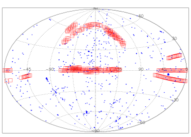
Figure 1: The 766 XMM pointings processed in the XCS project as of April 2003 are shown as blue points (equatorial projection). The SDSS-DR1 spectroscopic plates are indicated by red boxes. In each case, the symbol size indicates actual sky coverage.

Table 1: The 42 XMM Pointings with SDSS DR1 overlap. Certain pixels were not included when the survey area was calculated for the log$N$–log$S$ relation: 1) pixels surrounding an off-axis extended source, 2) pixels surrounding an extended target, 3) pixels not read out during small-window mode observations.

Obs. ID	J2000	Target (Type)	$z$	Sources	Time	Pixels	Notes
0002940401	03 41 16.2, -01 18 58.6	NGC1410 (AGN)	0.025	7 (2)	7094	20942	Partial SDSS overlap
0012440101	00 56 20.1, -01 19 30.6	LBQS0053-0134 (QSO)	2.063	16 (2)	28327	5175	Partial SDSS overlap, 1
0042341301	23 37 46.7, 00 15 35.1	RXCJ2337.6+0016 (Clus)	0.273	14	13132	45836	1, 2
0044740201	11 50 43.2, 01 44 17.7	Beta Vir (F Star)		32 (25)	47724	52218	Square hole in SDSS around target
0051760101	12 46 36.3, 02 20 25.1	PG 1244+026 (AGN)	0.048	9	12035	52222
0056020301	02 56 37.9, 00 04 59.7	RX J0256.5+0006 (Clus)	0.360	18	20664	52153
0060370101	15 43 56.5, 54 00 48.2	SBS 1542+541 (QSO)	2.371	12	8331	52171
0060370901	15 43 55.7, 54 00 43.4	SBS 1542+541 (QSO)	2.371	25	25098	52160
0065140101	00 41 48.1, -09 23 10.7	Abell 85 (Clus)	0.044	9	12380	37076	2
0065140201	00 42 36.8, -09 42 10.1	Abell 85 (Clus)	0.044	12	12379	52185
0066950301	23 18 10.2, 00 17 04.9	NGC 7589 (Galaxy)	0.0298	5	10833	52197	Missing stripe in SDSS
0066950401	23 18 21.5, 00 14 59.6	NGC 7589 (Galaxy)	0.0298	9	12360	52198
0081340801	12 13 44.8, 02 50 22.6	IRAS12112+03 (Galaxy)	0.072	22	22295	52210
0084230401	01 52 47.3, 00 59 42.1	Abell 267 (Clus)	0.230	22	17122	47177	2
0084230601	9 17 54.9, 51 41 57.1	Abell 773 (Clus)	0.217	11	14140	42722	2
0085640201	9 35 47.1, 61 22 44.0	UGC 05101 (AGN)	0.0394	36	33340	52154
0090070201	00 43 25.2, 00 50 16.1	UM 269 (QSO)	0.3084	24	20204	40104	1
0092800101	08 31 37.8, 52 46 52.8	APM 08279+5255 (QSO)	3.870	19	16520	52159
0092800201	08 31 46.5, 52 43 41.4	APM 08279+5255 (QSO)	3.870	47	72289	52132
0093030101	13 11 28.3, -01 18 49.6	Abell 1689 (Clus)	0.1832	34	36996	52213
0093060101	12 04 26.4, 01 55 59.1	MKW4 (Clus)	0.0200	13	14090	47187	2
0093200101	12 58 46.9, -01 43 15.3	Abell 1650 (Clus)	0.0845	24	37576	39138	2
0093630101	02 41 00.0, -08 14 10.4	NGC 1052 (AGN)	0.0049	20	15446	52154
0093641001	01 43 07.6, 13 37 32.3	NGC 660 (AGN)	0.0028	8	11040	52600
0094800201	11 40 33.8, 66 09 55.8	MS1137.5+6625 (Clus)	0.7820	27	35734	52140
0101640201	01 59 44.8, 00 24 46.8	Mrk 1014 (QSO)	0.1630	18	9732	40071	3
0102040501	14 29 08.6, 01 15 30.2	Mrk 1383 (AGN)	0.0865	3	3228	40094	3
0108460301	23 54 03.4, -10 23 1.20	Abell 2670 (Clus)	0.0762	16	17298	41311	1
0108670101	10 23 38.2, 04 13 00.0	ZwCl 1021.0+0426 (Clus)	0.291	43	53020	46257	1
0110990201	12 27 20.0, 01 27 42.1	HI1225+01 (Galaxy)	0.0043	11	28566	52218
0111190701	12 42 46.5, 02 42 53.8	NGC 4636 (Galaxy)	0.0031	35	58547	37225	1
0111200101	02 42 35.5, 00 00 04.3	NGC 1068 (Galaxy)	0.0038	29 (28)	36128	48336	Small hole in SDSS data, 1
0111200201	02 42 35.6, 00 00 05.4	NGC 1068 (Galaxy)	0.0038	33 (32)	32662	48334	Small hole in SDSS data, 1
0113040801	01 20 33.1, -10 56 06.5	C2001		9 (4)	8407	14447	Partial SDSS coverage
0113040901	01 18 41.1, -10 39 49.8	C2001		5	9794	52240	Proton flaring particularly bad
0126700201	12 29 04.3, 02 00 06.9	3C 273off-1.5min (QSO)	0.1583	8	25098	47223	2
0126700501	12 29 10.1, 02 02 44.2	3C 273off+1.5min (QSO)	0.1583	2	9511	48400	2
0129350201	03 36 42.2, 00 36 31.5	HR1099 (G star)		3 (1)	6374	47109	Large section missing in SDSS, 2
0134540101	03 36 51.9, 00 34 16.4	HR1099 (G star)		13 (10)	22869	47108	Large section missing in SDSS, 2
0134540401	03 36 41.9, 00 36 28.0	HR1099 (G star)		11 (6)	11546	35687	Large section missing in SDSS, 3
0134540601	03 36 42.2, 00 36 21.5	HR1099 (G star)		24 (17)	35100	45792	Section missing in SDSS data, 2
0137551001	12 29 05.8, 02 04 23.4	3C 273 (QSO)	0.1583	2	8963	35744	3

2.1 XMM data reduction and flare cleaning

The raw XMM photon data was obtained from the data archive at XMM-Newton Science Operations Centre and reduced with the February 2003 version of the XCS pipeline. This pipeline uses the XMM Science Analysis System (SASv5.4.1) and a single set of Current Calibration Files (CCF) for mission specific data processing. In the February 2003 version, only the data from the EMOS1 camera were used (subsequent versions generate merged images from the EMOS1, EMOS2 and EPN cameras). A data summary file is generated and, via the Observation Data Files (ODF) access layer, the completeness of each set is checked. The event linearization for each imaging mode is processed using SAS tools emproc and epproc for EMOS and EPN cameras respectively.

The resulting event lists were checked for temporal filtering to clean up the high-energy ($>$ 10 keV) flaring periods due to solar protons, see below. A detailed study of the XMM background can be found in Lumb et al. (2002) and Read & Ponman (2003). The flare cleaning method we used is similar to that suggested by Marty et al. (2003) and involves an iterative 3$\sigma$ clipping. An example of this method can be seen in Figure 2. For each event list, we filtered the sets with (PATTERN$<=$12). All sets were also filtered for energy range 10keV$\leq$PI$\leq$15keV and the light curves were generated with 100 sec binning (where PI is “pulse height invariant channel”). The mean and standard deviation were calculated in the counts per bin, and successive 3$\sigma$ cuts of the high-count periods were applied until the change in the mean was negligible. Good time intervals were generated using the last mean and the standard deviation with a last 3$\sigma$ cut and used in filtering of the previously-prepared raw set with the aforementioned pattern selection and (FLAG == 0). Although this method of cleaning does not give a perfect filtering for all sets, it can be automated to clean thousands of pointings at once, as required for the XCS. Considering the varying quiescent mean in the high-energy background (Pratt & Arnaud 2002; Lumb et al. 2004), it is superior to defining a fixed cut for filtering.

After flare cleaning, the products used for source detection were generated: Detector masks, images and exposure maps in two energy bands ([0.5–2.0] and [2.0–10.0] keV) with $5.1$ arcsecond square pixels binning. Exposure maps include spatial quantum efficiency, filter transmission, mirror vignetting, and field-of-view information. The image products were then passed into the source detection algorithm.

Figure 2: This figure shows an example of the high-energy filtering method we used for each pointing. The data are from observation 0060370901. The lightcurves are generated for events with energies $>$ 10 keV with 100 sec binning. (a) The initial light curve is in blue/solid, and the mean of the uncut light curve is in red/dashed. (b) The same with reduced vertical scale. The decrease in the mean of the light curve using successive 3$\sigma$ cut cleaning can be seen from the mean of the remaining exposure which is in red/dashed. (c) The original high-energy light curve, now with the filtered flaring regions shown as red/dashed and the remainder as blue/solid.

2.2 Source detection

We identify sources detected in XCS fields using a wavelet-based algorithm. The key advantage of wavelets is the natural separation achieved between small- and large-scale variations in the data, e.g. a large-scale slowly-varying background will be filtered out of the small-scale signal, and therefore will not influence the detection of such sources [see also Vikhlinin et al. (1998), Romer et al. (2000) and Freeman et al. (2002)].

For the work presented herein, the source detection proceeded as follows. First, we performed a wavelet transform of the 2D XMM image using the à trous algorithm (e.g. Holschneider et al. 1989; Shensa 1992) to produce, for each spatial scale, a 2D image of wavelet coefficients from which we must remove noise, i.e. determine which coefficients are statistically significant. One complication here is the small-number statistics for the photons in the X-ray background of our images. To accommodate this problem, we have adopted the “wavelet histograms” approach of Starck & Pierre (1998) as implemented in their MR/1 software package, in particular the task mr_detect. Briefly, the software first identifies all pixels in a wavelet coefficient image that are above a confidence level, specified by the user, after modelling the low count rate Poisson noise in the images. These significant pixels in each wavelet plane are connected to form the “segmentation image” at that scale. A set of connected wavelet coefficients is known as a structure and structures within different wavelet planes are connected to form objects by way of the interscale relation. A structure $S_{j}^{1}$ at scale $j$ is said to be connected to a structure $S_{j+1}^{2}$ at scale $j+1$ if $S_{j+1}^{2}$ contains the pixel in $S_{j}^{1}$ with the maximum wavelet coefficient. In this way objects can be identified in wavelet-transform space and can be divided into sub-units of the main source (i.e. de-blended). The objects are then reconstructed iteratively using a 2D Gaussian and the counts associated with each object computed. The local exposure time gives the rate in counts per second. We then use energy conversion factors to obtain the flux, depending on the absorption factor $n_{{\rm H}}$ and the type of filter used. The fluxes of our sources were calculated with energy conversion factors (ECFs) generated as recommended by Osborne (2003), using the canned response matrices released on 2003-01-29 and ancillary response files generated for each filter type on the optical axis for the pattern selection specified in Section 2.1. To take the effect of the column density of neutral hydrogen in the direction of each XMM pointing into account, we generated tables of ECFs for a subset of possible $n_{{\rm H}}$ values. The $n_{{\rm H}}$ values of the pointings were obtained using one of the FTOOLS, nH, which uses the HI map by Dickey & Lockman (1990) as a basis.

Figure 3: The log$N$–log$S$ relation (black dots) for XCS sources in a $3.09\,{\rm deg^{2}}$ region overlapping the SDSS DR1 area. The hatched region is the observed range taken from Baldi et al. (2002). The dot-dashed lines are error bounds for the XMM log$N$–log$S$ in the HDF–North region (Miyaji et al. 2003).

When no cut in off-axis distance is applied, we detect 1121 X-ray sources within the 42 XMM pointings presented in Table 1. This number includes duplicate detections (in overlapping pointings), the primary (usually on-axis) target of the respective pointing, and regions without SDSS DR1 coverage. We define a duplicate detection to be one that falls with 5 arcseconds of a source detected in a different pointing. Throughout this paper, we concentrate on those 740 sources that lie within $\theta=11$ arcminutes of the pointing center, i.e. where the XMM PSF is well-behaved.

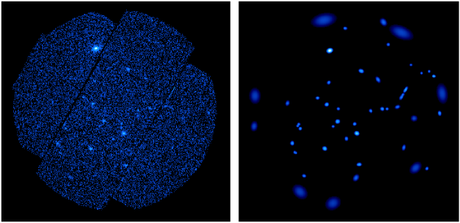
Figure 4: On the left we present a sample XMM image, and on the right we show the location and size of sources detected by the à trous algorithm.

In Figure 3 we present the $\theta<11$ arcminutes log$N$–log$S$ relation for the 42 pointings in Table 1. To create this figure, we have removed duplicate detections, primary targets and sources in regions without SDSS DR1 overlap. We determined that there is a unique overlap area of $3.09\,{\rm deg^{2}}$ between the 42 pointings and the SDSS DR1. This area has been corrected for pointing overlaps, partial SDSS cover and any $\theta<11$ arcminutes regions masked (e.g. due to the presence of an extended target) or missing (e.g. because the observation was carried out in small-window mode) from the XMM field-of-view. We did not correct for the different sensitivities of the individual pointings when constructing the log$N$–log$S$ relation, but note that the exposure times are similar for most pointings and so this should not be a significant problem. Our log$N$–log$S$ relation is in excellent agreement with the published XMM log$N$–log$S$ relation of Baldi et al. (2002) to at least a flux limit of $1\times 10^{-14}\,{\rm erg}\,{\rm s}^{-1}\,{\rm cm}^{-2}$, which indicates that our parent catalogue is complete to this flux limit. Figure 3 demonstrates the quality of the XMM image processing pipeline. We do not make a fit to the log$N$–log$S$ relation, or attempt to model the incompleteness at fainter flux limits, as we are primarily interested in finding X-ray clusters of galaxies.

2.3 Extent classification

The next step is to classify the detected sources as extended or point-like. The XCS will use X-ray extent as the primary means by which to select cluster candidates; assuming no size evolution for clusters with redshift, we expect clusters to be resolved by XMM at any redshift (Romer et al. 2001). The challenges here are two-fold. First, the point-spread function (PSF) of XMM varies across the satellite field-of-view; this can be seen in Figure 4. Secondly, over 80% of all X-ray sources are point sources (AGNs, quasars, stars etc.), and therefore any misclassification of X-ray point sources as extended sources will swamp the underlying cluster population leading to laborious optical follow-up. Therefore, any extended source detection algorithm must address these two issues, as well as being sensitive to true extended sources. The completeness of any extended source catalogue will need to be determined via extensive simulations, as in Adami et al. (2000) and Burke et al. (2003).

For the work presented herein, we used a preliminary extended source detection algorithm based on the ratios of the wavelet coefficients for each source as calculated at the different wavelet scales. For example, the wavelet coefficients of point-source objects should be relatively higher at the smallest wavelet scales, and smaller at the larger scales; the reverse would be true for an extended source. We use the square of the modulus of the coefficients to provide a measure of the wavelet power at that scale and use the ratios of different scales to classify the sources. For our data, we have four wavelet scales (plus one low-resolution residual scale which is not used) and therefore we can calculate six wavelet ratios (not all independent) as

$$\hskip 85.35826ptR_{ij}=\frac{C_{i}^{2}}{C_{j}^{2}},\quad i<j\,,$$

where $C_{i}$ denotes the wavelet coefficient at the pixel closest to the source position at one of the four wavelet scales available to us.

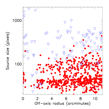
Figure 5: The number of pixels enclosed by the XCS source ellipses versus off-axis distance. The solid circles show point-like sources (score $\leq 1$), while the open triangles are extended sources (score $\geq 3$). We note that the large on-axis sources are known, targeted, nearby clusters of galaxies (see Section 4.2).

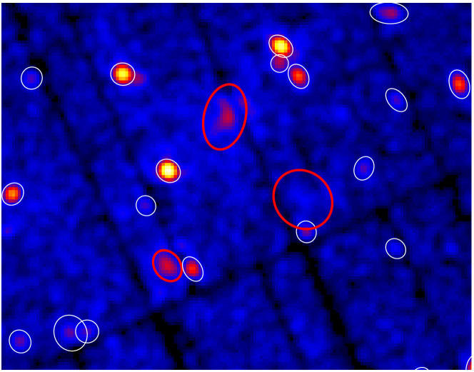
Figure 6: Part of a (smoothed) XMM image showing three high-redshift clusters redetected by XCS (thick rings); RDCS J0849+4452 ($z=1.265$; lower left), RX J0848.7+4457 ($z=0.574$, SHARC cluster, top) and RDCS J0848+4453 ($z=1.273$, lower right) (Hashimoto et al. 2002). The size of the ellipses reflects the detected size of each object, showing that these high-redshift clusters are resolved in this XMM data. The clusters are classified as extended using our wavelet-ratio test, while the remaining objects in the image are all classified as point-like. For illustrative purposes we have shown the EPN image data, but the source detection/parametrization was carried out in EMOS1, consistent with the other work presented herein.

For each of the XMM/SDSS fields we used a combination of NED associations and eyeballing to classify the sources found as either point-like, extended, unknown or artifacts. When the various combinations of ratios were plotted against each other it was found that there was differentiation between these classifications, such that empirical cuts could be made to separate extended and point-like sources. We use these ratios as a crude extent classification, and extended sources can be efficiently separated from point-like sources using the following selection criteria:

$R_{14}<12.5\,\times R_{12}$  or  $R_{14}<4\,\times R_{13}$,

$R_{23}<2$,

$R_{24}<11$,

$R_{34}<5$.

For each of these four criteria, we award each source a score of one, so sources can have scores ranging from zero to four on this scale. To confirm that these cuts were reasonable we calculated the histogram of extent scores found using them. The distribution for sources classified as point-like showed that 90% had extent scores of 0 or 1, and similarly 90% of the extended sources had scores of 3 or 4. For the remainder of this paper, we use these scores as our classification of whether a source is extended or not. In Figure 5 we present the size (as the number of pixels enclosed by the source ellipse) of all detected sources as a function of off-axis distance. This demonstrates that there are two distinct populations of sources, regardless of off-axis distance, and that our extent classification can successfully separate them.

To demonstrate the effectiveness of the method, we show in Figure 6 a 39 ksec XMM pointing (not in the SDSS DR1 area) toward three previously-known high-redshift clusters, all three of which were classified as extended by our algorithm. Of the 740 ($\theta<11$ arcminute) sources mentioned in Section 2.2, 112 ($\simeq 15\%$) have extent scores $\geq 3$. These 112 include duplicate detections and sources falling in regions of the XMM field-of-view not covered by SDSS DR1. We discuss the 99 unique extended sources with SDSS DR1 coverage in Section 4.

We have tested the robustness of our extent algorithm using 59 duplicate detections. These sources lie in regions that overlap between different XMM pointings. We found that the source classifications agreed in 53 cases (90%). For the 6 sources that disagreed, 5 of them are extremely bright point sources, with count rates exceeding $1$ count per second. In these cases, the detailed structure of the PSF is detected and the source appears extended rather than a point source. If we exclude very bright sources, the classifications agreed $98\%$ of the time.

We note that, subsequent to the work presented herein, we have developed more sophisticated detection and classification algorithms. We now use a modified version of WAVDETECT (Freeman et al. 2002), rather than MR/1, to perform the wavelet transforms. WAVDETECT has the advantage that we can use exposure map information, something that is vital for the analysis of merged (EMOS1+EMOS2+EPN) images. Furthermore, the extent classification now uses models of the PSF provided in the CCFs [see Davidson et al. (in preparation) for more details].

3 Optical Identifications using SDSS

We have extracted from the SDSS DR1 website all data available within a radius of 25 arcminutes around each of the 42 XMM pointing centers listed in Table 1. Eleven of the 42 have only partial SDSS coverage, as described in the table comments. As X-ray point sources (e.g. stars and quasars) tend also to be optical point sources, we have made use of the SDSS PHOTO flag objtype for this study. This flag classifies optical sources as either point-like (objtype=6, e.g. star, quasar), or extended (objtype=3, e.g. galaxy) and works well to ${\rm r}=20.5$. At fainter magnitudes we have assumed everything is a galaxy (since galaxies dominate the faint-end number counts). When SDSS spectra are available, we can extract object redshifts and/or spectroscopic classifications (spec_class). Even when spectra are not available, we can still make use of the results from the SDSS spectroscopic target algorithms. These algorithms were designed to select particular types of sources from the SDSS multi-color photometry for spectroscopic follow-up. Many more targets are selected than can be allocated optical fibres, e.g. there are 16998 official SDSS quasar targets in our study region alone.

In addition to the official SDSS target information, we use an extra quasar classification flag (QSOcol) based on the colour–colour diagrams of Richards et al. (2001; see Figure 4 in their paper). From these diagrams, it is clear that quasars predominately inhabit a volume of colour–colour space as defined by: $-0.2<{\rm u}-{\rm g}<0.7$, $-0.2<{\rm g}-{\rm r}<0.6$, $-0.2<{\rm r}-{\rm i}<0.6$, and $-0.2<{\rm i}-{\rm z}<0.5$. Therefore, if an SDSS object satisfies these colour cuts, we flag it as QSOcol$=1$. Overall, 7443 objects were flagged in this way, of which only 1550 were already amongst the 16998 official SDSS quasar targets. We use these QSOcol$=$1 objects in Sections 3.1 & 4.1.

Figure 7: The absolute scatter seen in the RA and DEC, as a function of off–axis distance, for the 182 matches between SDSS quasar candidates and XMM sources.

3.1 Positional accuracy

We have used the SDSS to derive the matching radius appropriate for the optical follow-up of XCS sources. It is important that this radius be as small as possible to cut down on erroneous matches. To do this, we have made use of the fact that optical quasars should have a point-like X-ray counterpart. We have compared XCS point sources (i.e. those with an extent score of $\leq 1$) that match, within an initial search radius of 10 arcseconds, to a single SDSS point-like object (i.e. objtype$=$6). Further, this single SDSS object must have been spectroscopically classified by the SDSS as a quasar, or be one of the 16998 official quasar candidate targets.

We find a total of 182 matches (no off-axis distance limit). These matches give an RMS of $3.8$ arcseconds for the total separation between the X-ray and optical centroid. We also find an RMS of $\delta_{{\rm RA}}=2.8$ arcseconds for the difference in Right Ascension and an RMS of $\delta_{{\rm DEC}}=2.6$ arcseconds for the difference in Declination for these matches. We show the scatter of $\delta_{{\rm RA}}$ and $\delta_{{\rm DEC}}$ with off-axis distance for these 182 matches in Figure 7, and the rms values in Table 2. We see an increase in the scatter toward higher off-axis distances, which is to be expected due to the increase in size of the XMM point-spread function with off-axis distance. In the following, we therefore limit ourselves to the 103 matches at off-axis distances less than $\theta=11$ arcminutes.

Table 2: The error in arcseconds in matching sources as a function of off-axis distance.

Off-axis	Matches	rms $R$	rms $\delta_{{\rm RA}}$	rms $\delta_{{\rm DEC}}$
All	182	3.8	2.8	2.6
$\theta<$8 arcmin	73	3.4	2.6	2.3
$\theta<$11 arcmin	125	3.7	2.9	2.4
$\theta>$11 arcmin	57	4.0	2.8	2.9

Figure 8: The histogram of separations for the 103 SDSS quasars with XCS counterparts.

In Figure 8, we present the distribution of absolute separations between the optical and X-ray coordinates for 103 SDSS quasars. If the errors in the RA and DEC are Gaussian distributions of equal variance about zero, and the background sources negligible, the separations should follow a $\chi^{2}_{2}$ distribution, whose variance equals its mean. However, those assumptions do not appear to be valid, so we instead fit individual Gaussians to the observed $\delta_{{\rm RA}}$ and $\delta_{{\rm DEC}}$ distributions for our 103 quasar candidates. We find means of -0.4 and -0.6 arcseconds respectively, with dispersions of 1.9 and 1.4 arcseconds. The distribution of separations is slightly elongated in the RA direction, as can be seen in Figure 9. The non-zero mean values indicate that there is a systematic pointing offset, i.e. errors in the boresight of each pointing, thus introducing a systematic error in the coordinates of all sources in that pointing.

Figure 9: The scatter in $\delta_{{\rm RA}}$ and $\delta_{{\rm DEC}}$ for 103 SDSS quasars with XCS counterparts, with the dashed ring indicating the rms offset.

Furthermore, we note that the background sources are beginning to dominate the source counts as we approach 10 arcsecond separation. Therefore, we refined our analysis by including a linear function in our fit to the distribution of separations to account for the background contamination, i.e. we fit a Gaussian plus a linear function. The best-fit for the Gaussian part now has a mean of 1.8 arcseconds and dispersion of 1.2 arcseconds. Note that it is the mean which estimates the typical positional error, while the dispersion carries information about the width of the distribution. We assume that matches within the 90% confidence range of the Gaussian part are likely to be true matches, obtaining a matching radius of $1.8+1.65\times 1.2=3.8$ arcseconds.

As a check of our determination of the matching radius, we split the sample of 103 quasar candidates into bright and faint subsamples, with a dividing flux of $1.2\times 10^{14}\,{\rm erg}\,{\rm s}^{-1}\,{\rm cm}^{-1}$. We found that each subsample gave the same 90% matching radius of 3.8 arcseconds using the prescription above. We also checked duplicate (Section 2.3) X-ray sources and found the mean separation between these sources to be consistent with this matching radius. Furthermore, if we include a further 123 QSOcol sources (see above for definition) in our analysis, our matching radius does not change. The size of the XCS matching radius will be dominated by the positional errors in the X-ray data, as the absolute astrometric calibration of the SDSS is accurate to less than 0.1 arcseconds (Pier et al. 2003) for point sources. Our matching radius of $3.8$ arcseconds is similar to the 5 arcseconds suggested by Watson et al. (2002), but is somewhat larger than that found by Altieri (2002). Altieri used matches with the USNO catalogue to estimate individual XMM pointing offsets. He found a systematic pointing offset of $\simeq 0.3$ arcseconds, with a mean offset of one arcsecond. Therefore, our $3.8$ arcseconds matching radius likely includes two contributions, an error from the centroiding of the sources and a systematic pointing offset.

3.2 Optical overdensity

While the XCS is a serendipitous X-ray survey, with clusters to be discovered initially in XMM data, many such clusters will also be detectable in the optical as an overdensity in the projected galaxy distribution. We have therefore calculated the overdensity of SDSS galaxies around each of the X-ray sources in our study region, by counting the number of galaxies within an aperture of radius 40 arcseconds centered on the centroid of the X-ray emission. This angular aperture was chosen to approximately equal the angular size of distant clusters that could be seen in the SDSS data; the typical core radius of a $z=0.35$ cluster (200kpc) subtends an angle of 41 arcseconds on the sky. The area enclosed by this radius ($\simeq 200$ pixels) is also in good agreement with the size of extended XCS sources (Figure 5).

We make a local background correction using the observed galaxy count within an annulus centered on the X-ray source with an inner radius of 80 arcseconds and the outer radius equal to 100 arcseconds (scaled by the area). This annulus corresponds to a radius of approximately half the virial radius for a $z=0.35$ cluster, and thus provides a local estimate of the projected galaxy density around each source. This annulus will be contaminated by cluster members, but this effect will be small.

For each source, we calculate two galaxy overdensities, once imposing a magnitude limit of ${\rm r}=22.2$ and once without a magnitude limit. The former is the completeness limit of the SDSS photometric survey (see A03), while the latter allows us to use the full dynamic range of the SDSS photometry. For example, by not imposing a magnitude limit we are effectively counting the number of galaxies detected in any of the 5 SDSS passbands, as PHOTO (the SDSS photometric analysis pipeline; Lupton et al. 2001) detects sources in all 5 passbands separately and reports upper limits, if necessary, in the other passbands if they are not detected. We stress again that for sources brighter than ${\rm r}=20.5$ we use the SDSS PHOTO objtype flag to identify galaxies, while below this limit, we simply call all objects galaxies. We also use any object spectroscopically confirmed to be a galaxy or listed as an official galaxy target. By using a local background correction, we guard against fluctuations both in the completeness of the SDSS photometric survey and in the star–galaxy separation at faint magnitudes.

To determine the statistical significance of any observed overdensity of galaxies around these X-ray sources, we construct the distribution of counts one would expect from random. This was achieved by placing the 40 arcsecond radius aperture on 10,000 randomly selected SDSS sources and making the same local background correction. We only consider SDSS sources from the XMM regions that have full SDSS coverage (see Table 1) and restrict our analysis to SDSS sources between 3 and 11 arcminutes from the centre of those pointings. We note that there are more than 10,000 SDSS sources that satisfy this criteria (mostly distant galaxies and faint stars) and their angular clustering is weak, less than 1% angular fluctuations within a 40 arcsecond aperture (Connolly et al. 2002), especially for the no-magnitude count distribution. We show the two count distributions in Figure 10. As expected the distribution for the no magnitude limit case distribution is broader. The distributions are well fit by a Gaussian with a mean and dispersion of $-0.11$ and 3.39 respectively for the no magnitude limit case and $-0.074$ and 2.86 for the $r=22.2$ limited case. We re-fit the Gaussian using only the count data between -5 and 5, but found consistent means and sigmas. We tried other methods for constructing the count distributions, e.g. randomly placing the apertures within the SDSS area, and found the results to be consistent.

Figure 10: The distribution of background corrected galaxy counts from both the no magnitude limit case (solid line) and the $r=22.2$ limited case (dashed line).

We have used the distributions presented in Figure 10 to define a threshold above which an observed SDSS overdensity is considered to be statistically significant. By design, such overdensities are ideal candidates for clusters of galaxies. To define this threshold, we have used the False Discovery Rate (FDR) statistical methodology as outlined in detail by Miller et al. (2001) and Hopkins et al. (2003). It has been applied to SDSS cluster selection in Miller et al. (2004). Briefly, FDR controls the ratio of the number of false detections over the total number of detections, and therefore is a more scientifically-meaningful quantity than selecting a fixed threshold based on a multiple of sigma, e.g. using a 3-sigma threshold. FDR is adaptive in that it changes based on the number of tests performed, while a standard sigma-based threshold is not adaptive and thus leads to many more false detections as the number of tests grows large. In summary, FDR is ideal for our problem, especially as it naturally accommodates correlated data which is the case here (see Miller et al. 2001).

The key parameter of FDR is $\alpha$, the ratio of false to true detections one is willing to tolerate. Here, we have selected $\alpha$ to be 0.25, i.e. we will allow up to 25% of our selected overdensities to be potentially false. Computationally, FDR is simple to implement and involves determining the probability that the observed SDSS count around each of our X-ray sources is drawn from the count distributions in Figure 10. These probabilities are then ranked and a threshold calculated using the methodology given in Miller et al. (2001). This was performed separately for both distributions featured in Figure 10. Using $\alpha=0.25$ we selected 39 candidate overdensities from each distributions, i.e. in both cases 39 of the 690 X-ray sources were assessed to lie in statistically-significant galaxy overdensities. There is significant overlap between the two lists, with 30 candidates in common giving 48 candidates in total. We discuss these 48 galaxy overdensities further in Section 4. For reference, the calculated FDR thresholds corresponds to a threshold of 2.20 sigma (an overdensity above 7.3) for the no magnitude limit distribution and 2.24 sigma (above 6.3) for the ${\rm r}<22.2$ count distribution.

3.3 Photometric redshifts

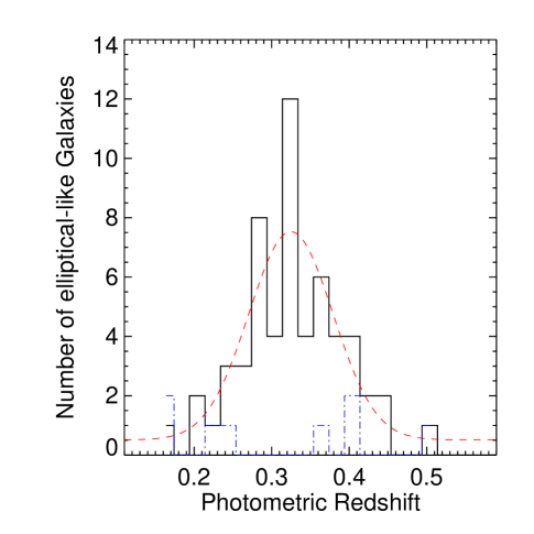
Figure 11: The photometric redshift histogram of cluster RXJ0256 (black line). The blue/dashed histogram represents the photometric redshift histogram for a randomly chosen location 1.3 degrees west of the cluster centroid. This demonstrates the significance of the peak seen in the black cluster histogram, which contains 60 sources compared to only 8 sources in the blue/dashed histogram.

Table 3: The classification of our 637 XMM sources.

Class	Number	Comments
0100	203	Not extended, one point-like SDSS match
0101	11	Not extended, two SDSS matches (at least one is point-like)
0000	296	Not extended, no point-like SDSS match (could have an SDSS galaxy match within $3.8^{\prime\prime}$)
0001	3	Not extended, two SDSS matches (neither are point-like)
1000	70	Extended, no point-like SDSS match (could have an SDSS galaxy match within $3.8^{\prime\prime}$ )
1101	2	Extended, two SDSS matches (at least one is point-like)
1100	11	Extended, one point-like SDSS match
1010	16	Extended, no point-like SDSS match, galaxy overdensity
0010	15	Not extended, no point-like SDSS match, galaxy overdensity (could have an SDSS galaxy match within $3.8^{\prime\prime}$)
0110	8	Not extended, one point-like SDSS match, and galaxy overdensity
0011	2	Not extended, two SDSS matches (neither are point-like), galaxy overdensity
0111	0	Not extended, two SDSS matches (at least one is point-like), galaxy overdensity
1111	0	Extended, two SDSS matches (at least one is point-like), galaxy overdensity
1110	0	Extended, one SDSS point-like match, galaxy overdensity
1011	0	Extended, two SDSS matches (neither are point-like), galaxy overdensity
1001	0	Extended, two SDSS matches (neither are point-like)

When SDSS data are available for a particular XCS cluster candidate, it may be possible to determine the cluster redshift without the need for additional dedicated spectroscopic follow-up. We have investigated how well we can recover the spectroscopic redshift for the $z>0.1$ clusters using photometric redshifts. Photometric redshift estimates are available for all galaxies in the SDSS DR1 (see Csabai et al. 2003; Budavári et al. 2003). Briefly, the SDSS DR1 database contains an estimate of both the redshift and spectral type ($t$), with errors, for each galaxy. For each $z_{{\rm spec}}>0.1$ cluster identified, we extracted these data from the DR1 in an aperture of radius 40 arcseconds (i.e. the same as was used for the optical overdensity measurements) centered on the X-ray centroid. We then excluded any galaxies with $z_{\rm photo}<0.05$, with a photometric redshift error of greater than the measured photometric redshift, or with a photometric spectral classification of $t\geq 0$. This last criterion ensures we are only considering “elliptical-like” galaxies which are likely to be cluster members (see Budavári et al. 2003 for a discussion of the $t$ parameter). We then fit the distribution of these remaining photometric redshifts with a Gaussian plus a constant (e.g. Figure 11) to accommodate outliers in redshift (mostly at redshifts greater than the cluster).

Alternative approaches would be to use the E/S0 ridgeline (e.g. Gal et al. 2000; Gladders & Yee 2000) or a matched filter technique. The latter technique has recently been applied to SDSS data by Schuecker et al. (2004). Based on 60 clusters detected using a joint RASS/SDSS search, they found an average redshift offset of $\sigma_{z}=0.03$, or 20% at their typical survey redshift ($z\simeq 0.15$).

4 Matched sources and cluster candidates

We now return to X-ray source identifications using SDSS data. We concentrate on XCS sources detected in one or more of the 42 pointings listed in Table 1 at off-axis distances of $\theta<11$ arcminutes. We detected 740 such sources, 690 of which also overlap with the SDSS DR1. Of these, 53 are duplicate detections, leaving 637 unique sources. Amongst these 637, 520 are point-like (extent score $\leq 1$) and 99 are extended (extent score $\geq 3$). The remaining 18 have an ambiguous classification (extent score $=2$); henceforth we will include them under the description ‘point-like’.

4.1 Source classification

In Table 3 we present the results of matching the 637 XMM sources with the SDSS DR1 data, using a matching radius of 3.8 arcseconds (Section 3.1) centered on the X-ray centroid. We also present the results of our search for galaxy densities (Section 3.2). To understand the SDSS–XMM match-ups, we use the following four binary criteria (0$=$no, 1$=$yes) when classifying all the XMM sources:

• Is the X-ray source extended (extent $\geq 3$)?

• Is there at least one SDSS point source (objtype$=6$) present within the 3.8 matching radius?

• Is there a significant overdensity of SDSS galaxies?

• Are there two SDSS sources within the 3.8 arcsecond matching radius? For this test, we include all SDSS objects i.e. also galaxies (objtype$=3$).

Each source has a 4-bit identification, e.g. 0011, 1010 etc., providing sixteen possible combinations. The ordering of the bits is as given in the list above. The breakdown of classifications for all 637 unique XMM sources in given in Table 3.

We find 214 point-like X-ray sources that match at least one point-like SDSS source ($0100+0101$): 55 of these SDSS point-like matches are stars, 159 are quasars. Therefore, we have been able to provide immediate identifications for 34% of all sources and can eliminate them from a cluster candidate list without any need for dedicated optical follow-up. We provide no further discussion herein of these 214 sources, beyond noting that such merged XMM/SDSS point-source catalogues will be a powerful resource for AGN/quasar science.

We find 299 (47% of the total) point-like X-ray sources that have no point-like SDSS counterpart ($0000+0001$). For these, we cannot make an immediate classification based on SDSS data alone. Most of them will be optically-faint stars or active galaxies/quasars and are not of an immediate relevance to the XCS science goals. However, we note the three $0001$ cases, where an X-ray point source lies within $3.8$ arcseconds of two SDSS galaxies. For these, we may be seeing a few brightest cluster galaxies and further optical follow-up is merited. By contrast, we do not plan to pursue dedicated optical follow-up of the 296 objects with the $0000$ flag. A small fraction of them may be clusters or groups. However, they have neither been flagged as galaxy overdensities in the SDSS or as extended by our X-ray pipeline. The XCS extent algorithm works even at high redshifts (see Figure 6), but only given a high enough signal-to-noise. To simplify the XCS selection function, we are adopting a conservative signal-to-noise threshold (see Romer et al. 2001). Any clusters in the $0000$ category must be low signal-to-noise detections and would not be suitable for inclusion in the XCS cluster catalogue.

Table 4: Known clusters in our XMM pointings. Those above the line were target clusters, listed in Table 1. The fluxes are in units of $10^{-12}$ erg s^-1 cm^-2. We estimated photometric redshifts only for clusters with $z_{{\rm spec}}>0.1$.

Cluster	Extent	Major axis	Minor axis	Off-axis angle	Counts	Flux	SDSS	$z_{{\rm photo}}$	$z_{{\rm spec}}$
	Score	(arcmin)	(arcmin)	(arcmin)	(s-1)		overdensity
RXCJ2337.6+0016/Abell 2631	4	2.42	1.71	0.81	0.212	1.094	yes	$0.26\pm 0.02$	0.273
RX J0256.5+0006	4	1.13	0.85	0.26	0.035	0.193	yes	$0.32\pm 0.05$	0.36
RX J0256.5+0006 (subclump)	4	0.75	0.58	0.68	0.008	0.043	yes	$0.32\pm 0.05$	0.36
Abell 85	4	1.15	1.12	6.19	0.022	0.111	yes		0.044
Abell 267	4	1.95	1.51	0.16	0.242	1.243		$0.23\pm 0.03$	0.23
Abell 773	4	2.06	1.73	0.14	0.298	1.457	yes	$0.21\pm 0.02$	0.217
Abell 1689	4	1.69	1.58	0.05	1.00	4.909		$0.19\pm 0.04$	0.1832
MKW4	4	0.85	0.78	0.58	0.251	1.257	yes		0.02
Abell 1650	4	2.31	1.67	1.72	0.853	4.281			0.0845
MS1137.5+6625	4	1.06	0.99	0.44	0.022	0.107	yes		0.7820
Abell 2670	4	0.91	0.81	1.62	0.038	0.196			0.0762
Abell 2670 (subclump)	4	0.38	0.33	1.34	0.013	0.065			0.0762
ZwCl 1021.0+0426	4	0.88	0.74	0.23	0.489	2.461	yes	$0.27\pm 0.03$	0.291
VMF98-116	4	1.75	1.18	5.82	0.017	0.083	yes	$0.36\pm 0.02$	0.409
VMF98-021	4	0.79	0.60	10.55	0.034	0.176	yes	$0.35\pm 0.03$	0.386
SDSS CE J010.717058	4	1.15	0.97	10.65	0.004	0.018	yes

More interesting to the XCS are the 70 extended X-ray sources (category 1000) that have no SDSS counterpart (point-like or galaxy). Of these 70, 44 have the highest possible extent score (4). These are excellent distant cluster candidates, with galaxy populations too faint to be detected in the SDSS. These are our top-priority targets for dedicated optical follow-up. An additional 13 extended sources are not associated with a galaxy overdensity, but match to at least one SDSS point source ($1101+1100$). These require optical follow-up; optical spectroscopy of the SDSS point sources would demonstrate if they are likely X-ray emitters (e.g. emission line galaxies). The $1101+1100$ objects might also merit X-ray follow-up using Chandra. Chandra has better spatial resolution than XMM and would elucidate any cases where multiple point sources have been blended together by XMM to mimic an extended source, or where genuine extended cluster emission is contaminated by point-source emission. Therefore, even though the SDSS cannot provide a definitive source identification in these cases, we can use it to highlight objects that might be contaminating our cluster candidate list and adjust our follow-up strategy accordingly.

The remaining classes of X-ray sources ($1010$, $0010$, $0110$, $0011$) all have an associated SDSS galaxy overdensity, 41 in total. Based on our FDR threshold selection, we expect 75% of these to be clusters, i.e. true physical associations of galaxies. Such clusters may or may not be detected as extended sources by XMM, depending on their redshift and mass and on the sensitivity of the particular XMM pointing they fall in. We discuss these 41 objects further in Sections 4.2 and 4.3.

4.2 Known clusters

We have detected 14 previously-catalogued clusters as XCS sources. Three are serendipitous rediscoveries, the rest were the intended target of their respective XMM pointing. All clusters were detected as extended (extent score of 4), 10 were also flagged as being associated with SDSS galaxy enhancements. The clusters are listed in Table 4, together with information about the extent score, source size, off-axis distance, count rate, flux, galaxy overdensity and redshift. We note that RX J0256.5+0006 (Obs ID 0056020301) and Abell 2670 (Obs ID 0108460301) are listed twice, because in both cases our software has detected an extended subcomponent to the main cluster. The RX J0256.5+0006 subclump has been noted during an earlier analysis of the XMM image (Majerowicz et al. 2004). We further note that Abell 85, despite being the pointing target, was detected at a significant off-axis distance. Abell 85 is so large, compared to the adopted wavelet kernels, that our source detection software has only recovered part of the total flux from this system.

The XCS is a serendipitous survey. Therefore, unless known clusters are genuine serendipitous redetections, they will be excluded from the XCS cluster catalogue used for cosmological studies. However, our examination of these 14 known clusters has demonstrated several important features of the XCS software pipeline; it can detect clusters out to $z=0.782$ (MS1137.5+6625) as extended objects, it can cope with situations where there is cluster substructure (RX J0256.5+0006 and Abell 2670) or where there are bright point sources nearby (MS1137.5+6625), and it works even far off-axis (VMF98-021 and SDSS CE J010.717058 were both detected at $\theta>10$ arcminutes). We note that cluster VMF98-173 ($z=0.112$, Mullis et al. 2003) was also detected, with an extent score of 4, at an off-axis distance $\theta>11$ arcminutes in pointing 0060370101. In summary, our XMM source detection algorithm has recovered all previously-known distant X-ray clusters within our surveyed area, and all with an extent score of 4.

We have also been able to demonstrate the potential of the SDSS archive to provide galaxy data for medium-redshift clusters. Ten of the 14 clusters ($0.044<z<0.782$) were associated, by our FDR methodology, with SDSS galaxy enhancements. The SDSS is not expected to be of particular use for high-redshift cluster follow-up ($z>0.5$, Schuecker et al. 2004), but occasionally we will pick up rich systems as galaxy enhancements. For example, MS1137.5+6625, a very bright EMSS cluster (Gioia et al. 1990) at $z=0.782$, was detected as an overdensity of galaxies in the SDSS. In the no magnitude limit search, 7.8 (background-corrected) galaxies were found within the 40 arcsecond aperture (a 2.3 sigma excess). However, in general we will not be able to rely on SDSS data as the primary resource for cluster selection. Rather we will use X-ray extent to separate clusters from the general X-ray source population.

We have used the SDSS data to determine photometric redshifts for the clusters with $z>0.1$, with the mean and sigma of the fitted Gaussian presented in Table 4. Acceptable fits were found for all except the highest-redshift cluster (MS1137.5, $z_{{\rm spec}}=0.782$). Overall, all our photometric redshifts are in good agreement with the spectroscopic redshifts and, except in the case of VMF98-116, they are within the quoted one-sigma errors on the photometric cluster redshift. For VMF98-116, the photometric redshift is within two-sigma of the published spectroscopic redshift (Mullis et al. 2003). We note that one galaxy in the 40 arcsecond aperture around VMF98-116 has a measured SDSS spectroscopic redshift of $z_{{\rm spec}}=0.412$, i.e. very close to the published cluster redshift (the SDSS photometric redshift of this particular galaxy is $z_{{\rm photo}}=0.43$). The photometric redshift histogram of VMF98-116 is bimodal with a secondary peak at $z_{{\rm photo}}\simeq 0.42$, suggesting this cluster is undergoing a merger. We also highlight the case of RXJ0256. This cluster is known to be undergoing a merging event (Majerowicz et al. 2004). The photometric redshift histogram (Figure 11) is broad and has two secondary peaks. The average offset between the photometric and spectroscopic redshifts for the eight clusters is 6.4%. Excluding RXJ0256 and VMF98-116, with offsets of 11% and 12% respectively, reduces the average offset to 4.7%. We note that in all but one case, Abell 1689, the photometric redshift was lower than the spectroscopic redshift, suggesting a systematic bias in the technique.

4.3 X-ray properties of SDSS galaxy overdensities

Of the 41 X-ray sources statistically associated with SDSS galaxy overdensities, 16 are also classified as extended (category 1010 in Table 3). These are very likely to be true X-ray clusters, although we would not expect them to be at particularly high redshifts given the magnitude limit of the SDSS. The remaining 25 overdensities are associated with X-ray point sources; 15 in category 0010, 8 in category 0110 and 2 in category 0011. We re-emphasize that we expect 25% (roughly 10) of the 41 FDR flagged overdensities to be false discoveries. Without further follow-up we cannot determine which overdensities are false; however it is fair to speculate that those in category 0110 (X-ray point source, SDSS point source match) are more likely to be false than those in category 1010 (extended emission, no SDSS point source match). Of the 16 category 1010 sources, 11 are redetections of 10 known clusters; 7 target clusters (one resolved into two known components) and 3 serendipitous detections (see Section 4.2 and Table 4). These were all detected with an extent score of 4. The remaining 5 sources in the 1010 category are prime cluster candidates, two with an extent score of 4 and three with an extent score of 3. Using the methodology outlined in Section 3.3, we have determined $z_{\rm photo}$ estimates for these candidates to be $0.32\pm 0.01$, $0.46\pm 0.03$, $0.35\pm 0.04$, $0.27\pm 0.03$ and $0.45\pm 0.03$ respectively. For one of them (at 11h 50m 11.40s 01d 38m 45.2s J2000), there is also a single SDSS galaxy spectroscopic redshift available, $z_{{\rm spec}}=0.451$. We plan to make follow-up observations of these five cluster candidates to secure identifications and measure spectroscopic redshifts.

We now turn to the 25 overdensities associated with X-ray point sources. Clusters of galaxies should be detected as extended sources by XMM, so the nature of these 25 sources is intriguing. Some or all of these sources could be low signal-to-noise detections of clusters, for which the extent classification is unreliable. We will re-examine these objects in the merged (EMOS1+EMOS2+EPN) images (Section 2.1) and using the new extent algorithm (Section 2.3). However, as mentioned above, approximately 10 of the overdensities will be false discoveries. In fact, there are 8 sources (category 0110) that have been matched to an SDSS point source. In these cases the SDSS object, rather than a cluster, is likely to be the source of the X-ray emission (see above for the discussion of the 214 category $0100+0101$ sources). In another 9 cases, an SDSS galaxy was found within the $3.8$ arcsecond matching radius (7 sources in the 0010 category and both in the 0011 category). These 9 could be cases where there is a genuine physical association of galaxies, but where the X-ray emission is coming predominantly from an active galaxy (rather than from an extended intracluster medium).

5 Discussion

In this paper we have presented preliminary results from the XMM Cluster Survey [XCS, Romer et al. (2001)], restricting our analysis to those areas covered by the first data release of the SDSS. Our principal goal has been to investigate the extent to which SDSS data can assist with the massive follow-up program required to compile a galaxy cluster catalogue. In this pilot study we have explored 1121 X-ray sources identified in 42 pointings from the XMM data archive. The $\log N$–$\log S$ relation indicates a survey completeness down to a flux limit around $1\times 10^{-14}\,{\rm erg}\,{\rm s}^{-1}\,{\rm cm}^{-2}$. By using only the central 11 arcminutes of the XMM frames, and removing duplicate sources from overlapping pointings, we have reduced this to a set of 637 unique sources, of which 99 are identified as extended (extent score $\geq 3$) by our wavelet algorithm. We expect that all clusters detected at sufficient signal-to-noise, including those at high redshift, will be resolved by the XMM instrument. We have demonstrated this by redetecting as extended two previously-catalogued clusters at $z=1.27$.

We have used SDSS quasars to determine a 3.8 arcsecond matching radius that is appropriate for XMM follow-up. We have also used the False Discovery Rate (FDR) methodology to find SDSS galaxy overdensities within a radius of 40 arcseconds of the X-ray sources.

Sixteen sources are identified both as extended in the X-rays and coincident with an SDSS galaxy overdensity, and are therefore very strong nearby cluster candidates. In fact 11 of them correspond to known clusters (mainly the targets of the XMM pointings), including a distant cluster at $z=0.78$. The remaining 5 are new cluster candidates with photometric redshifts in the range of $0.25<z_{\rm photo}<0.5$. We have determined photometric redshifts for these 16 sources using the galaxy photometric redshift information in the SDSS archive. The offset between the measured and estimated redshifts is $\simeq 6\%$ overall, but is significantly larger ($\simeq 11\%$) for merging systems. This demonstrates that additional (to SDSS) spectroscopic follow-up will be necessary before we can accurately model the XCS survey selection function. This requirement applies also to other cluster surveys (X-ray and Sunyaev–Zel’dovich) that require redshift data before cosmological parameters can be estimated.

We find that only relatively nearby clusters, most of which are known already, are detected by both indicators. The best candidates for distant clusters are the 83 sources detected as extended X-ray sources but with no corresponding SDSS overdensity, as the SDSS selection function falls off rapidly beyond $z\sim 0.5$ (Schuecker et al. 2004). In particular, 70 of these sources have no SDSS counterpart at all; the majority (44) were assigned the highest possible extent score. The remaining 13 are coincident with an SDSS point source, and may be clusters but possibly with some contamination.

There are 25 sources which are point-like in the X-rays but which are coincident with SDSS overdensities. Some will be accidental superpositions, but the level of these is controlled by the False Discovery Rate and the majority (75%) will be real. The precise nature of these sources is unclear; some could be clusters where an embedded, or projected, point source is dominating the X-ray emission.

The remaining sources are point-like in the X-ray, and either have no SDSS match at all or match an SDSS point source. These sources are unlikely to be clusters and are low priority for follow-up as XCS clusters. We note however that we have a sizeable sample of SDSS point sources matched to X-ray point sources; most of these are likely to be AGN/quasars and represent a powerful resource for studying that population.

In summary, use of the SDSS does not replace the need for follow-up of XCS cluster candidates, but can play a significant role in optimizing the follow-up strategy. The simplest strategy would be to focus only on extended X-ray sources, in which case the SDSS can split the sample into nearby clusters detected as SDSS overdensities, distant cluster candidates which may have point source contamination, and distant cluster candidates with no associated point source. Additionally, the SDSS can provide some further candidates (25 in our case) where point-like X-ray sources are found to be coincident with galaxy overdensities.

Finally, we note that the recent second data release from the SDSS (Abazajian et al. 2004), plus the ongoing growth of the XMM data archive, has led to a multiplication in overlap area by a factor of nearly four as compared to the area studied in this paper. We will analyze this increased overlap area in future work.

References

- [Abazajian et al. (2003)] Abazajian K. et al. (the SDSS Collaboration), 2003, AJ, 126, 2081 (A03)
- [Abazajian et al. (2004)] Abazajian K. et al. (the SDSS Collaboration), 2004, astro-ph/0403325
- [Adami et al. (2000)] Adami C., Ulmer M. P., Romer A. K., Nichol R. C., Holden B. P., Pildis R. A., 2000, ApJS, 131, 391
- [Altieri 2002] Altieri B., 2002, XMM technical document XMM-SOC-CAL-TN-0032, available at http://sci.esa.int/xmm
- [Baldi et al. (2002)] Baldi A., Molendi S., Comastri A., Fiore F., Matt G., Vignali C, 2002, ApJ, 564, 190
- [Budavári et al. (2003)] Budavári T. et al., 2003, ApJ, 595, 59
- [Burke et al. (2003)] Burke D. J., Collins C. A., Sharples R. M., Romer A. K., Nichol R. C., 2003, MNRAS, 341, 1093
- [Carlstrom, Holder, & Reese (2002)] Carlstrom J. E., Holder G. P., Reese E. D., 2002, ARA&A, 40, 643
- [Connolly et al. (2002)] Connolly A. J. et al., 2002, ApJ, 579, 42
- [Csabai et al. (2003)] Csabai I. et al., 2003, AJ, 125, 580
- [Dickey & Lockman (1990)] Dickey J. M., Lockman F. J., 1990, ARA&A, 28, 215
- [Eke, Cole & Frenk (1996)] Eke V. R., Cole S., Frenk C. S., 1996, MNRAS, 282, 263
- [Eke, Cole, Frenk & Henry (1998)] Eke V. R., Cole S., Frenk C. S., Henry J. P., 1998, MNRAS, 298, 1145
- [Evrard (1989)] Evrard A. E., 1989, ApJ, 341, L71
- [Freeman et al. (2002)] Freeman P. E., Kashyap V., Rosner R., Lamb D. Q., 2002, ApJS, 138, 185
- [Gal et al. (2000)] Gal R. R., de Carvalho R. R., Brunner R., Odewahn S. C., Djorgovski S. G., 2000, AJ, 120, 540
- [Gioia et al. (1990)] Gioia I. M. et al., 1990, ApJS, 72, 567
- [Gioia et al. (2003)] Gioia I. M., Henry J.P., Mullis C. R., Böhringer H., Briel U. G., Voges W., Huchra J. P., 2003, ApJS, 149, 29
- [Gladders & Yee. (2000)] Gladders M. D., Yee H. K. C., 2000, AJ, 120, 2148
- [Hashimoto et al. (2002)] Hashimoto Y., Hasinger G., Arnaud M., Rosati P., Miyaji T., 2002, A&A, 381, 841
- [Henry 1997] Henry J. P., 1997, ApJ, 489, L1
- [Henry & Arnaud 1991] Henry J. P., Arnaud K. A., 1991, ApJ, 372, 410
- [Holschneider et al. (1989)] Holschneider M., Kronland-Martinet R., Morlet J., Tchamitchian P., 1989, Wavelets: Time-Frequency Methods and Phase Space, Springer–Verlag, Berlin, 286
- [Hopkins et al. (2003)] Hopkins A. M. et al., 2003, ApJ, 599, 971
- [Lumb et al. (2002)] Lumb D. H., Warwick R. S., Page M., De Luca A., 2002, A&A, 389, 93
- [Lumb et al. (2003)] Lumb D. H. et al., 2004, A&A accepted (astro-ph/0311344)
- [Lupton et al. (2001)] Lupton R. H., Gunn J. E., Ivezić Z., Knapp G. R., Kent S., Yasuda N., 2001, ASP Conf. Ser. 238: Astronomical Data Analysis Software and Systems X, 10, 269
- [Majerowicz et al. (2004)] Majerowicz S. et al., 2004, A&A, submitted.
- [Marty et al. (2003)] Marty P. B., Kneib J., Sadat R., Ebeling H., Smail I., 2003, Proceedings of the SPIE, 4851, 208
- [Miller et al. (2001)] Miller C. J. et al., 2001, AJ, 122, 3492
- [Miller et al. (2004)] Miller C. J. et al., 2004, in preparation.
- [Miyaji et al. (2003)] Miyaji T., Griffiths R. E., Lumb D., Sarajedini V., Siddiqui H., 2003, Astronomische Nachrichten, 324, 24
- [Mullis et al. (2003)] Mullis C. R. et al., 2003, ApJ, 594, 154
- [Osborne (2003)] Osborne J., 2003, XMM Survey Science Centre document SSC-LUX-TN-0059 (v3.0), available at http://xmmssc-www.star.le.ac.uk/pubdocs/
- [Oukbir & Blanchard (1992)] Oukbir J., Blanchard A., 1992, A&A, 262, L21
- [Perlman et al. (2002)] Perlman E. S., Horner D. J., Jones L. R., Scharf C. A., Ebeling H., Wegner G., Malkan M., 2002, ApJS, 140, 265
- [Pier et al. (2003)] Pier J. R., Munn J. A., Hindsley R. B., Hennessy G. S., Kent S. M., Lupton R. H., Ivezic Z., 2003, AJ, 125, 1559
- [Pratt & Arnaud (2002)] Pratt G. W., Arnaud M., 2002, A&A, 394, 375
- [Read & Ponman (2003)] Read A. M., Ponman T. J., 2003, A&A, 409, 395
- [Richards et al. (2001)] Richards G. T. et al., 2001, AJ, 121, 2308
- [Romer et al. (2000)] Romer A. K. et al., 2000, ApJS, 126, 209
- [Romer et al. (2001)] Romer A. K., Viana P. T. P., Liddle A. R., Mann R. G., 2001, ApJ, 547, 594
- [Schuecker, Böhringer & Voges (2004)] Schuecker P., Böhringer H., Voges W., 2004, A&A submitted (astro-ph/0403116).
- [Shensa 1992] Shensa M. J., 1992, Proceedings IEEE, 40, 2464
- [Starck & Pierre (1998)] Starck J.-L., Pierre M., 1998, A&AS, 128, 397
- [Szalay & Gray (2001)] Szalay A., Gray J., 2001, Science, 293, 2037
- [Viana & Liddle (1996)] Viana P. T. P., Liddle A. R., 1996, MNRAS, 281, 323
- [Viana & Liddle (1999)] Viana P. T. P., Liddle A. R., 1999, MNRAS, 303, 535
- [Vikhlinin et al. (1998)] Vikhlinin A., McNamara B. R., Forman W., Jones C., Quintana H., Hornstrup A., 1998, ApJ, 502, 558
- [Watson et al. (2002)] Watson M. G. et al., 2002, Proceedings of the “X-ray surveys, in the light of the new observatories” workshop, Astronomische Nachrichten (astro-ph/0211567)
- [White, Efstathiou & Frenk (1993)] White S. D. M., Efstathiou G., Frenk C. S., 1993, MNRAS, 262, 1023
- [York et al. (2000)] York D. G. et al. (the SDSS Collaboration), 2000, AJ, 120, 1579