A Parallel TreePM Code

Abstract

We present an algorithm for parallelising the TreePM code. We use both functional and domain decompositions. Functional decomposition is used to separate the computation of long range and short range forces, as well as the task of coordinating communications between different components. Short range force calculation is time consuming and benefits from the use of domain decomposition. We have tested the code on a Linux cluster. We get a speedup of $31.4$ for $128^{3}$ particle simulation on $33$ processors; speedup being better for larger simulations. The time taken for one time step per particle is $6.5\mu$s for a $256^{3}$ particle simulation on $65$ processors, thus a simulation that runs for $4000$ time steps takes $5$ days on this cluster.

,

1 Introduction

Observations of large scale structures like galaxies, clusters of galaxies along with observations of the cosmic microwave background radiation (CMBR) can be put together in a consistent framework if we assume that the large scale structures formed by gravitational amplification of density perturbations (Padmanabhan, 1993; Peebles, 1993; Peacock, 1998; Bernardeau et al., 2002). These perturbations had a very small amplitude at the time of decoupling of matter and radiation, hence the highly isotropic character of the CMBR. Perturbations grow as overdense regions accrete mass and galaxies form when such regions are dense enough for star formation to take place. Early evolution of perturbations can be studied analytically using perturbation theory and approximation schemes. A detailed study of non-linear evolution of density perturbations requires the use of numerical simulations. Several methods have been developed for simulating gravitational clustering and formation of large scale structures, e.g. see Bertschinger (1998) for a review. The main driving force for these developments has been the need to simulate large systems in great detail while keeping errors in control. The emergence of Beowulf clusters as an affordable platform for high performance computing has given a fresh impetus to this activity, and the focus has shifted to algorithms that can be parallelised easily on such platforms (Salmon, 1991; Xu, 1995; Dubinski, 1996; Bode, 2000; Springel, Yoshida, and White, 2001; Knebe, Green and Binney, 2001; Bode, 2003; Bagla, 2003; Dubinski, 2004; Merz, Pen and Trav, 2004). In this paper we present an algorithm for a parallel TreePM code. The TreePM method (Bagla, 2002; Bagla and Ray, 2003) combines the tree code (Barnes and Hut, 1986) with a Particle-Mesh (PM) code, e.g. see Bagla and Padmanabhan (1997); Hockney and Eastwood (1988). A brief summary of the TreePM method is given below, we refer the reader to Bagla (2002), and, Bagla and Ray (2003) for more details and comparison with similar methods.

Description of the TreePM method is followed by a discussion of the parallelisms inherent in the algorithm. In later sections we proceed to discuss our implementation and the performance.

2 The TreePM method

In the TreePM method the force computation is divided into two parts by explicitly partitioning it into a long range and a short range component. Solution to the Poisson equation in Fourier space can be split into two parts by partitioning of unity. This gives us the short range and the long range potential.

$$\varphi_{k} = -\frac{4\pi G\varrho_{k}}{k^{2}}$$

$$= -\frac{4\pi G\varrho_{k}}{k^{2}}\exp\left(-k^{2}r_{s}^{2}\right)-\frac{4\pi G\varrho_{k}}{k^{2}}\left[1-\exp\left(-k^{2}r_{s}^{2}\right)\right]$$

$$= \varphi_{k}^{l}+\varphi_{k}^{s}$$

$$\varphi_{k}^{l} = -\frac{4\pi G\varrho_{k}}{k^{2}}\exp\left(-k^{2}r_{s}^{2}\right)$$ (2)

$$\varphi_{k}^{s} = -\frac{4\pi G\varrho_{k}}{k^{2}}\left[1-\exp\left(-k^{2}r_{s}^{2}\right)\right]$$ (3)

where $\varphi^{l}$ and $\varphi^{s}$ are the long range and the short range potentials respectively. $G$ is the gravitational coupling constant and $\varrho$ is density. Here $r_{s}$ is the scale that is introduced to partition the potential. From our earlier studies we found that the Gaussian is the best partitioning and the optimum value for the scale $r_{s}$ is the mean inter-particle separation (Bagla and Ray, 2003). The expression for the short range force in real space is:

$${\bf f}^{s}({\bf r})=-\frac{Gm{\bf r}}{r^{3}}\left[{\rm erfc}\left(\frac{r}{2r_{s}}\right)+\frac{r}{r_{s}\sqrt{\pi}}\exp\left(-\frac{r^{2}}{4r_{s}^{2}}\right)\right]$$ (4)

Here, ${\rm erfc}$ is the complementary error function. The long range potential is computed in the Fourier space, just as in a PM code, but using eqn.(2) instead of eqn.(2). This potential is then used to compute the long range force. The short range force is computed directly in real space using eqn.(4) instead of the inverse square force in the tree method. The short range force falls rapidly at scales $r\gg r_{s}$, and hence we need to take this into account only in a small region around each particle. We define a scale $r_{cut}$ as the distance up to which we sum the short range force, we use $r_{cut}=5r_{s}$ (Bagla and Ray, 2003). With the choice of parameters mentioned here, we find that the error in force is small over the entire range of scales. Unlike cosmological tree codes, the errors are relatively small even for a homogeneous distribution of particles. The CPU time per step varies very slowly with the level of clustering.

3 Parallelisms in the Algorithm

Hybrid nature of the TreePM method forces us to adopt a more involved scheme for parallelisation as compared to the tree method. The tree method is used in the TreePM to calculate the short range force, we start by reviewing a scheme for parallelising the tree code.

An inherent parallelism in all N-Body codes is that the force on particles can be calculated concurrently. Barnes-Hut tree codes (Barnes and Hut, 1986) divide the simulation volume into cells and only a small subset of the details of particle distribution in distant cells is needed for computing the force. Thus it is natural to divide the simulation volume into domains with equal computational load and force on particles in a given domain can be computed by one processor. The simulation volume is bisected recursively along orthogonal directions, each bisection is carried out in such a way that the computational load is equal on both sides(Salmon, 1991; Dubinski, 1996; Springel, Yoshida, and White, 2001). After $m$ bisections, the simulation volume is divided into $2^{m}$ domains – all with equal computational load. These can now be assigned to different processors and calculation of force can be carried out concurrently. The process of domain decomposition adds some overhead, but it is small compared to the gain due to parallelisation. Of course, this overhead increases as we increase the number of processors for domain decomposition. For long range forces like gravity, each processor needs information from all the other processors and hence the number of communications required is significant. This can be a serious impediment for scaling the code on distributed memory machines for a large number of processors. This problem is less serious for the TreePM code as the short range force calculation requires communications with a much smaller number of processors.

The TreePM method splits force computation into two parts, the long range and the short range force. The method described above serves to compute the short range force. The long range force can be computed concurrently on a processor not involved in computation of short range force, this is another parallelism inherent in the TreePM algorithm. We need to exploit these two parallelisms of the algorithm for a successful implementation of the parallel TreePM code. However the presence of two independent parallelisms makes the task of load balancing somewhat nontrivial and gives rise to complexities discussed below.

Only a small fraction of CPU time is used for computing the long range force in the sequential code. Thus the number of processors used for the PM calculation can be much smaller than the total number of processors being used, in fact only one processor for the long range force calculation is sufficient for most cases. An obvious problem that arises is that load balancing will be achieved only for a specific number of processors and the load balancing will be less than perfect for a smaller number of processors. If the number of processors is larger the number required for optimum load balancing, then the processors doing the short range force will have to wait. The situation can be remedied by spreading the task of long range force calculation over more than one processor as the number of processors ($N_{proc}$) increases.

We now proceed to describe the detailed algorithm that we have adopted and summarise various options that we considered at each step.

3.1 Short range force

We use domain decomposition for computing the short range force as it is a natural solution for dividing the task of force calculation. Recursive orthogonal bisection is used to divide the simulation volume into domains with an equal number of particles. As long as the number of particles in each domain is sufficiently large, we find that dividing the simulation volume into domains with equal number of particles is sufficient for load balancing and we need not explicitly create domains with equal computational load. Bisection of the simulation volume is carried out in a method similar to that outlined by Salmon (1991). The Cartesian grid construct of message passing interface (MPI) (Snir et al., 1999) is used for easy book keeping.

A more tricky problem is communicating information about particles in neighbouring domains for completing the calculation of short range force. The direct approach, which also ensures load balancing, is to request the processors corresponding to neighbouring domains for the relevant information (Salmon, 1991; Dubinski, 1996). A variant of this method is to send positions of particles near the boundary of domains and seek the partial force information. The problem with these approaches is that the communication and computation overhead is significant. For a three dimensional simulation where each domain is larger than $r_{cut}$, the number of communications is restricted to nearest neighbours amongst domains. The number of nearest neighbours is never greater than $26$ but two point communications with $26$ processors, per processor, can add a significant amount of overhead. Some alternatives that we have tried are:

• List non-local particles along with recursive bisection. Thus the list of non-local particles needed for calculating short range force is made at the same time as domain decomposition.

• Send vertices of domain to the master node and request for a list of non-local particles.

• Send positions of all particles to all processors, each processor isolates the list of non-local particles that are needed.

The first option adds to the time before calculation of short range force can commence, this nearly doubles the time take for domain decomposition though there is no additional overhead beyond this. The second option, if it uses asynchronous communications, can be an attractive solution in combination with a master node for coordinating communications. The master node acts as a communication agent and it receives positions of particles from all the domains and sends a list of non-local particles needed for computation of short range force to each domain. Thus the number of communications per node decreases to a few but this is done at the cost of adding another processor. We find that the last option listed here is the fastest of the three but adds large overheads in terms of memory requirements for each processor. As long as memory is not a limitation, this is the best option and we choose this for our final implementation.

3.2 Long range force

Long range force is calculated using the PM method but using a different kernel. We use FFTW (http://www.fftw.org) for computing Fourier transforms in this calculation. The force is communicated to all the other nodes directly.

3.3 Communications

At the start of each time step, particle positions and velocities are gathered by the origin node on the Cartesian grid. Every particle in any domain on the Cartesian grid carries an identity tag so that one can trace the trajectory of each particle in a simulation. MPI_Reduce is used within the Cartesian grid to communicate particle identities to the origin node. Particle positions are broadcast by this node to all the processors on the Cartesian grid as well as to the processor which computes the long range force. Each node on the grid uses this information to shortlist particles that are not local to the domain represented by the node but are needed to complete the short range force calculation. The origin node initiates the process of domain decomposition. Several communicators are constructed in order to exploit optimised global communications for concurrent message passing between distinct subsets of nodes. The node computing the long range force broadcasts the entire force array at the end of the process. Each node retains the force for particles within the local domain by using identity tags and discards the remaining array.

4 Performance of the parallel code

Performance of parallel programs are measured in terms of speed up, where speed up is defined as the time taken to run the program on a single processor divided by the time taken to run the same program on $N_{proc}$ processors. For a fully parallelisable problem, this should scale as $N_{proc}$. However in problems where load balancing is not perfect, and inter-process communication or computational overhead due to parallelisation is significant, speed up is less than $N_{proc}$. Our aim here is to use optimise our algorithm to make speed up as close to $N_{proc}$ as possible, especially for a reasonably large $N_{proc}$. The speedup efficiency is the speedup divided by $N_{proc}$.

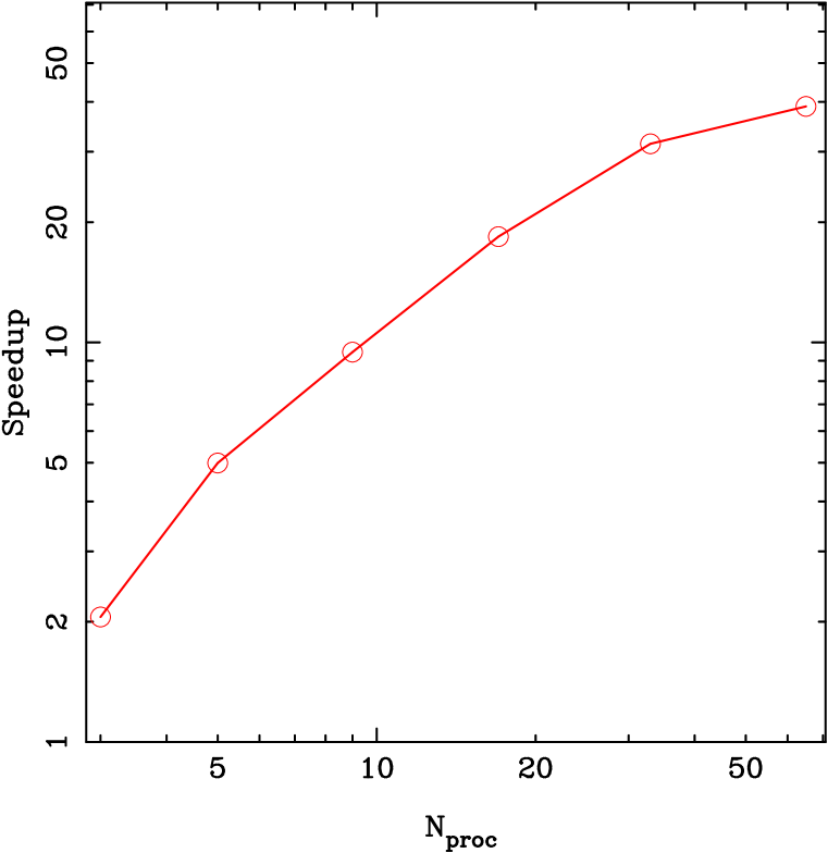
Figure 1: The speedup is plotted here as a function of $N_{proc}$ for a $128^{3}$ simulation (circles). Features expected from the analysis of the algorithm are clearly seen here with the efficiency dropping off at both the small and the large $N_{proc}$, at large $N_{proc}$ the speedup begins to saturate and for small $N_{proc}$ the speedup decreases very rapidly.

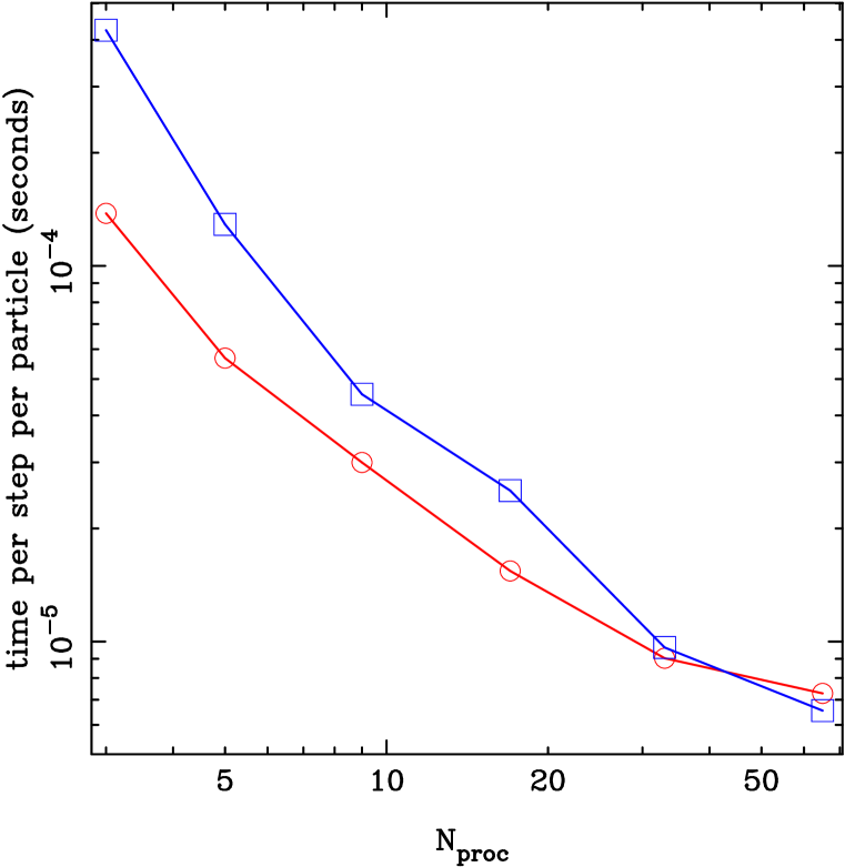
Figure 2: The time taken per step per particle is plotted here as a function of $N_{short}$ for simulations with $128^{3}$ (circles) and $256^{3}$ (squares) particles. Here we have used $N_{long}=1$, thus $N_{proc}=N_{short}+1$. The $256^{3}$ simulation requires about $6.5\mu$s per particle per time step for $N_{proc}=65$.

If we use one processor for long range force calculation while changing $N_{short}$, the number of processors computing the short range force, then speedup will not be linear in $N_{proc}$. For small $N_{short}$, the long range force calculation will take much less time and the efficiency of parallelisation will be low due to poor load balancing. As $N_{short}$ is increased, efficiency of parallelisation will improve till load balancing is achieved. In the regime where $N_{short}$ is smaller than the optimum value for load balancing, the code will speed up faster than linear. For larger $N_{short}$, it will not be possible to load balance as communication overhead and/or long range force calculation will take longer than short range force calculation and there will no significant speed up. The optimum value of $N_{short}$ depends on the size of the simulation and details of how communications are organised. These features can be seen in figure 1 where the speedup is plotted as a function of $N_{proc}$ for $128^{3}$ simulations. The speedup is almost linear beyond $N_{proc}=5$ for simulations with $128^{3}$ particles and it starts dropping beyond $N_{proc}=33$ and the speedup efficiency falls below unity. Data for this figure was obtained on a Linux cluster (Kabir, see http://cluster.mri.ernet.in/ for details) with an SCI (scalable coherent interface) network with computers connected along a $2$d torus. Each node is a dual processor workstation with $2.4$GHz Xeon processors. We obtain a speedup of $31.4$ on $33$ processors and $39$ on $65$ processors for $128^{3}$ simulations. Speedup is greater than the number of processors for $N_{proc}=9$ and $17$, this can be explained in terms of improved cache performance for smaller data sizes.

Performance of the parallel code is presented in fig. 2, where we have plotted time taken per step per particle as a function of $N_{proc}$. Notice that for $N_{proc}=65$, the time taken per step per particle is only $6.5\mu$s for $256^{3}$ simulations, thus we can do a simulation of $4000$ time steps in five days.

We can make further improvement in our method by using more processors for long range force calculation and by using a larger box for computing long range force as this will reduce the communication overhead. These changes, however, will be needed for a larger number of processors that we have access to.

5 Discussion

We have presented an algorithm for parallelising the TreePM code on a Beowulf cluster. This code has been verified by comparing the final positions and velocities of particles in some test cases with the output of the sequential code, therefore the error profile of this code is same as the sequential TreePM code Bagla and Ray (2003). Even though we have tended to optimise the CPU time required at the cost of memory requirements, the maximum memory requirement per node is about $80$ bytes times the number of particles for the double precision code. We need up to $160$ MB per node for $128^{3}$ simulations and $1.25$ GB per node for $256^{3}$ simulations. These numbers represent the maximum memory requirements and for much of the time memory requirement is much smaller than this. Memory requirements can be reduced by about $25\%$ by reorganising the code and adding a master node to gather positions and velocities of particles from nodes that are calculating the short range force.

For $128^{3}$ simulations we get a speedup of $31.4$ on $33$ processors and $39$ on $65$ processors. The time taken for one time step per particle is $6.5\mu$s for a $256^{3}$ particle simulation on $65$ processors, thus a simulation that runs for $4000$ time steps takes $5$ days on this cluster. These results are for a simulation with a global time step and further optimisations in terms of individual time steps is being carried out.

The GOTPM code Dubinski (2004) has a better performance in terms of time taken per particle per step. Part of the speedup is due to use of a larger mesh for the long range force calculation, and the remainder is due to a much smaller $r_{cut}$ and a more relaxed cell acceptance criterion for calculation of the short range force. The results for speedup efficiency and wall clock time per particle compare well with the published numbers for other parallel N-Body simulation codes of this class, e.g., Springel, Yoshida, and White (2001); Bode (2003).

References

- Bagla and Padmanabhan (1997) Bagla J.S. and Padmanabhan T. 1997, Pramana – Journal of Physics 49, 161
- Bagla (2002) Bagla J.S. 2002, Journal of Astrophysics and Astronomy 23, 185
- Bagla (2003) Bagla J.S. 2003, Numerical Simulations in Astronomy, ed. K.Tomisaka and T.Hanawa, p.32
- Bagla and Ray (2003) Bagla, J.S. and Ray, S. 2003, New Astronomy 8, 665
- Barnes and Hut (1986) Barnes J. and Hut P. 1986, Nature 324, 446
- Bernardeau et al. (2002) Bernardeau F., Colombi S., Gaztanaga E. and Scoccimarro R. 2002, Physics Reports 367, 1
- Bertschinger (1998) Bertschinger, E. 1998, ARA&A 36, 599
- Bode (2000) Bode P., Ostriker J.P. and Xu Guohong 2000, ApJS 128, 561
- Bode (2003) Bode P. and Ostriker J.P. 2003, ApJS 145, 1
- Dubinski (1996) Dubinski, John 1996, New Astronomy 1, 133
- Dubinski (2004) Dubinski, John 2004, New Astronomy 9, 111
- Hockney and Eastwood (1988) Hockney R.W. and Eastwood J.W. 1988, Computer Simulation using Particles, (New York: McGraw Hill)
- Knebe, Green and Binney (2001) Knebe A., Green A. and Binney J. 2001, MNRAS 325, 845
- Merz, Pen and Trav (2004) Merz Hugh, Pen Ue-Li and Trac Hy 2004, astro-ph/0402443
- Padmanabhan (1993) Padmanabhan T. 1993, Structure Formation in the Universe, Cambridge University Press
- Peacock (1998) Peacock J.A. 1998, Cosmological Physics, Cambridge University Press
- Peebles (1993) Peebles P.J.E. 1993, An Introduction to Physical Cosmology, Princeton University Press
- Salmon (1991) Salmon, J.K. 1991, PhD Thesis, Parallel Hierarchical N-Body Methods, California Institute of Technology
- Snir et al. (1999) Snir, M., Otto, S., Huss-Lederman, S., Walker, D. and Dongarra, J. 1999, MPI–The Complete Reference. Volume 1, The MPI Core (second edition), MIT Press
- Springel, Yoshida, and White (2001) Springel, V., Yoshida, N. and White, S.D.M. 2001, New Astronomy 6, 79
- Xu (1995) Xu, G. 1995, ApJS 98, 355