Planet Formation by Coagulation: A Focus on Uranus and Neptune

Abstract

Planets form in the circumstellar disks of young stars. We review the basic physical processes by which solid bodies accrete each other and alter each others’ random velocities, and we provide order-of-magnitude derivations for the rates of these processes. We discuss and exercise the two-groups approximation, a simple yet powerful technique for solving the evolution equations for protoplanet growth. We describe orderly, runaway, neutral, and oligarchic growth. We also delineate the conditions under which each occurs. We refute a popular misconception by showing that the outer planets formed quickly by accreting small bodies. Then we address the final stages of planet formation. Oligarchy ends when the surface density of the oligarchs becomes comparable to that of the small bodies. Dynamical friction is no longer able to balance viscous stirring and the oligarchs’ random velocities increase. In the inner-planet system, oligarchs collide and coalesce. In the outer-planet system, some of the oligarchs are ejected. In both the inner- and outer-planet systems, this stage ends once the number of big bodies has been reduced to the point that their mutual interactions no longer produce large-scale chaos. Subsequently, dynamical friction by the residual small bodies circularizes and flattens their orbits. The final stage of planet formation involves the clean up of the residual small bodies. Clean up has been poorly explored.

1 Introduction

The subject of planet formation is much too large for a short review. Our coverage is selective. For a broader perspective, the reader is encouraged to peruse other reviews (e.g., K02; Lis93; Lissauer et al. 1995; Lissauer 2004; S72; Wuchterl, Guillot & Lissauer 2000). Except for a description of gravitational instabilities in cold disks in Section 15.2, we bypass the crucial stage during which dust grains accumulate to form planetesimals. Our story begins after planetesimals have appeared on the scene. Moreover, we focus on processes that occur in gas-free environments. These were likely relevant during the later stages of the growth of Uranus and Neptune.

We devote the first half of the review to the basic physical processes responsible for the evolution of the masses and velocity dispersions of bodies in a protoplanetary disk. Rather than derive precise formulae governing the rates of these processes, we motivate approximate expressions that capture the relevant physics and refer the reader to more complete treatments in the literature (BP90; DT93; Greenberg et al. 1991; Greenberg & Lissauer 1990, 1992; HN90; Hornung, Pellat & Barge 1985; IN89; Oht99; Ohtsuki, Stewart & Ida 2002; Rafikov 2003a,b,d; SI00 ; Stewart & Wetherill 1988). Most of the basic physical processes are, by now, well understood as the result of extensive analytical and numerical investigations by many workers. The velocity dispersion in the shear dominated regime is a notable exception, and here we contribute something new.

The second half of the review is concerned with the growth of planets starting from a disk of planetesimals. Readers not interested in the derivations of equations describing mass and velocity evolution can skip directly to the second half (beginning with Section 6). Although many of our results are general, we concentrate on the formation of the outer planets, Uranus and Neptune. We make this choice for two reasons: The formation of Neptune and Uranus presents the most severe timescale problem. Yet it might be the simplest because it was probably completed in the absence of a dynamically significant amount of gas. Order-of-magnitude estimates, particle-in-a-box simulations, and direct N-body simulations have been used to address this problem. We briefly review the weaknesses and strengths of each approach. Then we show how the simplest of these, the two-groups approximation, can capture many of the results obtained in more sophisticated treatments. We show that the evolution of the mass spectrum can be either orderly, neutral, or runaway and describe oligarchy. We conclude with a discussion of how the Solar System evolved from its state at the end of oligarchy to its present state.

2 The Hill Sphere

For clarity, we consider interactions between two sets of bodies: big ones (protoplanets or embryos) with mass $M$ and small ones (planetesimals) with mass $m$. See Table 1 for a list of symbols. Small bodies have random velocity $u$, i.e., eccentricity $\sim u/\Omega a$, and big bodies have random velocity $v$. We assume, unless explicitly stated otherwise, that inclinations are comparable to eccentricities, in which case the small and big bodies have vertical scale heights $u/\Omega$ and $v/\Omega$, respectively. We also assume that $v<u$, unless stated otherwise (e.g., in Section 5.5).

2.1 Hill Radius, $R_{H}$, and Hill Velocity, $v_{H}$

Planetary accretion calls into play a number of special solutions to the restricted three-body problem. An important system consists of the Sun, a big body, and a small body. The Sun has mass and radius $M_{\odot}$ and $R_{\odot}$, the big body has mass and radius $M$ and $R$, and the small body is here treated as a massless test particle. If the small body is close enough to the big body, then the Sun’s tidal gravitational field is negligible relative to that of the big body. Conversely, if the small body is far enough away, then the big body’s gravitational field is negligible relative to that of the Sun. The Hill radius, $R_{H}$, is the characteristic distance from the big body that distinguishes between these two behaviors. At a distance $R_{H}$, the orbital frequency around the big body is comparable to the orbital frequency of the big body around the Sun, i.e., $(GM/R_{H}^{3})^{1/2}\sim(GM_{\odot}/a^{3})^{1/2}\sim\Omega$, where $a$ is the distance to the Sun. Therefore, $R_{H}\sim a(M/M_{\odot})^{1/3}$, or

$$R_{H}\sim R/\alpha\ ,$$ (1)

where

$$\alpha\equiv\left(\rho_{\odot}\over\rho\right)^{1/3}{R_{\odot}\over a}\,\,.$$ (2)

Here $\rho_{\odot}$ and $\rho$ are the mean densities of the Sun and of a solid body, respectively. Because $\rho\approx\rho_{\odot}\approx 1{\,\rm g}{\,\rm cm}^{-3}$, $\alpha$ is the approximate angular diameter of the Sun as seen from distance $a$. From Earth $\alpha\sim 10^{-2}$, and from the Kuiper Belt $\alpha\sim 10^{-4}$. A parameter similar to our $\alpha$ has been used by Dones & Tremaine (1993), Greenzweig & Lissauer (1990), and Rafikov (2003c).

The Hill velocity $v_{H}$ is a characteristic velocity associated with $R_{H}$. It is the orbital velocity around the big body at a distance $R_{H}$, i.e., $v_{H}\sim(GM/R_{H})^{1/2}$ or

$$v_{H}\sim{v_{\rm esc}}\alpha^{1/2}\sim\Omega R_{H}\ .$$ (3)

For $u>v_{H}$, close encounters of small bodies with big ones are well approximated by two-body dynamics, but for $u<v_{H}$, the tidal gravity of the Sun must be taken into account. The former regime is referred to as dispersion dominated and the latter is referred to as shear dominated.

Small bodies that are initially on circular orbits around the Sun (i.e., $u=0$) and pass near a big body show three types of behavior (see figure 1 in Petit & Henon 1986): For impact parameters from the big body less than approximately $R_{H}$, small bodies are reflected in the frame of the big body upon approach and travel on horseshoe orbits. For impact parameters greater than a few times $R_{H}$, they suffer small deflections while passing the big body. For intermediate impact parameters, they enter the big body’s Hill sphere, i.e., the sphere of radius $\sim R_{H}$ around the big body. Inside the Hill sphere, small bodies follow complex trajectories. Most do not suffer physical collisions with the big body and exit the Hill sphere in an arbitrary direction with random velocities of order $v_{H}$.

2.2 Hill Entry Rate When $u<v_{H}$

When $u<v_{H}$, the number of small bodies that enter into a given big body’s Hill sphere per unit time (the Hill entry rate) is an essential coefficient for estimating the rates of evolution discussed in Sections 3 and 4. As long as $u<v_{H}$, the scale height of the disk of small bodies ($u/\Omega$) is smaller than $R_{H}$. So to calculate the rate at which small bodies enter the Hill sphere, we approximate their disk as being infinitely thin. Their entry rate is equal to their number per unit area ($\sigma/m$, where $\sigma$ is their surface mass density) multiplied by $v_{H}R_{H}$, because the Keplerian shear velocity with which small bodies approach the Hill sphere is $\sim v_{H}$ and the range of impact parameters within which small bodies enter the Hill sphere is $\sim R_{H}$. Combining the above terms, we have

$${\rm Hill\ entry\ rate}\sim{\sigma\over m}\Omega R_{H}^{2}\ \ .$$ (4)

3 Collision Rates

Here we calculate the collision rate suffered by a single big body embedded in a disk of small bodies as the entire swarm orbits the Sun. In Section 5, we convert the collision rate to a mass growth rate, $dM/dt$. Because $v<u$, the orbit of the big body around the Sun can be treated as though it were circular ($v=0$). There are four regimes of interest, depending on the value of $u$ (see Figure 1).

3.1 Super-Escape: $u>{v_{\rm esc}}$

For $u>{v_{\rm esc}}$, where ${v_{\rm esc}}$ is the escape speed from the surface of the big body, gravitational focusing is negligible, and the collisional cross section is $R^{2}$, where $R$ is the radius of the big body. We denote the surface mass density of small bodies by $\sigma$, so their volumetric number density is $\sigma\Omega/(mu)$. Thus,

$${\rm collision\ rate}\sim{\sigma\Omega\over mu}R^{2}u={\sigma\Omega\over m}R^{2}\ \ .\ \ u>{v_{\rm esc}}.$$ (5)

The collision rate depends on the surface number density of small bodies because the $u$ dependence of their flux is canceled by that from their scale height.

3.2 Sub-Escape and Super-Hill: ${v_{\rm esc}}>u>v_{H}$

For $u<{v_{\rm esc}}$, gravitational focusing enhances the collisional cross section. The impact parameter $b_{\rm graze}$ with which a small body must approach the big one just to graze its surface is determined as follows: At approach the small body’s angular momentum per unit mass around the big body is $ub_{\rm graze}$; at contact, it is ${v_{\rm esc}}R$. Thus

$$b_{\rm graze}\sim R{{v_{\rm esc}}\over u}\ ,$$ (6)

and the collisional cross section is $b_{\rm graze}^{2}\sim R^{2}({v_{\rm esc}}/u)^{2}$  . Thus gravitational focusing enhances the collision rate given in Equation 5 by $({v_{\rm esc}}/u)^{2}$:

$${\rm collision\ rate}\sim{\sigma\Omega\over m}R^{2}\left({{v_{\rm esc}}\over u}\right)^{2}\ \ ;\ \ {v_{\rm esc}}>u>v_{H}\ .$$ (7)

3.3 Sub-Hill and Not Very Thin Disk: $v_{H}>u>\alpha^{1/2}v_{H}$

For $u<v_{H}$, the gravitational field of the Sun affects the collision rate, and the Keplerian shear affects both entry and exit from the Hill sphere. Greenberg et al. (1991) were the first to derive analytical expressions for the collision rate in this regime. Although based on their findings, our formulae differ slightly: For reasons that we feel are not well-justified, they used the Tisserand radius, whereas we use the Hill radius. The former is smaller than the latter by $\sim(M/M_{\odot})^{1/15}$.

The collision rate is the product of two terms:

$${\rm collision\ rate}\sim({\rm Hill\ entry\ rate})\cdot{\rm P},$$ (8)

where the Hill entry rate (Equation 4) is the rate at which small bodies enter the big body’s Hill sphere and P is the probability that, once inside the Hill sphere, the small body impacts the big body.

We estimate $P$ as follows: A small body that enters the Hill sphere has its random velocity boosted from $u$ to $v_{H}$. Once inside the Hill sphere, if the small body’s impact parameter relative to the big body is less than $b_{\rm graze}\sim R{v_{\rm esc}}/v_{H}$ (see Equation 6), a collision will occur. Based on Equations 1 and 3, $b_{\rm graze}\sim\alpha^{1/2}R_{H}$, so $b_{\rm graze}<R_{H}$. We now consider the case in which $b_{\rm graze}$ is also smaller than the scale height of small bodies, $u/\Omega$, i.e.,

$$u>\alpha^{1/2}v_{H}\ .$$ (9)

Although we can consider the disk of small bodies to be infinitely thin when calculating the Hill entry rate, we must account for its finite thickness when calculating the collision probability $P$. Because the small bodies’ trajectories within the Hill sphere are random, we estimate $P$ as the ratio of the collisional cross section ($b_{\rm graze}^{2}$) to the cross section of the portion of the Hill sphere that lies within the disk of small bodies ($R_{H}u/\Omega$) (see Figure 1). We obtain

$$P\sim{R_{H}^{2}\alpha\over R_{H}u/\Omega}\sim\alpha{v_{H}\over u}\ \ ,\ \ v_{H}>u>\alpha^{1/2}v_{H}\ .$$ (10)

Inserting Equations 4 and 10 into Equation 8, we find

$${\rm collision\ rate}\sim{\sigma\Omega\over m}R^{2}\alpha^{-1}{v_{H}\over u}\ \ ;\ \ v_{H}>u>\alpha^{1/2}v_{H}\ .$$ (11)

3.4 Very Thin Disk: $u<\alpha^{1/2}v_{H}$

For $u<\alpha^{1/2}v_{H}$, the calculation proceeds as described above, except that the disk of small bodies is considered infinitely thin in the estimation of $P$ (Greenberg et al. 1991, Dones & Tremaine 1993). Thus $P$ is the ratio of the linear range of impact parameters leading to collision ($b_{\rm graze}\sim R_{H}\alpha^{1/2}$) to $R_{H}$; i.e.,

$$P\sim\alpha^{1/2}\ \ ,\ \ u<\alpha^{1/2}v_{H}\ .$$ (12)

Inserting this into Equation 8 and making use of Equation 4 yields

$${\rm collision\ rate}\sim{\sigma\Omega\over m}R^{2}\alpha^{-3/2}\ \ ;\ \ u<\alpha^{1/2}v_{H}\ .$$ (13)

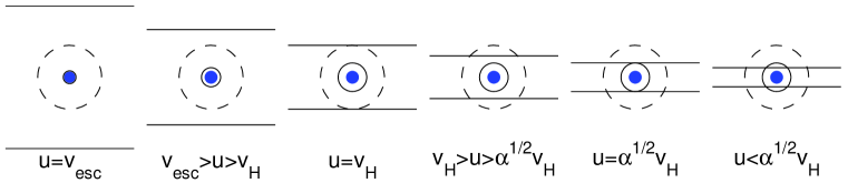
Figure 1: Geometry of disk scale height (solid horizontal line), body size (filled circle), its Hill sphere (dashed circle), and its effective size for accretion (solid circle)

4 Velocity Evolution

Random velocities of big and small bodies, $v$ and $u$, evolve through three processes: cooling by dynamical friction, heating by dynamical friction, and viscous stirring. Terms that promote equipartition of random kinetic energies (dynamical friction) may be separated from those that, in the absence of dissipation, increase random kinetic energies (viscous stirring). In astrophysics, dynamical friction conventionally refers to the cooling term only. To avoid confusion, we always use the modifiers cooling and heating to refer to each effect separately. It is the combination of cooling and heating by dynamical friction that promotes equipartition.

In addition to our usual assumptions, that $u>v$ and $m<M$, we also require that $mu<Mv$. This ensures that a big body will collide with many small bodies before its velocity changes significantly; otherwise, a single collision would suffice. Although it is simple to consider $mu>Mv$ as well, we do not because it is less applicable to protoplanetary disks.

In this section, we quantify the rates of cooling and heating by dynamical friction between groups of bodies with different masses. We do the same for heating by viscous stirring. Unlike dynamical friction, viscous stirring also increases the total energy within a group of homogeneous bodies. We evaluate this in Section 5.2.1. In the following, separate subsections are devoted to the different velocity regimes: $u>{v_{\rm esc}}$, ${v_{\rm esc}}>u>v_{H}$, $u<v_{H}$. The most important results are gathered in Section 5.

4.1 Super-Escape: $u>{v_{\rm esc}}$ and Elastic Collisions

For $u>{v_{\rm esc}}$, gravitational focusing is negligible, and $v$ and $u$ change only when bodies collide. We assume elastic collisions and neglect fragmentation because our aim is to develop intuition applicable to collisionless gravitational scatterings (described below). This case is simple, yet it illustrates how energy is transferred between big and small bodies.

4.1.1 $dv/dt$ due to Dynamical Friction Cooling and Heating

A big body that suffers a head-on collision with a small body loses $\sim m(u+v)$ of its momentum. Because the head-on collision rate is $\sim n_{s}R^{2}(u+v)$, where $n_{s}$ is the number density of small bodies, the big body loses momentum at the rate

$$M{dv\over dt}\Big{|}_{\rm head-on}\sim-n_{s}R^{2}m(u+v)^{2}$$ (14)

as a result of such collisions. Conversely, it gains momentum at the rate

$$M{dv\over dt}\Big{|}_{\rm tail-on}\sim+n_{s}R^{2}m(u-v)^{2}\$$ (15)

owing to tail-on collisions. Combining these two expressions, we find

$${1\over v}{dv\over dt}\Big{|}_{\rm df\ cool}\sim-n_{s}uR^{2}{m\over M}\$$ (16)

to lowest order in $v$. Therefore the big body slows down in the time that it collides with a mass $M$ of small bodies.

If the big body is sufficiently slow, small bodies tend to speed it up. Each scattering with a small body transfers some momentum to the big body, with roughly fixed amplitude ($\sim mu$) and random orientation, so the momentum of the big body increases as in a random walk. After $N$ scatterings, the momentum of the big body grows to $N^{1/2}mu$. The speed $v$ of the big body doubles when $N^{1/2}mu\sim Mv$, i.e., after $N\sim(Mv/mu)^{2}$ scatterings. Thus

$${1\over v}{dv\over dt}\Big{|}_{\rm df\ heat} \sim n_{s}uR^{2}\Big{(}{mu\over Mv}\Big{)}^{2}$$ (17)

$$= -{mu^{2}\over Mv^{2}}\cdot{1\over v}{dv\over dt}\Big{|}_{\rm df\ cool}\ .$$ (18)

Hence $dv/dt|_{\rm df\ cool}+dv/dt|_{\rm df\ heat}=0$ when $Mv^{2}=mu^{2}$. As expected from thermodynamics, dynamical friction drives the big body to equipartition with the small bodies.

In most of our applications, big bodies have higher energies than do small ones so dynamical friction cooling dominates dynamical friction heating.

4.1.2 $du/dt$ due to Dynamical Friction Cooling and Heating

A small body is heated because it gains more energy in head-on collisions than it loses in tail-on ones. It gains energy in head-on collisions at the rate $du^{2}/dt|_{\rm head-on}\sim n_{b}R^{2}(u+v)[(u+2v)^{2}-u^{2}]$, where $n_{b}$ is the number density of big bodies. It loses energy in tail-on collisions at the rate $du^{2}/dt|_{\rm tail-on}\sim n_{b}R^{2}(u-v)[(u-2v)^{2}-u^{2}]$. Adding the two rates, we get

$${1\over u}{du\over dt}\Big{|}_{\rm df\ heat}\sim n_{b}{v^{2}\over u}R^{2}\$$ (19)

to lowest order in $v/u$.

A small body is cooled by a sea of big bodies that are nearly stationary ($v\sim 0$) because the small body loses energy in each collision owing to the recoil of the big body. Because the big body recoils by $\Delta v\sim um/M$, its energy gain is $\sim M(\Delta v)^{2}\sim(um)^{2}/M$, which is equal to the energy lost by the small body. Thus $mdu^{2}/dt|_{\rm df\ cool}\sim-n_{b}uR^{2}(um)^{2}/M$, or

$${1\over u}{du\over dt}\Big{|}_{\rm df\ cool}\sim-n_{b}uR^{2}{m\over M}\ .$$ (20)

Because dynamical friction conserves energy, we could also have used detailed balance,

$$mn_{s}{du^{2}\over dt}\Big{|}_{\rm df\ heat\ or\ cool}=-Mn_{b}{dv^{2}\over dt}\Big{|}_{\rm df\ cool\ or\ heat}\ ,$$ (21)

to derive Equations 19 and 20. However, this approach is less physically enlightening.

4.1.3 Viscous Stirring

Random kinetic energy is not conserved in a circumsolar disk. Viscous stirring tends to increase the random energies of all bodies. This is similar to the way a viscous fluid undergoing shear converts free energy associated with the shear into thermal energy through viscosity. In a circumstellar disk, the shear,$a|d\Omega/da|=3\Omega/2$, is Keplerian. However, for protoplanets and planetesimals the fluid analogy is imprecise because the collision rates are much smaller than the rate of shear.

We consider first how a sea of big bodies moving on circular orbits viscously stirs a small body as it travels around the Sun. Relative to a circular orbit, the small body’s azimuthal and radial speed are of order $u$. An elastic collision rotates the relative velocity vector while preserving its length. That such rotation tends to increase the random energy of the small body can be understood as follows (S72): A body’s speed relative to a cospatial particle moving on a circular orbit is twice as large at quadrature as it is at either periapse or apoapse. Collisions that occur when the small body is at quadrature, and rotate its orbit so that immediately after the collision the small body is at periapse or apoapse, double the epicyclic amplitude. Those collisions that occur when the small body is at periapse or apoapse and rotate its orbit so that the small body is at quadrature halve the epicyclic amplitude. Thus the former increase the random kinetic energy by a factor of four and the latter reduce it by the same factor. Safronov (1972) assumed an equal number of collisions in each direction, which leads to an average increase in random kinetic energy per collision by the factor $(4+1/4)/2=17/8$. His assumption, while quantitatively imprecise, captures the essence of viscous stirring, and implies that the heating rate from viscous stirring is similar to the collision rate:

$${1\over u}{du\over dt}\Big{|}_{\rm vs}\sim n_{b}uR^{2}\ .$$ (22)

Similarly, a big body is viscously stirred by a sea of small bodies in the time it takes for collisions to deflect the big body’s epicyclic velocity by an order-unity angle away from that body’s unperturbed motion. Because this time is the same as that required for $v$ to double by dynamical friction heating, the viscous stirring rate for the big body is the same as its dynamical friction heating rate

$${1\over v}{dv\over dt}\Big{|}_{\rm vs}\sim{1\over v}{dv\over dt}\Big{|}_{\rm df\ heat}\sim n_{s}uR^{2}\Big{(}{mu\over Mv}\Big{)}^{2}\ ,$$ (23)

where the last equality follows from Equation 17.

4.1.4 Collected Results for Elastic Collisions with $u>{v_{\rm esc}}$

The big bodies’ velocity dispersion, $v$, is affected by the small bodies through dynamical friction cooling (Equation 16) and heating (Equation 17), and viscous stirring (Equation 23):

$${1\over v}{dv\over dt}\Big{|}_{\rm df\ cool} \sim -\Omega{\sigma\over\rho R}$$ (24)

$${1\over v}{dv\over dt}\Big{|}_{\rm df\ heat}\sim{1\over v}{dv\over dt}\Big{|}_{\rm vs} \sim \Omega{\sigma\over\rho R}{mu^{2}\over Mv^{2}}\ ,$$ (25)

where we have replaced $n_{s}$ with $\sigma\Omega/(mu)$. Cooling acts in the time that it takes the big body to collide with a mass $M$ of small bodies. The time needed by heating and viscous stirring to act is longer by $Mv^{2}/mu^{2}$.

The small bodies’ velocity dispersion, $u$, is significantly affected by the big bodies only through viscous stirring (Equation 22), which acts in the time that it takes a small body to collide with a big body:

$${1\over u}{du\over dt}\Big{|}_{\rm vs}\sim\Omega{\Sigma\over\rho R}\ ,$$ (26)

where we have replaced $n_{b}$ with $\Sigma\Omega/(Mu)$. Although the number density of big bodies in the midplane is $\Sigma\Omega/(Mv)$, the scale height of the small bodies is larger than that of the big bodies by $u/v$. Thus the effective number density of big bodies, when interactions with small bodies are involved, is smaller than their midplane number density by $v/u$. Heating and cooling of $u$ by dynamical friction (Equations 19 and 20) are less important than viscous stirring by the factors $v^{2}/u^{2}<1$ and $m/M<1$, respectively, so it is safe to neglect them.

4.2 Velocity Evolution when ${v_{\rm esc}}>u>v_{H}$

For $u<{v_{\rm esc}}$, gravitational focusing is important. The principal exchange of momentum between big and small bodies is by collisionless gravitational deflections. A small body that passes within a distance $\sim GM/u^{2}\sim R({v_{\rm esc}}/u)^{2}$ of the big body is deflected by an angle of order unity. Therefore the effective cross section for momentum exchange is $R^{2}({v_{\rm esc}}/u)^{4}$, not $R^{2}$. Appropriate rates are obtained by multiplying Equations 24–26 by $({v_{\rm esc}}/u)^{4}$:

$${1\over v}{dv\over dt}\Big{|}_{\rm df\ cool}\sim-\Omega{\sigma\over\rho R}\left({{v_{\rm esc}}\over u}\right)^{4}\,\,,$$ (27)

$${1\over v}{dv\over dt}\Big{|}_{\rm df\ heat}\sim{1\over v}{dv\over dt}\Big{|}_{\rm vs}\sim\Omega{\sigma\over\rho R}{m\over M}\left(v_{\rm esc}^{2}\over u\,v\right)^{2}\,\,,$$ (28)

$${1\over u}{du\over dt}\Big{|}_{\rm vs}\sim\Omega{\Sigma\over\rho R}\left({{v_{\rm esc}}\over u}\right)^{4}\,\,$$ (29)

(see Appendix D for a more complete derivation of Equation 27). As noted in Section 4.1.4, we can neglect dynamical friction by big bodies on small bodies.

4.3 Velocity Evolution when $u<v_{H}$

Small bodies enter the Hill sphere of a given big body at the rate given by Equation 4 and exit with random velocities $\sim v_{H}$. A big body is cooled by dynamical friction when it strongly scatters a mass $M$ of small bodies (see Section 4.1.1):

$${1\over v}{dv\over dt}\Big{|}_{\rm df\ cool}\sim-{\sigma\over m}\Omega R_{H}^{2}{m\over M}\sim-\Omega{\sigma\over\rho R}{1\over\alpha^{2}}\ .$$ (30)

A big body is heated by viscous stirring when small bodies deflect its random velocity by an angle of order unity. Provided $mv_{H}<Mv$, this occurs after $N\sim(Mv/mv_{H})^{2}$ small bodies enter the big body’s Hill sphere (see Section 4.1.1). Therefore

$${1\over v}{dv\over dt}\Big{|}_{\rm vs}\sim{\sigma\over m}\Omega R_{H}^{2}\Big{(}{mv_{H}\over Mv}\Big{)}^{2}\sim\Omega{\sigma\over\rho R}{1\over\alpha^{2}}{mv_{H}^{2}\over Mv^{2}}\ .$$ (31)

Out of the total momentum transfered in a strong scattering of a small body by a big one, $\sim mv_{H}$ contributes to viscous stirring of the big body and $mu$ to its dynamical friction heating. Thus the dynamical friction heating rate is smaller than the viscous stirring rate by the factor $(u/v_{H})^{2}$ and can be neglected. This result is peculiar to the case $u<v_{H}$. For $u>v_{H}$, the rates of dynamical friction heating and viscous stirring are equal, independent of whether $u<{v_{\rm esc}}$ or $u>{v_{\rm esc}}$.

Viscous stirring of small bodies for $u<v_{H}$ involves subtleties that have gone unrecognized until recently (Rafikov 2003e). For all other processes that we consider, it suffices to leave the definition of $u$ imprecise, but for viscous stirring with $u<v_{H}$ it does not. Consider the case that the velocities of all small bodies are much less than $v_{H}$. Then after only a few small bodies have entered the Hill spheres of big bodies—boosting those small bodies’ energies to $mv_{H}^{2}$—there will be a substantial increase in $\overline{u^{2}}$. But the random speed of a typical small body will not have changed. Hence one must specify whether it is the rms speed $(\overline{u^{2}})^{1/2}$ or the speed of a typical body that is of interest. Most applications require the typical speed of a small body, not the rms speed.

We use $u$ to denote the typical speed. The rate at which $u$ increases is then equal to the rate at which the speed of a typical small body is doubled. If $u\ll v_{H}$, a small body that enters a big body’s Hill sphere has its random energy more than doubled. Thus more distant interactions suffice to double $u$. Because encounters with a big body at the impact parameter,

$$b_{\rm scat}\sim\left(v_{H}\over u\right)^{1/2}R_{H}\,\,,$$ (32)

rotate a random velocity vector of magnitude $u$ by a large angle, the viscous stirring rate is

$${1\over u}{du\over dt}\Big{|}_{\rm vs}\sim{\Sigma\over M}\Omega b_{\rm scat}^{2}\sim\Omega{\Sigma\over\rho R}{1\over\alpha^{2}}{v_{H}\over u}\,\,.$$ (33)

We can estimate the rate at which $\overline{u^{2}}$ increases by taking the product of two terms: (a) the rate at which small bodies enter the big bodies’ Hill spheres and (b) the energy boost that a small body receives upon exiting a big body’s Hill sphere ($mv_{H}^{2}$). After dividing by $\overline{u^{2}}$ to obtain the logarithmic rate, this product yields

$${1\over{\overline{u^{2}}}}{d{\overline{u^{2}}}\over dt}\Big{|}_{\rm vs}\sim{\Sigma\over M}\Omega R^{2}_{H}{v_{H}^{2}\over{\overline{u^{2}}}}\sim\Omega{\Sigma\over\rho R}{1\over\alpha^{2}}{v_{H}^{2}\over{\overline{u^{2}}}}\,\,.$$ (34)

This is how viscous stirring is calculated in the literature, where $\overline{u^{2}}\sim u^{2}$ is also assumed (e.g., Goldreich, Lithwick & Sari 2002; Ida 1990; Weidenschilling et al. 1997; Wetherill & Stewart 1993). But this is incorrect because $\overline{u^{2}}>u^{2}$.

Next we deduce the distribution function for the velocities of the small bodies. A small body approaches a big one with an impact parameter $b>R_{H}$ at a relative speed $\sim\Omega b$. Because the duration of the big body’s peak gravitational acceleration, $\sim GM/b^{2}$, is $\sim\Omega^{-1}$ (independent of $b$), the small body receives a velocity kick $\Delta u\sim(R_{H}/b)^{2}v_{H}$. Because encounters with the impact parameter $b$ occur at a rate proportional to $b^{2}$, velocity kicks of order $\Delta u$ occur at a frequency proportional to $(\Delta u)^{-1}$. The distribution function of random velocities mirrors that of the velocity kicks. It consists of a peak at $\sim u$, which contains approximately half the bodies, and a power law tail of slope minus two at higher velocities. Only a small fraction ($\sim u/v_{H}$) of the bodies have velocities of order $v_{H}$, above which the power law is truncated. The most probable and median velocities are both $\sim u$, but the major contribution to the rms velocity comes from near the upper cutoff, $v_{H}$. The rms velocity is related to $u$ by

$$\left(\overline{u^{2}}\right)^{1/2}\sim\left(uv_{H}\right)^{1/2}\,\,,$$ (35)

which implies that the rates of viscous stirring for $\overline{u^{2}}$ and $u$ are comparable.

4.4 Inclinations and Eccentricities Can Differ

Thus far, our derivations have included the implicit assumption that inclinations and eccentricities have comparable magnitudes. Here we relax this assumption and compare the rates of growth of inclination and eccentricity during viscous stirring. Our concern is with typical, as opposed to rms, values of inclination and eccentricity in the sense described in Section 4.3. Working with the vertical and total components of the random velocity, $u_{\perp}$ and $u$, we assume $u_{\perp}<u$ and compare the excitation rates of each. We then determine whether the growth of $u_{\perp}$ is able to keep pace with that of $u$.

4.4.1 $u<v_{H}$

As shown in Section 4.3, viscous stirring of $u$ is most effectively accomplished by scatterings at impact parameter $b_{\rm scat}$ (Equation 32). On average, each scattering approximately doubles $u$. Because vertical oscillations of the small body carry it a distance of order $u_{\perp}/\Omega$ away from the orbit plane of the large body, these scatterings produce vertical impulses of magnitude $\Delta u_{\perp}$, where

$${\Delta u_{\perp}\over u_{\perp}}\sim{u\over\Omega b_{\rm scat}}\sim\left(u\over v_{H}\right)^{3/2}<1\,\,.$$ (36)

Doubling of $u_{\perp}$ is accomplished most rapidly by closer encounters with $b\sim R_{H}$. Because the scattering rate varies as $b^{2}$, the growth rate of $u_{\perp}$ is slower than that of $u$ according to

$${1\over u_{\perp}}{du_{\perp}\over dt}\sim\left(u\over v_{H}\right){1\over u}{du\over dt}\,\,.$$ (37)

4.4.2 $u>v_{H}$

Strong scatterings for $u>v_{H}$ occur at the impact parameter

$$b_{\rm scat}\sim\left(v_{H}\over u\right)^{2}R_{H}\,\,.$$ (38)

On average, each scattering approximately doubles $u$. Their effect on $u_{\perp}$ differs according to whether the vertical excursion $u_{\perp}/\Omega$ is less than or greater than $b_{\rm scat}$.

In the former case, the scattering takes place when the vertical displacement of the small body is of order $u_{\perp}/\Omega$:

$${\Delta u_{\perp}\over u_{\perp}}\sim{u\over\Omega b_{\rm scat}}\sim\left(u\over v_{H}\right)^{3}>1\,\,.$$ (39)

In the latter case, the small body’s vertical displacement when it scatters is of the same order as $b_{\rm scat}$ so

$${\Delta u_{\perp}\over u_{\perp}}\sim{u\over u_{\perp}}>1\,\,.$$ (40)

In both cases, strong scatterings result in $\Delta u_{\perp}/u_{\perp}>1$. This implies that the growth of $u_{\perp}$ is dominated by more frequent but weaker scatterings. Thus for $u>v_{H}$, the growth of $u_{\perp}$ is faster than that of $u$, provided $u_{\perp}<u$.

5 Mass and Velocity Evolution: Summary and Extensions

5.1 Collected Equations for $u<v_{\rm esc}$

A big body accretes small ones that suffer inelastic collisions with it at $u<v_{\rm esc}$. The big body’s mass growth rate is $m$ times the collision rate. Collecting Equations 7, 11, and 13, we arrive at

$${1\over M}{dM\over dt}\sim{1\over R}{dR\over dt}\sim\Omega{\sigma\over\rho R}F^{col}\left(u\over v_{esc}\right),$$ (41)

where

$$F^{col}(x)=\cases{x^{-2}\ ,&{$1>x>\alpha^{1/2}$}\cr\alpha^{-1/2}x^{-1}\ ,&{$\alpha^{1/2}>x>\alpha$}\cr\alpha^{-3/2}\ ,&{$\alpha>x$} .}$$ (42)

Small bodies are viscously stirred by big ones at the rate (Equations 29 and 33)

$${1\over u}{du\over dt}\Big{|}_{\rm vs}\sim\Omega{\Sigma\over\rho R}F^{vs}\left(u\over v_{esc}\right),$$ (43)

where

$$F^{vs}(x)=\cases{x^{-4}\ ,&{$1>x>\alpha^{1/2}$}\cr\alpha^{-3/2}x^{-1}\ ,&{$\alpha^{1/2}>x$} .}$$ (44)

Dynamical friction heating and cooling of $u$ by big bodies is always negligible relative to viscous stirring.

Big bodies are cooled by small ones at the rate (Equations 27 and 30)

$${1\over v}{dv\over dt}\Big{|}_{\rm df\ cool}\sim-\Omega{\sigma\over\rho R}F^{df}\left({u\over v_{\rm esc}}\right),$$ (45)

where

$$F^{df}(x)=\cases{x^{-4}\ ,&{$1>x>\alpha^{1/2}$}\cr\alpha^{-2}\ ,&{$\alpha^{1/2}>x$} .}$$ (46)

They are viscously stirred by small ones at the rate (Equations 28 and 31)

$${1\over v}{dv\over dt}\Big{|}_{\rm vs}\sim\Omega{\sigma\over\rho R}{mu^{2}\over Mv^{2}}\cases{(u/v_{\rm esc})^{-4}\ ,&{$1>u/v_{\rm esc}>\alpha^{1/2}$}\cr\alpha^{-1}(u/v_{\rm esc})^{-2}\ ,&{$\alpha^{1/2}>u/v_{\rm esc}$} .}$$ (47)

For applications in this review, viscous stirring by big bodies dominates that by small bodies. In general, it is always safe to neglect dynamical friction heating of big bodies by small ones. When $u>v_{H}$, dynamical friction heating is comparable to viscous stirring; when $u<v_{H}$, it is less than viscous stirring.

In deriving these equations, we made the following main assumptions: $v<u$, $mu<Mv$, $u<a\Omega$, $u<v_{\rm esc}$, and inclinations are comparable to eccentricities. We also only considered how big bodies affect small ones, and vice versa, but not how either group affects itself. In the following subsections, we extend these results to cover more general cases.

5.2 How Bodies Affect Themselves

5.2.1 Interactions Among Big Bodies

Expressions for interactions among big bodies are obtained by replacing $u$ by $v$ and $\sigma$ by $\Sigma$. Thus big bodies coalesce at the rate (Equation 41)

$${1\over R}{dR\over dt}\sim\Omega{\Sigma\over\rho R}F^{col}\left({v\over v_{\rm esc}}\right)\ \ ,\ \ \ \ \ v<v_{\rm esc}$$ (48)

and stir themselves at the rate (Equation 43)

$${1\over v}{dv\over dt}\Big{|}_{\rm vs}\sim\Omega{\Sigma\over\rho R}F^{vs}\left({v\over v_{\rm esc}}\right)\ \ ,\ \ \ \ \ v<v_{\rm esc}\ .$$ (49)

Dynamical friction, in the collective manner we use it, drives two groups to equipartition with each other; it does not act within a single group of homogeneous bodies.

5.2.2 Inelastic Collisions Among Small Bodies

It suffices to consider the case $u>u_{\rm esc}$ for which gravitational focusing is unimportant. In Section 4.1, we assume for pedagogical reasons that physical collisions are perfectly elastic, in which case small bodies viscously stir themselves when they collide. However, real collisions are inelastic. They damp $u$ in a collision time:

$${1\over u}{du\over dt}\sim-\Omega{\sigma\over\rho s}\ \ ,\ \ \ \ \ u>u_{\rm esc}\ ,$$ (50)

where $s$ is the radius of a small body. Inelastic collisions damp $u$ provided the coefficient of restitution falls below a critical value (0.63 in the idealized model of Goldreich & Tremaine 1978). Above the critical value, the net effect of collisions is to increase $u$. When $u<u_{\rm esc}$, strong gravitational interactions are more frequent than collisions, and they cause $u$ to increase. When $u\gg u_{\rm esc}$, collisions fragment small bodies that have little cohesive strength. We explore the implications of fragmentation in subsequent sections.

5.3 Effect of Anisotropic Velocities on the Accretion Rate

For $v<v_{H}$, the big bodies’ inclination growth by viscous stirring is slower than their eccentricity growth (see Section 4.4). As discussed below, the velocity dispersion of large bodies is set by the balance between mutual eccentricity excitation and dynamical friction from small bodies. Because dynamical friction acts on the horizontal and vertical velocity with comparable timescales, inclinations are damped faster than they are excited. Large bodies with $v<v_{H}$ lie in a flat disk. Thus the vertical thickness of the disk of large bodies varies discontinuously across $v\sim v_{H}$. This has one profound consequence: A flat disk enhances the focusing factor for mutual collisions of large bodies across $v\sim v_{H}$. So big bodies grow by accreting each other at a rate given by inserting

$$F^{col}(x)=\cases{x^{-2}\ ,&{$1>x>\alpha^{1/2}$}\cr\alpha^{-3/2}\ ,&{$x<\alpha^{1/2}$}\cr}$$ (51)

into Equation 48 (instead of inserting Equation 42). Similarly, collisionless small bodies with $u<v_{H}$ lie in a flat disk. So big bodies grow by accreting them at a rate given by inserting Equation 51 for $F^{col}$ into Equation 41. But if small bodies collide frequently, they isotropize their velocity dispersion, in which case Equation 42 for $F^{col}$ is applicable.

The flattening of a shear-dominated disk has largely been neglected in the literature. Wetherill & Stewart (1993) and Weidenschilling et al. (1997) discovered it in numerical simulations, and Rafikov (2003e) provided a simple explanation similar to ours.

5.4 Mass Evolution for $u>v_{\rm esc}$

Gravitational focusing does not operate when $u>v_{\rm esc}$, so the collision cross section is $R^{2}$. An upper limit to the growth rate of big bodies is obtained by adding the mass of the impacting small bodies to that of the big body: Equation 5 yields

$${1\over R}{dR\over dt}\sim\Omega{\sigma\over\rho R}\ \ ,\ \ \ \ \ u>v_{\rm esc}\ .$$ (52)

However, fragmentation of the material composing the bodies may result in net mass loss from the big body, especially if $u\gg v_{\rm esc}$.

5.5 Physical Processes when $v>u$

We consider first the case that $v_{\rm esc}>v>v_{H}$. Because the relative speed between big and small bodies is $v$, it is $v$ that enters into the gravitational focusing factor for accretion. Thus the accretion rate is given by Equation 41 with $u$ replaced by $v$, i.e., $(1/M)dM/dt\sim(\sigma\Omega/\rho R)(v_{\rm esc}/v)^{2}$. For viscous stirring of small bodies by big ones, a small body is deflected by $u$ when it passes within a distance $R(v_{\rm esc}^{2}/uv)$ of a big one. So the cross section for viscous stirring differs from that used in Equation 43 by the multiplicative factor $u^{2}/v^{2}$, and $(1/u)du/dt|_{\rm vs}\sim(\Sigma\Omega/\rho R)(v_{\rm esc}^{4}/u^{2}v^{2})$. This is comparable to the rate at which $u$ is heated by big bodies via dynamical friction. Cooling of $u$ by dynamical friction with big bodies is negligible, because a big body has more random energy than a small one. Big bodies are cooled by dynamical friction with the small bodies at a rate obtained by replacing $u$ with $v$ in Equation 45: $(1/v)dv/dt|_{\rm df\ cool}\sim-(\sigma\Omega/\rho R)(v_{\rm esc}/v)^{4}$.

When $v<v_{H}$, the big bodies lie in a flat disk (see Section 5.3). If the small bodies were collisionless, their disk would also be flat. We consider instead the more practical situation in which collisions roughly isotropize their velocity distribution. Then there are no differences in the important rates of accretion, viscous stirring, and dynamical friction between the case $u<v<v_{H}$ and the one considered previously, i.e., $v<u<v_{H}$. In both cases, the rate at which big and small bodies approach each other is independent of $u$ or $v$ and set by the Keplerian shear. The mass accretion rate is given by Equation 41, viscous stirring of small bodies is given by Equation 43, and dynamical friction of big bodies is given by Equation 45. The accretion rate is discontinuous across $v=v_{H}$ for $u<v_{H}$.

5.6 Derivations of Mass and Velocity Evolution: Some Highlights

The book by Safronov (1972) contains the first systematic treatment of mass and velocity evolution in protoplanetary disks. It provides approximate expressions for mass evolution, viscous stirring, and dynamical friction drag, but primarily for ${v_{\rm esc}}>u>v_{H}$. Greenberg et al. (1991) derived analytic formulae for mass accretion for $u<v_{H}$. Dones & Tremaine (1993) found order-unity coefficients when $u=0$ by performing numerical integrations.

Numerous authors have employed increasingly sophisticated techniques in more precise derivations of the velocity evolution rates for ${v_{\rm esc}}>u>v_{H}$. There are two types of derivations: one based on a Fokker-Planck equation (the local-velocity formalism), and the other based on averaging over orbital elements (the Hill velocity formalism). Stewart & Ida (2000) showed that both formalisms lead to the same results. In the process, they corrected various order-unity errors that had appeared in previous derivations.

Ida (1990) considered velocity evolution when $u<v_{H}$. He used scaling arguments, as well as numerical experiments, for the case $u=0$ to estimate order-unity coefficients. Some of his “order-unity” coefficients are quite large—nearly $10^{2}$. Ohtsuki, Stewart & Ida (2002) compared predictions of analytically derived formulas for dynamical friction and viscous stirring with numerical integrations.

6 Growth of Planets: An Overview

Before solving the mass and velocity evolution equations, we present general arguments about how planets might have formed. These lead us to deduce that Uranus and Neptune grew by accreting small bodies.

6.1 Observational Constraints

In contemplating the formation of Uranus and Neptune, we are guided by a few observational constraints. Foremost among them are the planets’ masses and radii and the age of the Solar System. Gravitational oblatenesses provide more subtle clues. Interior models that fit these data probably require that Uranus and Neptune each contains a few Earth masses of hydrogen and helium Guillot (1999). This would imply that protoplanets sufficiently massive to accrete an envelope of gas must have formed prior to the total loss of the Sun’s protoplanetary gas disk. Observations of young, solar-type stars suggest that circumstellar disks dissipate over a timescale of several million years (Briceño, Vivas & Calvet 2001; Haisch, Lada & Lada 2001; H02; Lagrange, Backman & Artymowicz 2000; Strom, Edwards & Skrutskie 1993).

We ignore other observational clues that deserve further attention. Among these are Uranus’s and Neptune’s residual heat (Hubbard, Podolak & Stevenson 1996; Podolak, Hubbard & Stevenson 1991), as well as their substantial obliquities and nonzero orbital eccentricities and inclinations. Giant impacts are obvious candidates for producing the obliquities, but they are not required: At least for Saturn, a good case can be made for spin-orbit resonances (Hamilton & Ward 2002).

6.2 Minimum Mass Solar Nebula

We adhere to the prevailing view that planets are born in disks around young stars. The minimum mass solar nebula is a useful reference disk Edgeworth (1949); Kuiper (1956); Weidenschilling 1977bb ; Hayashi (1981). Its surface density of condensates is

$$\sigma_{\rm MMSN}\sim\left({a\over 10{\rm\ AU}}\right)^{-3/2}{\,\rm g}{\,\rm cm}^{-2}\ \ ,\ \ a\mathrel{\hbox{\hbox to0.0pt{\hbox{\lower 4.0pt\hbox{$\sim$}}\hss}\hbox{$>$}}}2.7{\rm\ AU}\ \ .$$ (53)

Hayashi (1981) arrived at this expression by imagining that the material in each planet, other than hydrogen and helium, was distributed in an annulus around the planet, such that the annuli of neighboring planets just touch. The minimum mass solar nebula (MMSN) assumes Jupiter, Saturn, Uranus, and Neptune each contributes 15 Earth masses, a value that is consistent with modern interior models Guillot & Gladman (2000). In our numerical expressions, we use the radius

$$R_{\rm planet}\sim 25,000{\,\rm km}$$ (54)

for Uranus and Neptune and for the cores of Saturn and Jupiter.

Throughout this review, our default option is to assume that the surface density of solid bodies is given by the MMSN, although it is conceivable that, initially, it was much greater and that the excess was either ejected from the Solar System or accreted by the Sun. A higher initial surface density might shorten the timescale for planet formation (e.g., Thommes, Duncan & Levison 2003). A possible measure of the initial surface density is given by the Oort cloud because comets that reside there are thought to have formed near the planets, before the planets kicked them out to their present large distances (more than a few thousand astronomical units). The current mass of the Oort cloud is thought to be between 1 and 50 Earth masses Weissman (1996). If one also accounts for the mass that is completely ejected from the Solar System, the MMSN might underestimate the original surface density by an order of magnitude (Dones et al. 2001).

6.3 Need for Gravitational Focusing

If most of the time that it takes a planet to grow is spent in the last doubling of its mass, then its formation time can be estimated from Equation 41, after setting $(1/M)dM/dt\sim 1/t_{\rm form}$:

$$t_{\rm form} \sim \Omega^{-1}{\rho R\over\sigma}\left({u\over v_{\rm esc}}\right)^{2}\ \ \ \ \ v_{H}<u<v_{\rm esc}\ ,$$ (55)

where $u$ is the velocity dispersion of the mass that is accreted during the final stages of its growth. Taking $\sigma$ to be that of the MMSN (Equation 53) and $R$ to be the outer planets’ radii (Equation 54) gives

$$t_{\rm form}\sim 15\left({a\over 10{\,\rm AU}}\right)^{3}\left({u\over v_{\rm esc}}\right)^{2}\ {\rm Gyr}\ .$$ (56)

Without gravitational focusing, i.e., with $u=v_{\rm esc}$, it would have taken Uranus and Neptune 100 Gyr and 400 Gyr, respectively, to form. For Neptune to have formed in the age of the Solar System, it must have accreted material with $u\mathrel{\hbox{\hbox to0.0pt{\hbox{\lower 4.0pt\hbox{$\sim$}}\hss}\hbox{$<$}}}v_{\rm esc}/10$. These estimates are based on the assumption that the outer planets formed from the MMSN at their current distances from the Sun. An alternative scenario is given by Thommes, Duncan & Levison (1999, 2002) , who suggest that Uranus and Neptune formed between Jupiter and Saturn before Jupiter and Saturn accreted gas.

6.4 Cooling Is Necessary, so Accreted Bodies Were Small

A planetary embryo viscously stirs all planetesimals that it significantly deflects. But, provided $u<v_{\rm esc}$, only a small fraction of deflected planetesimals are accreted. This is simply because the cross section for scattering exceeds that for accretion, i.e., $F^{col}(u/v_{esc})<F^{vs}(u/v_{esc})$ when $u<v_{esc}$. Thus an embryo heats its food faster than it can eat it. If the small bodies are not cooled by inelastic collisions or gas drag, only a small fraction of them are accreted while $u<v_{\rm esc}$; most are accreted when $u\sim v_{\rm esc}$. Therefore without cooling, most planetesimals are accreted when gravitational focusing is inoperative, and Uranus and Neptune would have taken far too long to form. These general conclusions are in accord with results from N-body simulations by Levison & Stewart (2001) that follow the evolution of a system initialized with a few hundred equal mass bodies whose total mass slightly exceeds that of Uranus and Neptune combined. These simulations, which also include perturbations from Jupiter and Saturn, find almost no growth in the region of Uranus and Neptune because viscous stirring is faster than accretion. Levison, Lissauer & Duncan (1998) and Levison & Stewart (2001) showed that earlier work arriving at contradictory conclusions Ip (1989); Fernández & Ip (1996); Brunini & Fernández (1999) is incorrect.

How small must the bodies accreted by Neptune have been for them to be cooled by inelastic collisions? Balancing viscous stirring by an embryo (Equation 43 with $\Sigma\sim\sigma$) with inelastic collisions between small bodies of radius $s$ (Equation 50) gives $s/R\sim(u/v_{\rm esc})^{4}$. Because $u\mathrel{\hbox{\hbox to0.0pt{\hbox{\lower 4.0pt\hbox{$\sim$}}\hss}\hbox{$<$}}}v_{\rm esc}/10$ is required for Neptune to have formed in the age of the Solar System, the accreted bodies must have been smaller than a few kilometers. Rafikov (2003e) and Thommes, Duncan & Levison (2003) found protoplanets grow rapidly when they accrete small bodies; Rafikov (2003e) considers the damping of $u$ by gas drag.

Although this review focuses on the formation of Uranus and Neptune, we mention briefly that for Earth, Equation 55 gives $t_{\rm form}\sim 0.1$ Gyr without gravitational focusing. Hence Earth need not have accreted small bodies. Indeed, the Moon is thought to have formed when Earth accreted a body not much smaller than itself Canup & Asphaug (2001).

6.5 Completion: When Small Bodies Have Been Consumed

If the planets formed out of the MMSN, they must have eaten all the condensates in the disk. Uranus and Neptune ate these condensates in the form of bodies smaller than 1 km (Section 6.4). We refer to the epoch when all small bodies have been consumed as completion. Any formation scenario that produces numerous subplanet-size big bodies beyond Saturn’s orbit at completion is unacceptable. Although subplanets might have formed quickly, further significant growth is impossible in the age of the Solar System, because subplanets viscously stir each other faster than they coalesce (see Section 6.4). How could Uranus and Neptune have consumed all small bodies that were between them? In the following, we consider two possibilities.

6.5.1 Completion With $u\sim\Omega a$

The simplest possibility is that the orbits of accreted bodies crossed those of the growing protoplanets as a result of their epicyclic motions. For the accreted bodies’ epicycles to be as large as $a$, they must have had $u/\Omega\sim a$. Of course, $u$ could not have exceeded $a\Omega$, or the bodies would have escaped from the Solar System. With $u\sim\Omega a$, Equation 56 gives

$$t_{\rm form}\sim 2\left({a\over 10{\rm\ AU}}\right)^{2}\ {\rm Gyr}\ ,$$ (57)

i.e., $t_{\rm form}\sim 20$ Gyr for Neptune. Thus the giant planets could barely have formed in the age of the Solar System if $u\sim\Omega a$. But there is a serious problem with this scenario. Small bodies must experience frequent collisions (see Section 6.4), and their sizes must be $\sim 1$ km to keep $u\sim\Omega a$. These collisions would fragment them because $\Omega a\sim$ few kilometers per second greatly exceeds the escape speed from their surfaces, $u_{\rm esc}\sim 1$ m/s. Fragmentation implies smaller bodies, which implies more effective inelastic damping, and hence smaller $u$. This leads us to examine the case $u\ll\Omega a$.

6.5.2 Completion with $u\ll a\Omega$

It is also possible that $u\ll a\Omega$. The accretion time could then easily be less than 10 Myr. However, the epicycles of the accreted bodies would only allow them to accrete onto nearby planetary embryos. For example, if $u\ll v_{H}$, an embryo could only accrete from within its Hill sphere, i.e., within an annulus of half-width $2.5R_{H}$ (Greenberg 1991). The embryo’s maximum radius $R$ is given by $2\pi\sigma a(5R_{H})=(4/3)\pi\rho R^{3}$, where $R_{H}\cong 0.62R(a/R_{\odot})$ and taking $\rho\cong 1{\,\rm g}{\,\rm cm}^{-3}$ for the embryo. Solving for $R$ and setting $\sigma=\sigma_{\rm MMSN}$ yields the Hill isolation radius:

$$R_{\rm iso}\cong 12,000\left({a\over 10{\,\rm AU}}\right)^{1/4}\ {\,\rm km}\$$ (58)

(e.g., Lissauer 1993). At 20–30 AU, the final masses of the isolated embryos would be smaller than Uranus and Neptune (Equation 54) by a factor of $\sim 5$. So if accretion with $u\ll v_{H}$ proceeded to completion, one would expect approximately 10 small planets beyond Saturn.

This conclusion could be avoided if a mechanism other than the small bodies’ epicyclic motions enabled them to travel a distance $a$. For example, small bodies might diffuse a distance $a$ owing to collisions among themselves, or they could drift as a result of gas drag (Weiden77b; Kary, Lissauer & Greenzweig 1993). Alternatively, the planets themselves might migrate (Bryden, Lin & Ida 2000; FIP84; HM99; TI99; Ward89).

An alternative that we regard as most likely is that $\sigma$ was a few times larger than $\sigma_{\rm MMSN}$. Because $R_{\rm iso}\propto\sigma^{1/2}$, this would have produced planets whose radii are equal to those of Uranus and Neptune. But it would have produced half a dozen of them, instead of two. We discuss what happens to the extra planets in Section 11.

We have yet to address how $u\ll v_{H}$ might be maintained. Although cooling by gas drag is a possibility, we favor inelastic collisions because it appears that the final assembly of Neptune took place after most of the gas had dissipated. As seen by equating Equations 43 and 50, collisional cooling requires $s\ll R\alpha^{2}$. For Neptune, this translates into $s<30$ cm. Such small bodies might result from fragmentation.

7 Solving the Evolution Equations

7.1 N-Body and Particle-in-a-Box Simulations

In principle, one could initiate a simulation with many small bodies orbiting the Sun and integrate the equations of motion. However, aside from fundamental uncertainties such as the initial size of the bodies and whether colliding bodies stick or fragment, this approach is computationally impossible. To describe the formation of 25,000-km bodies out of, say, 1-km ones, requires following an astronomical number, $25,000^{3}$, of particles. Nonetheless, N-body simulations can be useful for following the evolution of a few hundred bodies (Cham01; IM92; Kokubo & Ida 1996, 2000; LS01).

An alternative to the N-body approach is to group all bodies with similar masses together and to treat each group as a single entity that has three properties: the number of bodies it contains, the mass per body, and the characteristic random velocity. Each group interacts with every other group (and with itself); groups change each other’s properties at rates that are given by the formulae in Section 5. This particle-in-a-box approach was pioneered by Safronov (1972) and extended by many others (Davis et al. 1985; Greenberg et al. 1978, 1984; Inaba et al. 2001; Kenyon 2002; Kenyon & Bromley 2001; Kenyon & Luu 1998, 1999; Ohtsuki, Nakagawa & Nakazawa 1988; Spaute et al. 1991; Stern & Colwell 1997; Weidenschilling et al. 1997; Wetherill & Stewart 1989, 1993; Wetherill 1990).

Although particle-in-a-box simulations represent a great simplification relative to N-body simulations, they are still computationally expensive (Kenyon & Luu 1998, for example, ran their simulations on a CRAY supercomputer). Moreover, the results of the simulations are very difficult to interpret. Because each group interacts with every other group, it is not clear which groups are important for viscously stirring the others, which are important for dynamical friction, or whether bodies grow primarily by merging with others of comparable size or by accreting much smaller ones. Disentangling these effects is important for understanding planet formation and for assessing how various uncertainties—such as fragmentation and the initial sizes of the bodies—affect the final results.

7.2 Two-Groups Approximation

A further simplification is to consider the evolution of only two groups of bodies: big and small ones (e.g., WS89, IM93). In the remainder of the review, we concentrate on this two-groups approximation. We use the same notation used in Section 5 to refer to the properties of these two groups ($\sigma,u,s,u_{\rm esc},\Sigma,v,R,v_{\rm esc},v_{H}$). Motivated by the results of particle-in-a-box simulations, we define the small bodies as those that both contain most of the mass and provide most of the dynamical friction, and we define the big ones as those that dominate the viscous stirring, even though they may contribute very little to the total mass. The identification of these two groups with the results of numerical simulations depends on the mass and velocity spectra.

We collect the interaction rates summarized in Section 5. Big bodies grow at the rate (Equations 41 and 48)

$${1\over R}{dR\over dt}\sim\Omega{\Sigma\over\rho R}F^{col}\left({v\over v_{\rm esc}}\right)+\Omega{\sigma\over\rho R}F^{col}\left({u\over v_{\rm esc}}\right)\ ,$$ (59)

where $F^{col}$ is given by Equation 51; however, if small bodies experience frequent collisions that isotropize their random velocities, the second term should instead use Equation 42 for $F^{col}$. Random velocities of small and large bodies evolve at the rates (Equations 43, 45, 49, 50)

$${1\over u}{du\over dt} \sim \Omega{\Sigma\over\rho R}F^{vs}\left({u\over v_{\rm esc}}\right)-\Omega{\sigma\over\rho s}$$ (60)

$${1\over v}{dv\over dt} \sim \Omega{\Sigma\over\rho R}F^{vs}\left({v\over v_{\rm esc}}\right)-\Omega{\sigma\over\rho R}F^{df}\left({u\over v_{\rm esc}}\right)\ .$$ (61)

In addition to the assumptions listed at the end of Section 5.1, we also assume that $u>u_{\rm esc}$ and that viscous stirring of big bodies by small ones is negligible. Equations 59–61 are three equations for five unknowns, $R$, $u$, $v$, $s$, and $\Sigma$. The quantities $\Omega$ and $\rho$ are known, and $v_{\rm esc}\sim R(G\rho)^{1/2}\sim\alpha^{-3}R\Omega$. Because initially most of the mass is in small bodies, $\sigma$ does not evolve until $\Sigma$ grows to a comparable value; in numerical estimates, $\sigma$ is set by the minimum mass solar nebula (see Section 6.2).

The left-hand side of Equation 59 represents the inverse of the time at which big bodies—i.e., those bodies that dominate the stirring—have reached radius $R$. One might expect that, if big bodies grow by accreting small ones, then their number should not evolve, i.e., $\Sigma\propto R^{3}$. Similarly, if big bodies grow by accreting each other, one might expect that $\Sigma=$ constant. In general, neither expectation is met. Even if big bodies accrete only each other, or only very small bodies, different subsets of big bodies can dominate the stirring, and thus $\Sigma$, at various times.

How then does $\Sigma$ grow? In Sections 9 and 10, we provide appropriate expressions for $\Sigma$ during oligarchy, an important stage of planet formation. However, at earlier times, $\Sigma$ must be obtained by solving an integro-differential equation (the coagulation equation), which is a difficult task Lee (2000); Malyshkin & Goodman (2001). Although irrelevant for the final stages of planet formation, the value of $\Sigma$ at early times is important for systems that have not yet reached oligarchy, such as the Kuiper Belt, and for determining when oligarchy begins. Numerical simulations have produced contradictory results (Davis, Farinella & Weidenschilling 1999; Inaba et al. 2001; Kenyon & Luu 1998; Lee 2000; Wetherill & Stewart 1993). The observed spectrum of Kuiper Belt objects (Bernstein et al. 2003; Luu & Jewitt 1998; Luu, Jewitt & Trujillo 2000; TB01 ; Trujillo, Jewitt & Luu 2001) may provide a clue, if, as Kenyon & Luu (1999) have proposed, it is a frozen image of the formation epoch. In the following, we treat $\Sigma$ as a free function. Where appropriate, we insert the oligarchic expressions for $\Sigma$.

7.3 Solutions in the Two-Groups Approximation

7.3.1 Overview of Method of Solution

With the aid of physical insight, Equations 59–61 can be reduced to algebraic relations that are trivial to solve. Nonetheless, the algebra is messy, particularly because of the multitude of cases. We outline how to solve the equations before actually solving them. We treat $\Sigma$ as an unknown function and assume $s$ is fixed, either at its initial value or at some as-yet unspecified value. There remain three equations for three unknowns: $v$, $u$, and $R$.

On big bodies, viscous stirring is balanced by dynamical friction, so $v$ is in quasi-steady state and is determined by equating the right hand side of Equation 61 to zero. Two possibilities exist for $u$. If small bodies have had time to collide with each other, then $u$ is in quasi-steady state: Viscous stirring of small bodies by big ones occurs at the same rate as damping by inelastic collisions, so $u$ is given by setting the right-hand side of Equation 60 to zero. If small bodies have not yet collided, the second term on the right-hand side of Equation 60 is negligible. Because the remaining term is proportional to $u$ raised to some power, $u$ increases on timescale $t$ such that $(1/u)du/dt\sim 1/t$ once $u$ has grown to be much larger than its initial value. Equation 59 for $R$ can also be solved by replacing $(1/R)dR/dt$ with $1/t$. We give some explicit solutions below, focusing on a few that have the virtues of relevance and simplicity.

7.3.2 Quasi-Steady State of $v$

The two terms on the right-hand side of Equation 61 are always larger than the corresponding terms on the right-hand side of Equation 59. Viscous stirring acts in the time that a big body is significantly deflected. Similarly, dynamical friction acts in the time that $M/m$ small bodies are significantly deflected. Because only a subset of the deflected bodies are accreted, $v$ achieves a quasi-steady state on a timescale shorter than that at which $R$ grows. Thus

$$\Sigma F^{vs}\left({v\over v_{\rm esc}}\right)\sim\sigma F^{df}\left({u\over v_{\rm esc}}\right)\$$ (62)

gives one relation between $u$, $v$, and $R$.

The evolution equation for $u$ (Equation 60) does not involve $v$. However, $v$ is present in the first term on the right-hand side of the evolution equation for $R$ (Equation 59) which arises from the merging of big bodies. Nevertheless, the value of $v$ does not appear in the solution of Equation 59.

If $v>v_{H}$, then

$$v\sim u\left({\Sigma\over\sigma}\right)^{1/4}\ ,\ \ \ \ \ {v>v_{H}}\ \$$ (63)

and the growth of $R$ due to the accretion of small bodies proceeds faster, by the factor $(\sigma/\Sigma)^{1/2}$, than that due to merging of big bodies. By contrast, Makino et al. (1998) concluded that big bodies grow primarily by merging with other big bodies. But their result was derived under the assumption that the velocities of all bodies follow from energy equipartition, whereas we find a different result (see Equation 63 and Figures 2 and 3).

If $v<v_{H}$, then the disk of big bodies is flat and big bodies accrete each other at the $v$-independent rate $\alpha^{-3/2}\Sigma\Omega/(\rho R)$. Whether embryo growth is dominated by the accretion of big or small bodies can be determined by comparing the two terms in Equation 59 once a solution for $u$ is at hand.

7.3.3 Collisionless Solution with $u>v_{H}$ and $v>v_{H}$

This case is a useful vehicle for comparing our simple analytic solutions with detailed numerical simulations done by Kenyon & Luu (1998, 1999) and Kenyon (2002). It may describe the late stages of accretion in the Kuiper belt. The collisionless limit applies for $t<t_{\rm collide}$, where

$$t_{\rm collide}\sim\Omega^{-1}{\rho s\over\sigma}\sim 0.6\left({a\over 10{\rm\ AU}}\right)^{3}\left({s\over{\rm km}}\right){\,\rm Myr}\ .$$ (64)

is the collision time between small bodies (Equation 60). We use the MMSN value of $\sigma$ (Equation 53) in numerical expressions. When $t<t_{\rm collide}$, the second term on the right-hand side of Equation 60 is negligible. Because big bodies grow by accreting small ones (Section 7.3.2), we drop the first term on the right-hand side of Equation 59. Setting $(1/R)dR/dt\sim(1/u)du/dt\sim 1/t$ in Equations 59 and 60 yields

$${u\over v_{\rm esc}} \sim \left({\Sigma\over\sigma}\right)^{1/2}$$ (65)

$$t \sim \Omega^{-1}{\rho R\over\sigma}{\Sigma\over\sigma}\ .$$ (66)

Given $\Sigma/\sigma$ at time $t$, the above formulae determine $R$ and $u$.

The assumption of super-Hill velocities ($v>v_{H}$) constrains

$${\Sigma\over\sigma}>\alpha^{2/3}\,,$$ (67)

(see Equations 63 and 65), and the restriction to $t<t_{\rm collide}$ constrains

$$s>{\Sigma\over\sigma}R\,$$ (68)

(see Equations 64 and 66).

Next we determine the velocities of intermediate-sized bodies (those with radii $s<R^{\prime}<R$) (see Rafikov 2003d for a more detailed treatment). Bodies of intermediate size are passive; they contribute negligibly to both viscous stirring and dynamical friction. The collisionless case is simplified by its mass-blind aspect: Up to radius $R_{\rm fr}$, at which dynamical friction becomes significant, the velocity dispersion is determined solely by viscous stirring from big bodies. Thus the velocity spectrum is flat between $s$ and $R_{\rm fr}$ (see Figure 2), where $R_{\rm fr}$ is the radius at which dynamical friction damps the random velocity $v^{\prime}$ on timescale $t$:

$$R_{\rm fr}\sim\left(\Sigma\over\sigma\right)^{1/3}R\,.$$ (69)

For consistency, $s$ must be smaller than $R_{\rm fr}$.

For $R_{\rm fr}<R^{\prime}<R$, viscous stirring by the big bodies and dynamical friction from the small ones maintains the random velocity $v^{\prime}$ in quasi-equilibrium at

$$v^{\prime}\sim v_{\rm esc}\left(R\over R^{\prime}\right)^{3/4}\left({\Sigma\over\sigma}\right)^{3/4}\,.$$ (70)

Although $v^{\prime}$ decreases with increasing $R^{\prime}$, the kinetic energy increases proportional to $(R^{\prime})^{3/2}$.

At this stage, we gather our analytic results and provide numerical scalings that may be relevant to the formation of Kuiper belt objects. Motivated by Kenyon’s simulations, we choose the following parameters: $\Sigma/\sigma=0.01$ and $\sigma=0.2{\,\rm g}{\,\rm cm}^{-2}$ at $a=35{\,\rm AU}$. As demanded by Equation 67, $\Sigma/\sigma>\alpha^{2/3}$, so that $v>v_{H}$. From Equation 64, we find that the collisionless approximation applies up to $t_{\rm collide}\sim 20(s/{\,\rm km}){\,\rm Myr}$. Equation 66 determines the evolution of $R$:

$$R\sim{\sigma^{2}\Omega t\over\rho\Sigma}\sim 100\left(t\over 20{\,\rm Myr}\right){\,\rm km}\,.$$ (71)

From Equation 69,

$$R_{\rm fr}\sim 0.2R\sim 20\left(t\over 20{\,\rm Myr}\right){\,\rm km}\,.$$ (72)

The evolution equation for $u$ is obtained by combining Equations 65 and 71:

$$u\sim\left(\Sigma\over\sigma\right)^{1/2}{v_{\rm esc}}\sim 10\left(t\over 20{\,\rm Myr}\right){\,\rm m}{\,\rm s}^{-1}\,.$$ (73)

Taken together, Equations 63 and 73 yield the equation governing the evolution of $v$:

$$v\sim\left(\Sigma\over\sigma\right)^{3/4}{v_{\rm esc}}\sim 3\left(t\over 20{\,\rm Myr}\right){\,\rm m}{\,\rm s}^{-1}\,.$$ (74)

To facilitate comparisons between our analytic results and those obtained by numerical simulations, we plot velocity dispersion as a function of radius in Figure 2. We compare our Figure 2 with figure 10 from Kenyon & Luu (1998), which yields input parameters for $\sigma$ and $\Sigma$ that our similar to ours at $t=20{\,\rm Myr}$. Our simple approach reproduces the flat velocity dispersion at $\cong 10{\,\rm m}{\,\rm s}^{-1}$ for bodies smaller than $R^{\prime}\cong 20{\,\rm km}$. However, the velocity dispersion obtained by Kenyon & Luu (1998) declines more steeply above this transition than our analytic scaling suggests it should. We are unable to pinpoint the reason for this discrepancy but note that it is ameliorated in later publications by the same group (Kenyon & Luu 1999, Kenyon 2002).

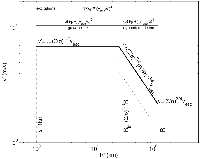
Figure 2: Schematic plot of the random-velocity spectrum in the collisionless case where all random velocities are in the dispersion-dominated regime. The spectrum comprises two power-law segments shown as bold solid lines. The rate at which viscous stirring by big bodies excites random velocities is given above the upper horizontal line. Rates that limit random velocities are written above the lower horizontal line and identified immediately below it. Each power-law segment of the spectrum is determined by equating the excitation rate to the relevant limiting rate. Radii bounding each segment are written along vertical dashed lines. Starting from the left, the first segment describes viscous stirring limited by the growth time of the big bodies, and the second viscous stirring is limited by dynamical friction. Parameters chosen for this figure are $t\sim 20{\,\rm Myr}$, $\sigma=0.2{\,\rm g}{\,\rm cm}^{-2}$, $\Sigma=\sigma/100$, $a=35{\,\rm AU}$, $\rho=1{\,\rm g}{\,\rm cm}^{-3}$, and $s=1{\,\rm km}$. For comparison, the dotted line shows the spectrum at $t=15{\,\rm Myr}$ with all other parameters held fixed.

Our approach captures some of the essential features found by detailed simulations. In Appendix B, we show how it can be extended to give the velocity spectrum when collisions are important. However, our approach is incomplete because we lack an evolution equation for $\Sigma$. This limitation is removed during the oligarchic stage of planet growth during which $\Sigma$ may be directly related to $R$ (Sections 9-10).

7.3.4 Collisional Solution

When collisions between small bodies are important, $u$ is damped by collisions at the same rate as it is excited by viscous stirring, i.e., Equation 60 vanishes, so

$${u\over v_{H}} \sim \alpha^{-2}{\Sigma\over\sigma}{s\over R}\ \ \ \ \ ,\ \ \ \ u<v_{H}$$ (75)

$${u\over v_{H}} \sim \left(\alpha^{-2}{\Sigma\over\sigma}{s\over R}\right)^{1/4}\ \ \ ,\ \ \ \ u>v_{H},$$ (76)

after using $v_{\rm esc}\sim v_{H}\alpha^{-1/2}$. For fixed $s$, $u$ grows to super-Hill values at late times as long as $\Sigma$ increases faster than $R$.

We select the case $v>v_{H}$ and, by implication, $u>v_{H}$, in which to solve Equation 59 for $(1/R)dR/dt\sim 1/t$. This case may be relevant at the end of planet formation.

From Section 7.3.2, big bodies grow by accreting small ones, and Equation 59 yields

$$t\sim\Omega^{-1}{\rho R\over\sigma}\left({\Sigma\over\sigma}{s\over R}\right)^{1/2}\ .$$ (77)

There are two restrictions on $R/s$ and $\Sigma/\sigma$:

$$v>v_{H} \Rightarrow {R\over s}<\alpha^{-2}\left({\Sigma\over\sigma}\right)^{2}$$ (78)

$$t>t_{\rm collide} \Rightarrow {R\over s}>{\sigma\over\Sigma}\ .$$ (79)

In this regime, it is always true that $u>u_{\rm esc}$ and $v<v_{\rm esc}$.

8 Orderly, Neutral, and Runaway Growth

The distribution function for the radii of large bodies can evolve in three qualitatively different ways: In orderly growth, the growth rate $(1/R^{\prime})dR^{\prime}/dt$ at a fixed time decreases with increasing $R^{\prime}$. Thus as big bodies grow, their radii converge, and the radius distribution function becomes progressively narrower. In runaway growth, $(1/R^{\prime})dR^{\prime}/dt$ increases with increasing $R^{\prime}$. Therefore the radius of the largest body increases fastest and runs away from the radii of all smaller bodies. The extreme high-$R^{\prime}$ end of the distribution develops a tail to infinity (Safronov 1972, Lee 2000, Malyshkin & Goodman 2001). In neutral growth, $(1/R^{\prime})dR^{\prime}/dt$ is independent of $R^{\prime}$. The radii of all bodies grow at the same rate, so the distribution function of relative radii does not evolve.

From Equation 41 with $v_{\rm esc}^{\prime}\propto R^{\prime}$,

$${1\over R^{\prime}}{dR^{\prime}\over dt}\propto\cases{R^{\prime-1}\Rightarrow{\rm orderly}&$u>v_{\rm esc}^{\prime}$\cr R^{\prime}\Rightarrow{\rm runaway}&$v^{\prime}_{\rm esc}>u>v^{\prime}_{H}$\cr 1\Rightarrow{\rm neutral}&$v_{H}^{\prime}>u>\alpha^{1/2}v_{H}^{\prime}$\cr R^{\prime-1}\Rightarrow{\rm orderly}&$\alpha^{1/2}v_{H}^{\prime}>u$},$$ (80)

where $u$ is the random velocity of the accreted bodies. Whether growth is in the orderly, neutral, or runaway regime is crucial for understanding how the mass spectrum evolves. However, it is less important for following the evolution in the two-groups approximation (see Section 7.2), where big bodies are defined as those that dominate the stirring and small bodies as those that dominate the mass density.

Runaway growth was discussed in Safronov (1972, ch. 9, p. 105). However, it is usually attributed to later works by Greenberg et al. (1978) and Wetherill & Stewart (1989), who found that the mass spectra in their particle-in-a-box simulations developed high-mass tails containing a small number of bodies. Wetherill & Stewart (1989, 1993) claimed that dynamical friction was essential for runaway growth; this view is now widely accepted, although it is misleading.

Runaway growth requires $v_{H}^{\prime}<u<v_{\rm esc}^{\prime}$. Dynamical friction, which reduces $v^{\prime}$ relative to $u$, does not affect these inequalities. Wetherill & Stewart’s conclusion was a consequence of the initial conditions they chose for their simulations. Initial velocities of all bodies were set comparable to the escape speed from the biggest body. But the biggest body was just outside of the runaway regime—its escape velocity was not sufficiently larger than its velocity relative to other bodies. By reducing the random velocity of the biggest body, dynamical friction tipped the balance in favor of runaway growth.

Adding the dependence on $u$ to Equation 80 in the runaway regime results in

$${1\over R^{\prime}}{dR^{\prime}\over dt}\propto{R^{\prime}\over u^{2}}\ \ \ ,\ v^{\prime}_{\rm esc}>u>v^{\prime}_{H}\ .$$ (81)

If $u$ does not evolve,

$$R^{\prime}(t)={R^{\prime}(0)\over 1-t/t_{\infty}}\ ,$$ (82)

for $t<t_{\infty}$, where $t_{\infty}$ depends on $R^{\prime}(0)$. However, the divergence of $R^{\prime}$ in finite time does not typify runaway growth. Typically, $u$ increases on the same timescale as $R$, the radius of the big bodies that viscously stir. For example, in the collisionless case, $u\propto\Sigma^{1/2}R$ (Equation 65), and for constant $\Sigma$, $u\propto R\propto t$ (see Equation 66). Inserting $u\propto t$ into Equation 81 shows that as $t\rightarrow\infty$ growth slows down, i.e., $(1/R^{\prime})dR^{\prime}/dt\propto 1/t^{2}$ decreases with increasing $t$. However, the evolution is still in the runaway regime because two big bodies of radii $R_{1}^{\prime}$ and $R_{2}^{\prime}$ grow at the relative rates

$${d\ln R_{1}^{\prime}/dt\over d\ln R_{2}^{\prime}/dt}={R_{1}^{\prime}\over R_{2}^{\prime}}\ ,$$ (83)

which implies that the radius of the larger body runs away from that of the smaller. Runaway addresses how the radii of two large bodies increase with respect to each other and not how each individually evolves in time. In the literature, these two distinct behaviors are frequently confused. For example, it is often stated that runaway ends when big bodies are more effective at viscous stirring than are small ones (e.g., IM93; Raf03c; Thommes, Duncan & Levison 2003). This leads to the condition $\Sigma M\sim\sigma m$ for when runaway ends. But the evolution can still be in the runaway regime while big bodies dominate the stirring. Although $\Sigma M\mathrel{\hbox{\hbox to0.0pt{\hbox{\lower 4.0pt\hbox{$\sim$}}\hss}\hbox{$>$}}}\sigma m$ is a necessary condidtion for oligarchy to occur (see below), it is not sufficient.

If runaway does not end when large bodies start stirring small ones, when does it end? There are at least three possibilities: (a) when the large bodies grow sufficiently such that the small bodies become sub-Hill (subsequent growth is neutral); (b) when the small bodies’ speed grows beyond the escape speed from big bodies (subsequent growth is orderly); (c) when oligarchy begins (discussed next).

9 Dispersion-Dominated Oligarchy, $u>v_{H}$

9.1 Transition from Runaway to Oligarchy

At late times, each big body is solely responsible for the viscous stirring of all bodies that cross its orbit; each big body heats its own food. The random velocities of small bodies that cross the orbit of a big body depend on the big body’s radius $R$; that is, $u=u(R)$. Provided $u(R)\propto R^{\gamma}$ with $\gamma>1/2$, the radii of big bodies converge (see Equation 81). Below, we show that $\gamma=6/5$, assuming that the size of the small bodies does not evolve (see Equation 100), although this is a questionable assumption. Consequently, growth changes from runaway to orderly. Kokubo & Ida (1998) coined the term oligarchy to describe this situation. Oligarchy may be the final stage of planet formation in the outer Solar System, although oligarchy with $u<v_{H}$ (see Section 10) may be the more relevant case. The final size of the oligarchs is insensitive to their earlier evolution.

9.2 How Oligarchy Proceeds: Battling Oligarchs

Each oligarch dominates an annulus of width $u/\Omega$ within which the small bodies cross its orbit. As the oligarchs increase $u$ by viscous stirring, two neighboring annuli—each with its own locally dominant big body—merge. Once the two big bodies enter the same feeding zone, they share small bodies, so the ratio of their growth rates is equal to the ratio of their radii. Then the radius of the larger body runs away from that of the smaller one. Even though oligarchs in separate annuli experience orderly growth, those that enter the same annulus experience runaway growth. This behavior continues on ever larger scales until nearly all the small bodies are consumed. Thus oligarchs maintain a separation of $\Delta a\sim u/\Omega$, and their surface density is

$$\Sigma \sim {M\over a\Delta a}\sim{\rho R^{2}\alpha\over a}{v_{H}\over u}\ ,\ \ \ u>v_{H}.$$ (84)

This equation fixes one of the free parameters discussed in Section 7. The chief remaining free parameter is the size of the small bodies.

Our description of oligarchy is in accord with that of Ida & Makino (1993). By contrast, Kokubo & Ida (1998) stated that, as the oligarchs grow, “orbital repulsion keeps their orbital separations wider than about 5 Hill radii.” They base this on N-body simulations containing a few oligarchs embedded in a sea of small bodies that dominate the surface density. Kokubo & Ida (1998) attributed the increasing orbital separation of the oligarchs to their mutual repulsion. However, this must result because their simulation took place within a narrow annulus. Orbital repulsion just depends on the surface density distribution and is independent of the sizes of the bodies. We do not expect neighboring oligarchs to move apart as they grow—there is no place for them to go. Clearly, the number of oligarchs must decrease with time. In the version of oligarchy by Kokubo & Ida (1998), neighboring oligarchs rule in harmony. In our version, oligarchs continually battle their neighbors for local dominance in a winner-takes-all war. So “battling oligarchs” might be a more appropriate term to describe this phase of planet formation. Indeed, competition between oligarchs has been observed in the numerical simulations of Kokubo & Ida (2000).

9.3 When Oligarchy Ends: Isolation Radius and Isolation Time

We refer to the epoch when nearly all the small bodies have been consumed as isolation. At isolation, $\Sigma$ and $R$, respectively, are given by $\Sigma_{\rm iso}\sim\sigma$ and (from Equation 84)

$$R_{\rm iso}\sim\left({\sigma\over\rho}{a\over\alpha}{u\over v_{H}}\right)^{1/2}\ .$$ (85)

This occurs on the timescale (Equation 41)

$$t_{\rm iso}\sim\Omega^{-1}\alpha{\rho\over\sigma}\left({u\over v_{H}}\right)^{2}R_{\rm iso}$$ (86)

We have yet to determine $u$ at isolation. Small-body velocities are likely damped by inelastic collisions. Otherwise, Uranus and Neptune would have taken far too long to form (see Section 6.4). Balancing viscous stirring by an oligarch with inelastic collisions as done in Equation 76, we find $u/v_{H}\sim\alpha^{-1/2}(s/R)^{1/4}$. Combining this with Equation 85, we can solve for

$${u\over v_{H}}\Big{|}_{\rm iso} \sim \alpha^{-1/3}a^{-1/9}\left({\sigma\over\rho}\right)^{-1/9}s^{2/9}\ ,$$ (87)

$$R_{\rm iso} \sim \alpha^{-2/3}a^{4/9}\left({\sigma\over\rho}\right)^{4/9}s^{1/9}\ .$$ (88)

The isolation time is then

$$t_{\rm iso} \sim \Omega^{-1}\alpha^{-1/3}a^{2/9}\left({\sigma\over\rho}\right)^{-7/9}s^{5/9}\ .$$ (89)

9.3.1 Numerical Expressions with $s=1$ km

In Appendix C (Section 15.2), we calculate the radius of the largest body that can condense out of a gravitationally unstable cold disk while conserving its internal angular momentum. In the minimum mass solar nebula, this critical radius is $s\sim 1{\,\rm km}$, independent of $a$. Motivated by this result, we set $s=1{\,\rm km}$ in the above formulae to obtain numerical expressions. Setting $\sigma=\sigma_{\rm MMSN}$ (Equation 53) then yields

$${u\over v_{H}}\Big{|}_{\rm iso} \sim 4\left({a\over 10\ {\rm AU}}\right)^{7/18}$$ (90)

$$R_{\rm iso} \sim 10,000\left({a\over 10\ {\rm AU}}\right)^{4/9}{\,\rm km}$$ (91)

$$t_{\rm iso} \sim 50\left({a\over 10\ {\rm AU}}\right)^{26/9}{\,\rm Myr}\ .$$ (92)

With $a\sim 30$ AU, oligarchic growth can produce $16,000$-km bodies in 1 Gyr out of the minimum mass solar nebula. Nonetheless, we regard this mode of growth as implausible. The small bodies’ random speed $u\sim$ km/s greatly exceeds their surface escape speed, $u_{\rm esc}\sim$ m/s. Collisions at these great speeds are almost certainly destructive. Hence $s$ is likely much smaller than 1 km. Collisional fragmentation has been considered by Inaba, Wetherill & Ikoma (2003), Kenyon & Bromley (2004) and Rafikov (2003e).

9.3.2 Varying $s$ at 30 AU

We can see how $R_{\rm iso}$ and $t_{\rm iso}$ vary with $s$ from Equations 88–89. But in deriving these equations, we made a number of assumptions that restrict their range of validity. First, we assumed $u>v_{H}$ at isolation, which implies $s>R\alpha^{2}$, i.e.,

$$s>30{\,\rm cm}\ .$$ (93)

at $a=30$ AU. Second, we assumed $u<\Omega a$; otherwise small bodies would be ejected. This implies

$$s<200{\,\rm km}\ .$$ (94)

We also made the following assumptions, which always hold at isolation at 30 AU as long as $30{\,\rm cm}<s<200{\,\rm km}$: (a) $u>u_{\rm esc}$, (b) $u<v_{\rm esc}$, (c) the disk of small bodies is gravitationally stable, and (d) the small-body disk is optically thin. However, $t_{\rm iso}\mathrel{\hbox{\hbox to0.0pt{\hbox{\lower 4.0pt\hbox{$\sim$}}\hss}\hbox{$<$}}}5$ Gyr sets the more stringent upper limit of

$$s<10{\,\rm km}\ .$$ (95)

Because of collisional fragmentation, the upper limits on $s$ are largely irrelevant. But if small bodies are ground down to sizes smaller than $\sim 30$ cm, then oligarchy with $u<v_{H}$ must be considered (see Section 10).

9.4 A Worked Example

We now return to the early stages of oligarchic growth and follow the subsequent evolution of $R$ and $u$. Here we fix $a=30$ AU, which gives $\Omega^{-1}\sim 30$ y and $\sigma\sim 0.2$ g cm^-2 for the MMSN (Equation 53) , we set $\Sigma$ to its oligarchic expression (Equation 84), and we set $s=1$ km in the early stages. At later stages, fragmentation reduces $s$.

9.4.1 Stage 1: Collisionless Oligarchy

The value of $R$ at which oligarchy starts depends on the runaway mass spectrum for which we lack a simple model. We consider the evolution after $R$ reaches 100 km, assuming that oligarchy has begun by then. At this stage, viscous stirring proceeds faster than collisional damping. Ignoring collisions, $u$ and $R$ both increase on the same timescale. From Equations 65 and 66,

$${u\over v_{H}} \sim \left({R\over 100\ {\rm km}}\right)^{2/3}\ ,$$ (96)

$$R \sim 200\left({t\over{\rm Myr}}\right)^{3/7}{\,\rm km}\ .$$ (97)

We chose $R>100$ km to avoid the sub-Hill equations here.

9.4.2 Transition from Collisionless to Collisional Evolution

As collisionless oligarchy proceeds, $u$ increases at an ever-decreasing rate: $(1/u)du/dt\propto 1/t$. By contrast, the collision rate is constant, so eventually collisional damping balances viscous stirring. This happens on the collision time (Equation 64):

$$t_{\rm transition}\sim t_{\rm collide}\sim 10\ {\rm Myr}\ ,$$ (98)

when $R$ has reached

$$R_{\rm transition}\sim 500{\rm\ km}\ .$$ (99)

At this time, $u_{\rm transition}\sim 10$ m/s, which exceeds the surface escape speed from kilometer-sized bodies, $u_{\rm esc}\sim 1$ m/s. Hence collisions might be destructive as soon as they commence. But it is also possible that intermolecular forces provide some cohesion to the small bodies and that the threshold speed for destruction is as high as 100 m/s. For definiteness, we assume that collisions are not destructive at the transition to collisional oligarchy, although this is highly uncertain.

9.4.3 Stage 2: Collisional Oligarchy

Equating the rates of viscous stirring and collisional damping (Equation 76) yields

$${u\over v_{H}}\sim 2\left({R\over 100\ {\rm km}}\right)^{1/5}\ .$$ (100)

and, from Equation 77,

$$R\sim 10,000\left({t\over{\rm Gyr}}\right)^{5/7}{\,\rm km}\ .$$ (101)

Collisional evolution continues until isolation ($\Sigma\sim\sigma$). If small bodies kept $s\sim$ 1 km, isolation would occur when $t\sim 1$ Gyr and $R\sim 10,000$ km. But by then, $u$ would be $\sim 1$ km/s. Collisions at these speeds would undoubtedly be destructive.

9.4.4 Stage 3: Collisional Oligarchy with Fragmented Bodies

At some stage before the oligarchs become planets, small bodies fragment, reducing $s$ far below 1 km. Smaller $s$ implies smaller $u$ and, hence, faster accretion: If we reintroduce the dependence of Equation 101 on $s$ and solve for $t$, we find $t\sim(R/10,000{\,\rm km})^{7/5}(s/{\,\rm km})^{2/5}$ Gyr. If $s\sim 30$ cm, planet-sized bodies form in 100 Myr. In fact, it is possible that $s\ll 30$ cm, in which case the planets form even faster. But then, $u<v_{H}$ at isolation (Equation 93). This leads us to examine oligarchy in the shear-dominated limit.

10 Shear-Dominated Oligarchy: $u<v_{H}$

Oligarchy with $u<v_{H}$ is not well treated in the literature. It differs qualitatively from oligarchy with $u>v_{H}$ in several respects:

• As time progresses, oligarchs that previously were isolated begin to compete with their neighbors to accrete the same small bodies. For $u<v_{H}$, growth is in the neutral regime, and the ratio of the radii of big bodies maintains a constant value. By contrast, for $u>v_{H}$, growth is in the runaway regime, and the ratio of radii diverges.

• For $u<v_{H}$, an oligarch accretes from an annulus of width $\sim R_{H}$ and stirs a wider annulus of width $\sim(v_{H}/u)^{1/2}R_{H}$. By contrast, for $u>v_{H}$, an oligarch both excites and accretes small bodies from an annulus of width $\sim u\Omega^{-1}$.

• For $u<v_{H}$, the oligarchs lie in a flat disk and may accrete each other efficiently.

Each of these items raises a question about oligarchy in the shear dominated regime:

• Can shear-dominated oligarchy be maintained as oligarchs grow?

• Is the spacing between oligarchs set by their feeding zones or by their excitation zones?

• Do oligarchs grow more by coalescing than by eating small bodies?

In the shear-dominated limit, we show that oligarchy, defined as a single big body in its feeding zone of width $\sim R_{H}$, is usually maintained, particularly at late times. As each big body accretes small bodies, its feeding zone expands. Once neighboring oligarchs enter each other’s feeding zones, they quickly coalesce. We can see this as follows: Oligarchs coalesce at the rate $\alpha^{-3/2}\Sigma\Omega/\rho R$, and they grow by accreting small bodies at the rate $\alpha^{-1}(v_{H}/u)\sigma\Omega/\rho R$. When neighboring oligarchs enter each others’ feeding zones, growth by coalescence is faster than that by accretion of small bodies, provided

$${\Sigma\over\sigma}\alpha^{-1/2}{u\over v_{H}}>1\ ,$$ (102)

which holds for $\Sigma$ not much smaller than $\sigma$. This ensures that there is typically only one big body within each feeding zone and justifies our definition. Growth proceeds in two phases: Oligarchs slowly grow by accreting small bodies. Upon doubling their mass, they enter their neighbors’ feeding zones. Rapid coalescence follows. On average, growth by coalescence is comparable to that by accretion of small bodies.

When $u<v_{H}$, an oligarch stirs a region of size $(v_{H}/u)^{1/2}R_{H}$, which is larger than its feeding zone. Within that stirring region, oligarchs keep their original size ratio. Outside that region, there is an effect similar to that in dispersion-dominated oligarchy, where oligarchs grow to similar sizes because each oligarch regulates its own growth by heating its own food. If stirring in one heating zone is large, growth in that zone slows down. Thus oligarchs within each heating zone collectively regulate their own growth, and $\Sigma$ tends to become uniform on scales larger than the stirring scale $(v_{H}/u)^{1/2}R_{H}$.

Because the oligarchs’ separation is $\Delta a\sim R_{H}$, their surface density is

$$\Sigma\sim{M\over a\Delta a}\sim{\rho R^{2}\alpha\over a}\ \ ,\ \ u<v_{H}\ \ .$$ (103)

This is the standard expression used in the literature, but it has been incorrectly applied to the case $u>v_{H}$ (KI98; Thommes, Duncan & Levison 2003). At the end of sub-Hill oligarchy, when $\Sigma\sim\sigma$, the final value of the oligarchs’ radii is given by equating the above expression with $\sigma$, which gives the isolation radius

$$R_{\rm iso}\sim\left({\sigma a\over\rho\alpha}\right)^{1/2} \sim 12,000\left(a\over 10{\rm\ AU}\right)^{1/4}{\,\rm km}\ .$$ (104)

In the numerical expression, we have included factors of order unity (Equation 58). At isolation, $u<v_{H}$ only if $s<200(a/{\rm 10\ AU})^{-7/4}{\,\rm cm}$. Larger values of $s$ are compatible with $u<v_{H}$ at earlier stages of planet growth.

10.1 The Fastest Oligarchy

The fastest possible accretion rate is faster than the geometrical rate by $\alpha^{-3/2}$, and occurs for $u\sim\alpha^{1/2}v_{H}$. Therefore

$$t_{\rm fastest}\sim\alpha^{3/2}{\rho R\over\sigma\Omega}\sim 30,000\left({a\over{\ 10\rm AU}}\right)^{7/4}{\,\rm y}.$$ (105)

More precisely, this is the shortest time during which an oligarch could double in mass. Oligarchy can proceed so fast that more time might be spent in forming kilometer-sized small bodies than in growing these bodies into planets.

Gravitational stability of the disk (see Section 15.2) dictates a minimum velocity dispersion of

$$u_{\rm min}\sim{\sigma\Omega\over\alpha^{3}\rho}\sim 1{\rm m/s}.$$ (106)

With our nominal parameters, this is approximately equal to $\alpha^{1/2}v_{H}$ for bodies with the isolation radius (Equation 104). It is not clear whether the short timescale of Equation 105 can materialize. If $u\sim u_{\min}>\alpha^{1/2}v_{H}$, the oligarchs grow at a constant rate (i.e. exponentially) on the timescale

$$t_{\rm fastest,\ stability\ limited}\sim\alpha^{-1}\Omega^{-1}\sim 10,000\left(a\over 10{\,\rm AU}\right)^{2}{\,\rm y}.$$ (107)

To keep $u\sim u_{\rm min}$ with collisions, $s$ must be

$$s\sim{\sigma\over\rho}\sim\left({a\over 10{\ \rm AU}}\right)^{-3/2}{\,\rm cm}$$ (108)

when $\Sigma\sim\sigma$.

Rafikov (2003e) showed that accretion is very fast if the accreted bodies are very small and their random velocities are damped by gas drag. Lissauer’s (1987) expression for the fastest growth rate differs from ours. He assumed that the lowest $u$ possible is $v_{H}$ and, hence, that the fastest focusing factor is $\alpha^{-1}$. He argued that in a cold disk every encounter with a large body results in a velocity of $v_{H}$, so $u\mathrel{\hbox{\hbox to0.0pt{\hbox{\lower 4.0pt\hbox{$\sim$}}\hss}\hbox{$>$}}}v_{H}$. But this is incorrect because collisional damping between encounters can maintain $u<v_{H}$.

11 Beyond Oligarchy

Relatively little attention has been paid to stages of planet formation beyond oligarchy. Chambers (2001) reported results from an N-body simulation initialized with several-dozen bodies separated by a few times their Hill radii on coplanar, circular orbits. This setup is unstable; eccentricities and inclinations quickly develop. This raises two important questions: When in the course of oligarchic growth does this instability occur? And what is its outcome? These questions and others are addressed by Goldreich, Lithwick & Sari (2004), which the discussion here closely follows. We start by showing that oligarchy ends, and instability kicks in, when $\Sigma\approx\sigma$. This result applies to accretion in both shear- and dispersion-dominated regimes.

11.1 Before Oligarchy Ends: $\Sigma<\sigma$

When $\Sigma<\sigma$, the oligarchs’ velocity is set by a balance between mutual viscous stirring and dynamical friction with small bodies. If $u>v_{H}$, this results in

$$v\sim u\left({\Sigma\over\sigma}\right)^{1/4}\ \ ,\ \ u>v_{H}$$ (109)

(see Equation 63). If $u<v_{H}$, then, as we shall see below, $v<v_{H}$ as well. So viscous stirring excites $v$ at the rate $\alpha^{-2}(\Sigma\Omega/\rho R)v_{H}/v$ (Equation 44), and dynamical friction damps it at the rate $\alpha^{-2}\sigma\Omega/\rho R$ (Section 5.5). Equating stirring and damping yields

$$v\sim v_{H}{\Sigma\over\sigma}\,\ \ ,\ \ u<v_{H}\ \ .$$ (110)

This justifies the use of rates appropriate to $v<v_{H}$.

11.2 Instability Of Protoplanet’s Velocity Dispersion: $\Sigma>\sigma$

As soon as $\Sigma>\sigma$, the velocity dispersion of the big bodies destabilizes. This occurs because the typical relative velocity between a big and small body is $v>u$, so the velocity evolution equation becomes (see Section 5.5):

$${1\over v}{dv\over dt}={\left(\Sigma-\sigma\right)\Omega\over\rho R}\alpha^{-2}\left({v_{H}\over v}\right)^{4},$$ (111)

regardless of whether $u<v_{H}$ or $u>v_{H}$. Thus when $\Sigma>\sigma$, big bodies are heated faster than they are cooled. This marks the end of oligarchy. As $v$ increases, heating and cooling both slow down, but heating always dominates cooling. Rather quickly, the orbits of neighboring big bodies cross.

Because it is based on approximate rates for viscous stirring and dynamical friction, the criterion, $\Sigma\sim\sigma$, for the onset of velocity instability is also approximate. N-body simulations of oligarchy with the addition of accurate analytic expressions for dynamical friction are needed to identify the critical surface density ratio.

The consequence of the instability in the velocity dispersion differs according to which is larger, the escape velocity from the surfaces of the planets that ultimately form or the escape velocity from their orbits. The ratio of these two escape velocities, $v_{\rm esc}/\Omega a$, is

$${\cal R}\sim\cases{0.3&for $a=1{\,\rm AU}\,\,\&\,\,M_{p}=M_{\oplus}$\cr 2.3&for $a=25{\,\rm AU}\,\,\&\,\,M_{p}=15M_{\oplus}$}\,,$$ (112)

where $M_{p}$ is the mass of a planet and $M_{\oplus}$ is Earth’s mass.

11.2.1 Inner Solar System, ${\cal R}\ll 1$: Coalescence

In regions where ${\cal R}\ll 1$, the big bodies’ velocity dispersion increases until it becomes comparable to the escape velocity from their surfaces. At this point, they begin to collide and coalesce. Coalescence slows as the number of big bodies decreases and their individual masses increase.

The timescale for the formation of planet-sized bodies with radius $R_{\rm p}$ whose orbits are separated by $\sim a$ is

$$t_{\rm coag}\sim\left(\rho R_{p}\over\sigma\Omega\right)\sim 10^{8}{\,\rm y}\,\,{\rm at\,\,}a=1{\,\rm AU}\,\,{\rm for}\,\,R_{p}=R_{\oplus}\,.$$ (113)

At a separation of order $a$, mutual interactions no longer produce chaotic perturbations. Indeed, the N-body simulations of Chambers (2001) produce stable systems on a timescale similar to $t_{\rm coag}$.

What happens to the small bodies while the big ones are colliding and coalescing? On one hand, a significant fraction collide with and are accreted by big bodies. On the other hand, new small bodies are created in grazing collisions between big ones, ensuring that a significant residual population of small bodies persists until the end of coalescence.

11.2.2 Outer Solar System, ${\cal R}\gg 1$: Ejection

In regions where ${\cal R}\gg 1$, $v$ reaches the orbital speed $\Omega a$. Some fraction of the big bodies becomes detached from the planetary system and either takes up residence in the Oort cloud or escapes from the Sun. This continues until mutual interactions among the surviving big bodies are no longer capable of driving large-scale chaos.

We estimate the ejection timescale as

$$t_{\rm eject}\sim{0.1\over\Omega}\left(M_{\odot}\over M_{p}\right)^{2}\sim 10^{9}{{\,\rm y}}\,\,{\rm at\,\,}a=25{\,\rm AU}\,.$$ (114)

Shoemaker & Wolfe (1984) and Dones et al. (2004) reported similar timescales for the ejection of test particles placed on orbits between Uranus and Neptune, the former authors from a crude impulsive treatment of scattering and the latter authors from N-body integrations. A shorter timescale might apply if bodies were transferred to and then ejected by Jupiter and Saturn.

As the random velocity of a big body increases, the rate at which it accretes small bodies declines. Thus a substantial surface density of small bodies is likely to remain after most the big bodies have been ejected.

11.3 Orbit Regularization

Either coagulation or ejection is likely to end with the surviving big bodies moving on orbits with eccentricities and inclinations of order ${\cal R}\sim 0.3$ in the inner-planet system and of order unity in the outer-planet system. Chambers (2001) saw the former in N-body simulations. Such orbits do not resemble those of planets in the Solar System. In reality, dynamical friction by the residual small bodies tends to circularize and flatten the orbits of the surviving protoplanets.

As the surviving planets cool down, their orbits no longer cross. Gaps may open in the disk of small bodies around the planets’ orbits. Dynamical friction continues to act after gap opening. Angular momentum and energy are transferred between the planet and the disk of small particles by torques that the planet exerts at Lindblad and corotation resonances. Ward & Hahn (1998, 2003) used the standard torque formula (Goldreich & Tremaine 1980) and concluded that the most potent contributions to the damping of eccentricity and inclination are due to torques at apsidal and nodal resonances. The analysis of Goldreich & Sari (2003), when applied to the cold planetesimal disks, suggests that the apsidal torque will be the most potent one, albeit with lower magnitude than Ward & Hahn (1998, 2003) had calculated.

11.4 Clean Up

What was the fate of the residual small bodies that remained after the protoplanets had settled onto stable orbits? Velocity instability started when small bodies and protoplanets contributed comparably to the overall surface density. But today, the mass in small bodies is much less than that in planets. Clean up was both the last and longest stage in the evolution of the Solar System. It is ongoing in both the asteroid and Kuiper belts. The Oort comet cloud was probably populated during this stage. Some thoughts on how clean up was achieved are sketched in Goldreich, Lithwick & Sari (2004).

12 Summary

We begin this review (Sections 2–5) with an overview of the physics of coagulation: how bodies in a circumsolar disk grow by accreting each other, and how they stir and damp each other’s velocities through viscous stirring and dynamical friction. We present order-of-magnitude derivations for relevant formulae that capture the underlying physics. For $u<v_{H}$, a small fraction of the bodies contains a large fraction of the energy in random motions, and inclinations are stirred less than eccentricities, which can lead to a very flat disk. In this limit, viscous stirring has not been correctly treated in the literature.

In Sections 6–10, we focus on the growth of Uranus and Neptune, whose masses and formation times greatly constrain how they formed. Because these planets do not contain a lot of gas, we neglect gas drag. But in Appendix A, we show that gas drag can simply be accounted for by setting the effective size of small bodies below its true value.

A simple argument (see Section 6) shows that Uranus and Neptune grew by accreting bodies that were smaller than 1 km. Had the accreted bodies been bigger than 1 km, they would not have collided with each other sufficiently frequently to damp their speeds, which are vigorously stirred by the planetary embryos. Accretion of such hot bodies would have taken longer than the age of the Solar System.

In Section 7, we consider accretion more quantitatively. The two-groups approximation is a valuable tool. Often, only two groups of bodies—those with most of the mass and those that dominate viscous stirring—control the evolution of all others. It is nearly trivial to write down the equations describing the evolution of the two groups and not difficult to solve them. Because the rest of the bodies behave passively, their velocity spectrum is also easy to work out (see Appendix B). The two-groups approximation is helpful in analyzing results from N-body simulations and particle-in-a-box simulations. However, we have been unable to arrive at a simple quantitative picture for how the mass spectrum evolves. Simulations are still needed for that. In Section 8, we address qualitatively the different ways in which the mass spectrum can evolve, by orderly, neutral, or runaway growth.

In Sections 9–10, we discuss oligarchy with $u>v_{H}$ and with $u<v_{H}$. Dispersion-dominated oligarchy begins when each big body heats its own food, i.e., when the large bodies’ orbits are separated by $u/\Omega$. Because oligarchs regulate their own growth, their masses equalize. We derive expressions for the final sizes of the oligarchs as well as their formation times. The formation time is quite sensitive to the assumed value of the small bodies’ radii. Shear-dominated oligarchy begins when the large bodies’ orbits are separated by a few times their Hill sphere. Discussions of oligarchy in the literature mix elements from dispersion-dominated and shear-dominated oligarchy. We show that oligarchy pertains in both regimes, albeit with different behaviors. Oligarchy does not occur for very flat disks with $u<\alpha^{1/2}v_{H}$.

We outline two scenarios for the formation of Uranus and Neptune. If the accreted bodies were $\sim$1 km, then Uranus and Neptune would have formed in a few billion years (Equations 57, 91, and 92). Kilometer-sized bodies are a natural outcome of gravitational instability of a planetesimal disk (see Appendix C). However, we do not view the solution with kilometer-sized bodies as physical. Uranus and Neptune would excite the velocity dispersion of these bodies to such an extent that they would shatter when they collided, thereby creating much smaller bodies. This leads us to favor a scenario in which the accreted bodies were much smaller than 1 km. In the limit in which collisions reduced the radii of the accreted bodies to a few centimeters or less, the final doubling of the masses of Uranus and Neptune could have taken less than one million years (Equations 105, 107, and 108) . Although this resolves the timescale problem, it comes with its own caveat. In the minimum mass solar nebula, shear-dominated accretion leads to the formation of 10 small planets beyond Saturn (Equations 58 and 104). Why, then, are we left with 2 large ones? We suggest that Uranus and Neptune have collected most of their mass by the end of oligarchy. This requires an initial surface density of a few times that of the MMSN. The uncertainties are (a) the exact epoch when oligarchy ends and velocity instability begins, (b) the radial range from which oligarchs can accrete, and (c) the amount of mass that surviving planets can accrete during the cleanup stage. Other planet-sized objects probably formed in and were ejected from the outer Solar System after oligarchy.

We conclude with a discussion of post-oligarchic stages. Velocity instability leads to ejection of bodies from the outer-planet system and to their coagulation in the inner one. It ceases once the number of protoplanets is sufficiently reduced. After that, dynamical friction from the residual small bodies damps the protoplanets’ orbital eccentricities and inclinations. The last and longest stage is also the least understood one: cleanup of the remaining small bodies. Wide gaps that form around the orbits of the surviving planets inhibit accretion. Collisions prevent the outer planets from ejecting small bodies from the outer-planet region. Very little attention has been paid to cleanup. It is a frontier in planet formation worth exploring.

13 Appendix A: Neglected Effects

13.1 Gas Drag

One of the main effects of gas drag is to damp the random velocities of small bodies. This is simply accounted for in our formalism. Damping by inelastic collisions is inversely proportional to $s$, and $s$ appears only in connection with damping by inelastic collisions. To account for gas drag, it suffices to set $s$ to a value smaller than the true size of the small bodies. As we have emphasized, the size of the small bodies is highly uncertain. In the following, we estimate the gas-damping rate (for more complete treatments, see Adachi, Hayashi & Nakazawa 1976, Rafikov 2003e).

Gas drag damps a small body’s random velocity in the time that the body encounters a mass of gas equal to its own mass. Thus

$${{\rm gas\ damping\ rate}\over{\rm collisional\ damping\ rate}}\sim{\rho_{\rm gas}\over\rho_{\rm bodies}}{\Delta u_{\rm gas}\over u}\sim{\sigma_{\rm gas}\over\sigma}{\Delta u_{\rm gas}\over c_{s}}\ ,$$ (115)

where $\rho_{\rm gas}$ and $\rho_{\rm bodies}$ are the midplane mass densities of the gas and the small bodies, $\sigma_{\rm gas}$ and $c_{s}$ are the surface density and sound speed of the gas, and $\Delta u_{\rm gas}$ is the speed at which a small body encounters the gas. We assume that $u<c_{s}$, so the scale height of the gas disk is larger than that of the small bodies. In fact, we assume below the slightly more restrictive condition $u<c_{s}^{2}/\Omega a$, which almost certainly holds within the first 10 Myr in the outer Solar System.

We have yet to calculate $\Delta u_{\rm gas}$. There are two limiting regimes, depending on the size of the small body relative to the mean free path of a gas molecule $l_{\rm mfp}$. When $s<l_{\rm mfp}$, gas particles act as tiny bodies whose random speed is $c_{s}$ (i.e., the free molecular drag, or Epstein, regime), so $\Delta u_{\rm gas}\sim c_{s}$ and Equation 115 becomes

$${{\rm gas\ damping\ rate}\over{\rm collisional\ damping\ rate}}\sim{\sigma_{\rm gas}\over\sigma}\ \ ,\ \ \ \ s<l_{\rm mfp}\ .$$ (116)

For sufficiently large $s$, the gas can be treated as a collisional fluid, and $\Delta u_{\rm gas}$ is the speed at which a small body moves through the gas (the turbulent drag regime). There is an intermediate regime in which Stokes (viscous) drag applies. We ignore this and consider the limiting case of turbulent drag. Small bodies move relative to the gas because the orbital speed of the gas around the Sun is sub-Keplerian owing to thermal pressure support, i.e., $V_{\rm gas}^{2}\sim(\Omega a)^{2}-c_{s}^{2}$, where $V_{\rm gas}$ is the gas’s orbital speed. Thus $\Delta u_{\rm gas}\sim\Omega a-V_{\rm gas}\sim c_{s}^{2}/(\Omega a)$, to lowest order in $c_{s}/(\Omega a)$. Equation 115 becomes

$${{\rm gas\ damping\ rate}\over{\rm collisional\ damping\ rate}}\sim{\sigma_{\rm gas}\over\sigma}{c_{s}\over\Omega a}\ \ ,\ \ \ \ s>{\Omega a\over c_{s}}l_{\rm mfp}\ ,$$ (117)

where the limit on $s$ ensures that the Reynolds number exceeds unity.

Numerically,

$${\sigma_{\rm gas}\over\sigma}\sim 100\ ,$$ (118)

for cosmic composition and condensates expected in the outer Solar System. We approximate the gas temperature by equating it to the local equilibrium temperature, $T_{\rm gas}\sim T_{\odot}\alpha^{1/2}$, where $T_{\odot}\sim 6,000\,$K is the surface temperature of the Sun (for more-realistic models, see Chiang & Goldreich 1997). This yields $c_{s}\sim(k_{B}T_{\rm gas}/m_{p})^{1/2}\sim 6\alpha^{1/4}{\,\rm km}{\,\rm s}^{-1}$, where $k_{B}$ is Boltzmann’s constant and $m_{p}$ is the proton mass. Hence

$${c_{s}\over\Omega a}\sim 0.1\left({a\over 10\ {\rm AU}}\right)^{1/4}\ ,$$ (119)

and

$$l_{\rm mfp}\sim{m_{p}\over\rho_{\rm gas}\sigma_{\rm x-section}}\sim 300\ \left({a\over 10{\rm\ AU}}\right)^{11/4}\ {\,\rm cm},$$ (120)

where $\sigma_{\rm x-section}\sim 10^{-15}{\,\rm cm}^{2}$ is the collisional cross section of gas particles. Equation 116 shows that gas drag might damp the random velocities of small bodies as much as two orders of magnitude faster than inelastic collisions. Although the enhancement factors are not very sensitive to $a$, the sizes of the bodies at which transitions between drag regimes occur are extremely sensitive. Gas drag might also be important for the orbital decay of planetesimals (Adachi, Hayashi & Nakazawa 1976; Weiden77b). In addition, if a protoplanet has a gaseous atmosphere, then gas drag on planetesimals that pass through its atmosphere can enhance the accretion rate (Inaba & Ikoma 2003).

A potentially more significant effect of gas drag is its role in damping the random velocities of oligarchs. The velocities of large bodies can be damped by gas in the same way that it is damped by small bodies. Ward (1993) showed that the rate of gas damping can be obtained from the damping rate due to small bodies by substituting the surface density of gas for that of the small bodies and the sound speed of the gas, $c_{s}$, for the random velocity of the small bodies, $u$. The dispersion-dominated region is relevant because at isolation $v_{H}<c_{s}<v_{\rm esc}$. Moreover, we assume that $v<c_{s}$. By damping the oligarchs’ random velocities, gas drag could delay the onset of velocity instability and enable the oligarchs to consume all the small bodies.

In the inner Solar System, it is possible—although highly uncertain—that much of the gas survived until isolation. Then the full velocity instability of the oligarchs would have been delayed until the surface density of the gas declined to match that contributed by the oligarchs. After that, the oligarchs would have excited their random velocities up to their escape speeds. Although most the small bodies would have been accreted before this happened, plenty of new ones created in glancing collisions could have damped the orbital eccentricities and inclinations of the planets that finally formed. Gas is unlikely to have survived long enough to contribute to the regularization of their orbits.

Uranus and Neptune are believed to have collected only a few Earth masses of nebular gas. So it is likely that most the gas had disappeared prior to isolation in the outer Solar System.

13.2 Accretion of Gas

How did the giant planets accrete their gas? In the core accretion model, the cores of the gas giants first formed via coagulation. Once the cores were sufficiently massive, they gravitationally captured gas from the surrounding disk (Mizuno, Nakazawa & Hayashi 1978; Pollack et al. 1996).

Other formation mechanisms have been proposed. Most notable is gravitational instability of a gas disk, without the prior formation of a core. A sufficiently cold gas disk is gravitationally unstable and can collapse directly into giant gaseous planets (Boss 1997, Mayer et al. 2002). Jupiter and Saturn could have formed in this way, but only if the surface density was greater than the MMSN value by more than a factor of 10 Guillot & Gladman (2000). Some extra-solar planets might also have formed in this manner. Uranus and Neptune have only 10–20% gas, so it is likely that they formed via coagulation.

13.3 Other Neglected Effects

Jupiter and Saturn probably formed before Uranus and Neptune. Therefore they viscously stirred the planetesimals that were accreted onto Uranus and Neptune (KW00; Kuchner, Brown & Holman 2002). We neglect this because, in the late stages of accretion, stirring by the embryos of Uranus and Neptune is more important. We do not consider gap formation by a growing embryo Ward (1997); Rafikov (2001), although gaps might hinder growth. We also neglect the effects of solar radiation, such as radiation pressure, Poynting-Robertson drag, and the Yarkovsky effect (Burns, Lamy & Soter 1979).

14 Appendix B: Velocity Spectrum

We apply the two-groups approximation to determine the run of the typical random velocity with radius $R^{\prime}$, where $s<R^{\prime}<R$. Intermediate-sized bodies behave passively. They merely respond to viscous stirring by big bodies and dynamical friction by small ones. This is similar to our discussion in Section 7.3.3, except that here we consider big bodies with $v<v_{H}$ and small bodies that are collisional but maintain $u>v_{H}$. This introduces two additional transitions: one between collisional and collisionless behavior at $R_{col}$ and another at $R_{v_{H}}$, where $v^{\prime}=v_{H}$. We find

$$R_{col}=\left(\Sigma\over\sigma\right)^{1/2}\left(s\over R\right)^{1/2}R\,,$$ (121)

$$R_{fr}=\left(\Sigma\over\sigma\right)^{1/3}R\,,$$ (122)

$$R_{v_{H}}=\left(\Sigma\over\sigma\right)^{2/3}\left(s\over R\right)^{1/3}\alpha^{-2/3}R\,.$$ (123)

Figure 3 displays the entire random velocity spectrum for a specific choice of parameters: $\sigma=0.2{\,\rm g}{\,\rm cm}^{-2}$, $\Sigma=0.003\sigma$, $a=30{\,\rm AU}$, $s=1{\,\rm km}$, and $R=5000{\,\rm km}$. The choice of $R$ determines the time.

As discussed in Section 4.3 , the typical random velocity is similar to the velocity dispersion except for $v^{\prime}<v_{H}$. In the sub-Hill regime, $R_{v_{H}}<R^{\prime}<R$, the typical random velocity, $v^{\prime}/v_{H}\sim(R^{\prime}/R_{v_{H}})^{-3}$, is smaller than the rms velocity $v^{\prime}_{\rm rms}/v_{H}\sim(R^{\prime}/R_{v_{H}})^{-3/2}$. The latter implies energy equipartition among bodies in the sub-Hill regime as found in some simulations. This equipartition has a nonstandard origin. It results from a balance between viscous stirring by large bodies and dynamical friction from small ones, where the random energy of a big body is much larger than that of a small one (see Rafikov 2003d). In the sub-Hill regime (see Section 4.3), the distribution function of random velocities at fixed $R^{\prime}$ between the typical velocity and $v_{H}$ is a power law.

The spectral shape of the solution displayed in Figure 3 requires $s<R_{col}<R_{fr}<R_{v_{H}}<R$, supplemented by $u>v_{H}$. It also assumes that big bodies grow by accreting small ones, which holds if

$$\left(v_{H}\over u\right)^{2}>{\Sigma\over\sigma}\alpha^{-1/2}\,.$$ (124)

Equation 124 is marginally satisfied for the parameter values chosen in Figure 3. Other consistency constraints are that big bodies dominate the stirring and that small ones provide the dynamical friction. It is not difficult to choose size distributions that satisfy these constraints.

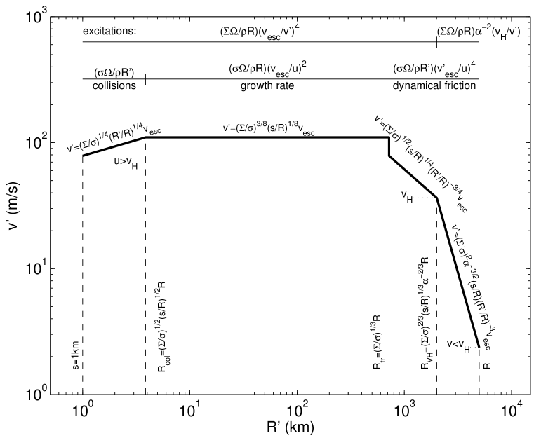
Figure 3: Schematic plot of the random velocity spectrum, including collisions. Small bodies are in the dispersion-dominated regime, and large ones are in the shear-dominated regime. The spectrum comprises four power-law segments (bold solid lines). Rates at which viscous stirring by big bodies excites random velocities are given above the upper horizontal line. Rates that limit random velocities are written above the lower horizontal line and identified immediately below it. Each power-law segement of the spectrum is determined by equating the excitation rate to the relevant limiting rate. Radii bounding each segment are written along vertical dashed lines. Dotted, horizontal line segments mark the values of the random velocities of the small bodies, $u$, the random velocities of the large bodies, $v$, and the Hill velocity of the large bodies, $v_{H}$. Starting from the left, the first, second, and third segments show viscous stirring in the dispersion-dominated regime limited by collisions, the growth time of big bodies, and dynamical friction, respectively. The fourth segment shows viscous stirring in the shear-dominated regime limited by dynamical friction. Here we are plotting the typical random velocity, which is smaller than the rms random velocity (described in Section 4.3). The discontinuity between the second and third segments is closely related to the velocity instability that occurs for $v>u$ (see Section 11.2). Parameters chosen for this figure are $R\sim 5,000{\,\rm km}$, $\sigma=0.2{\,\rm g}{\,\rm cm}^{-2}$, $\Sigma=0.003\sigma$, $a=30{\,\rm AU}$, $\rho=1{\,\rm g}{\,\rm cm}^{-3}$, and $s=1{\,\rm km}$.

15 Appendix C: Considerations Relevant to the Size of Small Bodies

Without a compelling reason to favor any particular radius for the small bodies, we have been treating $s$ as a free parameter. A smaller $s$ enhances the damping of $u$ by collisions and gas drag, which speeds up accretion. We suggest that as the big bodies grow, the small bodies undergo destructive collisions, which results in a fragmentation cascade. However, there is a floor on $u$ below which gravitational instabilities would lead to the rapid formation kilometer-sized bodies.

15.1 Destructive Collisions

Fragmentation has been considered by, e.g., Inaba, Wetherill & Ikoma (2003), Kenyon & Bromley (2004), and Rafikov (2003e). Even in the shear-dominated limit, $u<v_{H}$, a small body that passes within $R_{H}$ of a big body has its random velocity excited to order $v_{H}$, where

$$v_{H}\sim\Omega R_{H}\sim 10^{2}\left(R\over 10^{2}{\,\rm km}\right)\left(a\over 10{\,\rm AU}\right)^{-1/2}{\,\rm cm}{\,\rm s}^{-1}\,.$$ (125)

By comparison, the escape speed from the surface of a small body is

$$u_{\rm esc}\sim(G\rho)^{1/2}s\sim 10^{2}\left({s\over{\rm km}}\right){\,\rm cm}{\,\rm s}^{-1}\,.$$ (126)

This comparison reveals that the random velocity induced by large protoplanets may suffice to break up kilometer-sized planetesimals. At what stage this might happen depends on two unknowns: the size of planetesimals at the start of runaway growth and their internal strength Dohnanyi (1969).

Suppose that at some stage the initial planetesimals begin to fragment. As $s$ decreases, the collision rate $\sigma\Omega/(\rho s)$ (Equation 50) increases, which leads to an accelerating collisional cascade. Although collisions damp $u$, the planetary embryo viscously stirs it. Assuming that $u$ is set by a balance between collisional damping and viscous stirring, $u/u_{\rm esc}$ increases as $s$ decreases. Thus the collisions remain destructive so long as the stresses they induce exceed the yield stress of the material (ice) composing the small bodies. Whether this occurs before $u\sim u_{\rm min}$ (see Section 15.2) is unknown.

15.2 Gravitational Instability in a Cold Keplerian Particle Disk

In a disk of particles that orbit the Sun, if the particles’ velocity dispersion $u$ falls below the critical value

$$u_{\rm min}\sim{G\sigma\over\Omega}\sim 1{\,\rm m}/{\,\rm s}\ ,$$ (127)

then the disk is gravitationally unstable Binney & Tremaine (1987). For the minimum mass solar nebula (Equation 53), which we used in the above numerical expression, $u_{\rm min}$ is independent of $a$.

We consider the evolution of a cold disk with $u=0$. This disk is unstable. Overdense perturbations of size

$$l\mathrel{\hbox{\hbox to0.0pt{\hbox{\lower 4.0pt\hbox{$\sim$}}\hss}\hbox{$<$}}}l_{\rm crit}\sim{G\sigma\over\Omega^{2}}\sim\alpha^{-3}{\sigma\over\rho}\$$ (128)

collapse and virialize on the timescale

$$t_{\rm collapse}\sim\left({l\over G\sigma}\right)^{1/2}\ .$$ (129)

Perturbations with $l>l_{\rm crit}$ are stabilized by Keplerian shear or, equivalently, by the Sun’s tidal gravity.

Gravitational instabilities convert potential energy into kinetic energy of random motions. The development of nonlinear overdensities requires that this energy dissipate at the collapse rate. Otherwise the random velocity dispersion would be maintained near the margin of stability (Gammie 2001); i.e., $u\sim u_{\rm min}$. Inelastic collisions are the only option for dissipating energy in a particle disk. For the collision rate to match the collapse rate, the particle disk would have to be optically thick , $\sigma/\rho s\mathrel{\hbox{\hbox to0.0pt{\hbox{\lower 4.0pt\hbox{$\sim$}}\hss}\hbox{$>$}}}1$. An optically thick particle disk might result from a collisional fragmentation cascade.

Only those clusters that originate from patches of size $l_{*}$, where $l_{*}\ll l_{\rm crit}$, can contract to form solid bodies without getting rid of internal angular momentum. Here the asterisk subscript denotes quantities pertaining to the largest solid body that can form without angular momentum loss. Its angular momentum per unit mass, $(G\rho)^{1/2}s_{*}^{2}$, must be equal to the angular momentum per unit mass of the patch from which it formed, $l_{*}^{2}\Omega$. Combining this with mass conservation written as $\rho s_{*}^{3}\sim\sigma l_{*}^{2}$, we arrive at

$$s_{*}\sim\alpha^{-3/2}{\sigma\over\rho}\$$ (130)

and

$$l_{*}\sim\left({G\rho\over\Omega^{2}}\right)^{3/4}{\sigma\over\rho}\sim\alpha^{-9/4}{\sigma\over\rho}\sim\alpha^{3/4}l_{\rm crit}\,.$$ (131)

Setting $\sigma$ to the value in the minimum mass solar nebula (Equation 53) gives

$$s_{*} \sim 1{\rm\ km}\$$ (132)

for the size of the bodies that form out of the disk, independent of distance from the Sun.

Patches larger than $l_{*}$ have too much angular momentum to collapse to a solid body. Rather, they evaporate on the timescale for two-body interactions. In this context, we note that the escape speed from bodies of size $s_{*}$,

$$(G\rho)^{1/2}s_{*}\sim\alpha^{-3}{\sigma\Omega\over\rho}\sim{G\sigma\over\Omega}\ ,$$ (133)

is that required to marginally stabilize the disk (Equation 127).

The bodies of size $s_{*}$ formed by gravitational instability (described above) are “first generation planetesimals” Goldreich & Ward (1973). This formation mechanism was criticized by Weidenschilling (1980) and Weidenschilling & Cuzzi (1993), who argued that gas prevents the settling of the dust. Whether that statement is correct or not is still under debate Youdin & Shu (2002). However, this objection is less relevant for the formation of Uranus and Neptune, as gas probably plays a minor role in the outer Solar System. The second stage described by Goldreich & Ward (1973) does not materialize in the absence of gas drag.

16 Appendix D: A More Complete Derivation of Dynamical Friction Cooling

Our derivation of Equations 27–29 is very crude. A more complete derivation of the dynamical friction drag formula (Equation 27) is obtained by integrating over both the velocity distribution of the small bodies and all impact parameters. Aside from a logarithmic correction, this derivation confirms Equation 27. Similar considerations apply to Equations 28 and 29. We follow the treatment of Binney & Tremaine (1987, pp. 420–24).

When a small body passes a big body, it is deflected and thus transfers momentum to the big body. We calculate the momentum transfer in the reference frame of the big body where we denote the incoming velocity of the small body relative to the big body by ${\mbox{\boldmath$U$\unboldmath}}_{\rm rel}$ and its impact parameter by $b$. In the limit $GM/(bU_{\rm rel}^{2})\ll 1$, the small body is deflected by an angle

$$\theta\sim GM/(bU_{\rm rel}^{2})\ll 1\,\,.$$ (134)

The speed of the small body is unchanged by the deflection, but its velocity vector is rotated by $\theta$, so its velocity is changed in the direction transverse to its incoming velocity by

$$\Delta U_{\rm rel,\perp}/U_{\rm rel}\sim\theta\$$ (135)

and decreased in the direction parallel to its incoming velocity by

$$\Delta U_{\rm rel,\parallel}/U_{\rm rel}\sim\theta^{2}\ \ \Rightarrow\Delta{\mbox{\boldmath$U$\unboldmath}}_{\rm rel,\parallel}\sim-\theta^{2}{\mbox{\boldmath$U$\unboldmath}}_{\rm rel}\ .$$ (136)

(The subscript $\perp$ in this Appendix denotes a quantity transverse to the incoming velocity; it should not be confused with the $\perp$ subscript in Section 4.4, where it denotes the vertical direction.) Although $\Delta U_{\rm rel,\perp}>\Delta U_{\rm rel,\parallel}$, $\Delta U_{\rm rel,\perp}$ does not contribute to cooling by dynamical friction because it averages to nearly zero after many interactions. Instead, it contributes to heating. Therefore, for the purpose of calculating dynamical friction drag, an interaction with a small body changes the big body’s momentum by

$$M\Delta{\mbox{\boldmath$v$\unboldmath}}=-m\Delta{\mbox{\boldmath$U$\unboldmath}}_{\rm rel,\parallel}\sim\left(GM\over bU_{\rm rel}^{2}\right)^{2}m{\mbox{\boldmath$U$\unboldmath}}_{\rm rel}\,\,.$$ (137)

To determine how $v$ changes over time, we integrate over the flux of small bodies:

$$M{d{\mbox{\boldmath$v$\unboldmath}}\over dt}\sim\int bdb\int d^{3}{\mbox{\boldmath$U$\unboldmath}}f({\mbox{\boldmath$U$\unboldmath}})U_{\rm rel}\left(GM\over bU_{\rm rel}^{2}\right)^{2}m{\mbox{\boldmath$U$\unboldmath}}_{\rm rel}\,\,,$$ (138)

where $f({\mbox{\boldmath$U$\unboldmath}})$ is the distribution function of the small bodies and ${\mbox{\boldmath$U$\unboldmath}}_{\rm rel}\equiv{\mbox{\boldmath$U$\unboldmath}}-{\mbox{\boldmath$v$\unboldmath}}$

Integrating over $b$, we have $\int db/b\sim\ln(b_{\rm max}/b_{\rm min})\equiv\ln\Lambda$; equal parallel momentum transfer occurs within each logarithmic decade of impact parameters. The value of $b_{\rm min}$ is that at which $\theta\sim 1$, and $b_{\rm max}$ is given by the scale height of the disk of small bodies. Typically, $\ln\Lambda\sim 1$ in protoplanetary disks. With this Coulomb logarithm, Equation 138 becomes

$$M{d{\mbox{\boldmath$v$\unboldmath}}\over dt}\sim(GM)^{2}m\ln{\Lambda}\int d^{3}{\mbox{\boldmath$U$\unboldmath}}f({\mbox{\boldmath$U$\unboldmath}}){{\mbox{\boldmath$U$\unboldmath}-\mbox{\boldmath$v$\unboldmath}}\over|{\mbox{\boldmath$U$\unboldmath}-\mbox{\boldmath$v$\unboldmath}}|^{3}}\ .$$ (139)

The integral over $U$ is, within a multiplicative constant, equivalent to calculating the gravitational force on a test particle at position $v$ owing to an extended body whose mass density as a function of position is $f({\mbox{\boldmath$U$\unboldmath}})$ Binney & Tremaine (1987). In a protoplanetary disk, $f({\mbox{\boldmath$U$\unboldmath}})$ may be approximated as a triaxial Gaussian. The rms velocities in the radial, azimuthal, and vertical dimensions are each comparable to $u$, although they differ by order-unity factors. The integral over velocity yields $\sim-vf(0)$ in each dimension; this can be seen by changing integration variables to $\mbox{\boldmath$w$\unboldmath}\equiv\mbox{\boldmath$U$\unboldmath}-\mbox{\boldmath$v$\unboldmath}$ and expanding the Gaussian to lowest order in $v/u$. If the integral were restricted to small bodies with $U\mathrel{\hbox{\hbox to0.0pt{\hbox{\lower 4.0pt\hbox{$\sim$}}\hss}\hbox{$<$}}}v$, then $(\mbox{\boldmath$U$\unboldmath}-\mbox{\boldmath$v$\unboldmath})/|\mbox{\boldmath$U$\unboldmath}-\mbox{\boldmath$v$\unboldmath}|^{3}\sim-\mbox{\boldmath$v$\unboldmath}/v^{3}$. Thus these low-velocity bodies contribute $\sim-vf(0)$ to the integral, i.e., their fractional contribution to the integral is of order unity, even though they represent only a small fraction, $v^{3}/u^{3}$, of all the small bodies. Indeed, when the small-body distribution is isotropic, only bodies with $U<v$ contribute (Binney & Tremaine 1987, Chandrasekhar 1943). In our case, however, the distribution is triaxial, and high-velocity bodies are equally important.

Substituting $-vf(0)\sim-vn_{s}/u^{3}$ into Equation 139, we find

$${1\over v}{dv\over dt}\sim-G^{2}Mm{n_{s}\over u^{3}}\ln\Lambda\sim-\Omega{\sigma\over\rho R}\left({{v_{\rm esc}}\over u}\right)^{4}\ln\Lambda\,\,,$$ (140)

which, aside from the Coulomb logarithm, is Equation 27. We neglect this logarithm in our formulae, as it is of order unity. Equation 140 is often referred to as Chandrasekhar’s (1943) dynamical friction formula.

In our earlier crude derivation of Equation 27, we made two implicit assumptions that are not quite correct. First, we assumed that the dominant impact parameter is $\sim GM/u^{2}$. In truth, all impact parameters within each logarithmic decade, from $GM/u^{2}$ to the scale height of the disk, contribute equally; this leads to the Coulomb logarithm. Second, we assumed that the dominant small bodies are those whose speed is $\sim u$. In fact, small bodies with speeds $\mathrel{\hbox{\hbox to0.0pt{\hbox{\lower 4.0pt\hbox{$\sim$}}\hss}\hbox{$<$}}}v$ make a fractional contribution of order unity.

Quantity	Symbol
Material density (of the Sun and of orbiting bodies)	$\rho\sim$ 1   g  cm-3
Solar radius	$R_{\odot}$
Solar mass	$M_{\odot}\sim\rho R_{\odot}^{3}$
Semimajor axis around the Sun	$a$
Angular size of the Sun	$\alpha\sim R_{\odot}/a$
Orbital frequency around the Sun	$\Omega=(GM_{\odot}/a^{3})^{1/2}$
Big bodies’ surface mass density	$\Sigma$
Big bodies’ volumetric number density	$n_{b}$
Big bodies’ velocity dispersion	$v$
Big bodies’ radius	$R$
Big bodies’ mass	$M\sim\rho R^{3}$
Big bodies’ escape speed	${v_{\rm esc}}\sim(GM/R)^{1/2}\sim(G\rho)^{1/2}R$
Big bodies’ Hill radius	$R_{H}\sim a(M/M_{\odot})^{1/3}\sim R/\alpha$
Big bodies’ Hill velocity	$v_{H}\sim{v_{\rm esc}}\alpha^{1/2}\sim\Omega R_{H}$
Small bodies’ surface mass density	$\sigma$
Small bodies’ volumetric number density	$n_{s}$
Small bodies’ velocity dispersion	$u$
Small bodies’ radius	$s$
Small bodies’ mass	$m\sim\rho s^{3}$
Small bodies’ escape speed	$u_{\rm esc}\sim(G\rho)^{1/2}s$
Radius of bodies that condense out of a cold disk	$s_{*}\sim(\sigma/\rho)\alpha^{-3/2}$

Table 1: Main symbols used in text

17 Acknowledgments

We thank M. Brown, E. Chiang, L. Dones, M. Duncan, J. Goodman, S. Ida, S. Kenyon, E. Kokubo, J. Makino, N. Murray, R. Rafikov, D. Stevenson, E. Thommes, S. Tremaine, and A. Youdin for useful discussions. This research was supported in part by NSF grants AST-0098301 and PHY-0070928 and by NASA grant NAG5-12037.

References

- (1) Adachi I, Hayashi C, Nakazawa K. 1976. Prog. Theor. Phys. 56:1756–71
- Barge & Pellat (1990) Barge P, Pellat R. 1990. Icarus 85:481–98
- (3) Bernstein GM, Trilling DE, Allen RL, Brown ME, Holman M, et al. 2003. astro-ph/0308467
- Binney & Tremaine (1987) Binney J, Tremaine S. 1987. Galactic Dynamics. Princeton, NJ: Princeton Univ. Press. 747 pp.
- Boss (1997) Boss AP. 1997. Science 276:1836–39
- Briceño, Vivas, & Calvet (2001) Briceño C, Vivas AK, Calvet N, Hartmann L, Pacheco R, et al. 2001. Science 291:93–96
- Brunini & Fernández (1999) Brunini A, Fernández JA. 1999. Planet. Space Sci.47:591–605
- (8) Bryden G, Lin DNC, Ida S. 2000. ApJ544:481–95
- (9) Burns JA, Lamy PL, Soter S. 1979. Icarus 40:1–48
- Canup & Asphaug (2001) Canup RM, Asphaug E. 2001. Nature412:708–12
- Chambers (2001) Chambers JE. 2001. Icarus 152:205–24
- Chandrasekhar (1943) Chandrasekhar S. 1943. ApJ97:255–62
- Chiang & Goldreich (1997) Chiang EI, Goldreich P. 1997. ApJ490:368–76
- (14) Davis DR, Chapman CR, Weidenschilling SJ, Greenberg R. 1985. Icarus 62:30–53
- (15) Davis DR, Farinella P, Weidenschilling SJ. 1999. Lunar Planet. Inst. Conf. Abstr. 30:1883
- Dohnanyi (1969) Dohnanyi JW. 1969. J. Geophys. Res.74:2531–54
- (17) Dones L, Levison HF, Duncan MJ, Weissman PR. 2001. BAAS 33:1197
- (18) Dones L, Levison HF, Duncan MJ, Weissman PR. 2004. preprint
- Dones & Tremaine (1993) Dones L, Tremaine S. 1993. Icarus 103:67–92
- Edgeworth (1949) Edgeworth KE. 1949. MNRAS109:600–9
- Fernández & Ip (1996) Fernández JA, Ip WH. 1996. Planet. Space Sci.44:431–39
- Fernandez & Ip (1984) Fernandez JA, Ip WH. 1984. Icarus 58:109–20
- (23) Gammie CF. 2001. ApJ553:174-83
- (24) Goldreich P, Lithwick Y, Sari R. 2002. Nature420:643–46
- (25) Goldreich P, Lithwick Y, Sari R. 2004. ApJ. Submitted
- (26) Goldreich P, Sari R. 2003. ApJ585:1024–37
- Goldreich & Tremaine (1978) Goldreich P, Tremaine SD. 1978. Icarus 34:227–39
- (28) Goldreich P, Tremaine SD. 1980. ApJ241:425–41
- Goldreich & Ward (1973) Goldreich P, Ward WR. 1973. ApJ183:1051–1061
- (30) Greenberg R, Bottke WF, Carusi A, Valsecchi GB. 1991. Icarus 94:98–111
- (31) Greenberg R, Wacker JF, Hartmann WK, Chapman CR 1978. Icarus 35:1–26
- (32) Greenberg R, Weidenschilling SJ, Chapman CR, Davis DR. 1984. Icarus 59:87–113
- Greenzweig & Lissauer (1990) Greenzweig Y, Lissauer JJ. 1990. Icarus 87:40–77
- Greenzweig & Lissauer (1992) Greenzweig Y, Lissauer JJ. 1992. Icarus 100:440–63
- Guillot & Gladman (2000) Guillot G, Gladman B. 2000. In Disks, Planetesimals, and Planets, ASP Conf. Ser. A, ed. F Garzon, C Eiroa, D de Winter, TJ Mahoney, 219:475
- Guillot (1999) Guillot T. 1999. Science 286:72–77
- Hahn & Malhotra (1999) Hahn JM, Malhotra R. 1999. Astron. J. 117:3041–53
- (38) Hamilton DP, Ward WR. 2002 BAAS 34:944
- (39) Haisch KE, Lada EA, Lada CJ. 2001. ApJ553:L153–56
- Hasegawa & Nakazawa (1990) Hasegawa M, Nakazawa K. 1990. Astron. Astrophys. 227:619–27
- Hayashi (1981) Hayashi C. 1981. Prog. Theor. Phys. Suppl. 70:35–53
- Hillenbrand (2004) Hillenbrand LA. 2004. In Origins 2002: The Heavy Element Trail from Galaxies to Habitable Worlds, ed. CE Woodward, EP Smith. In press
- (43) Hornung P, Pellat R, Barge P. 1985. Icarus 64:295–307
- (44) Hubbard WB, Podolak M, Stevenson DJ. 1996. In Neptune and Triton, ed. DP Cruikshank, pp. 109–38. Tucson: Univ. Ariz. Space Sci. Ser.
- Ida (1990) Ida S. 1990. Icarus 88:129–45
- Ida & Makino (1992) Ida S, Makino J. 1992. Icarus 96:107–20
- Ida & Makino (1993) Ida S, Makino J. 1993. Icarus 106:210–27
- Ida & Nakazawa (1989) Ida S, Nakazawa K. 1989. Astron. Astrophys. 224:303–15
- (49) Inaba S, Tanaka H, Nakazawa K, Wetherill GW, Kokubo E. 2001. Icarus 149:235–50
- (50) Inaba S, Ikoma M. 2003. Astron. Astrophys. 410:711–23
- (51) Inaba S, Wetherill GW, Ikoma M. 2003. Icarus 166:46–62
- Ip (1989) Ip WH. 1989. Icarus 80:167–78
- (53) Kary DM, Lissauer JJ, Greenzweig Y. 1993. Icarus 106:288–307
- Kenyon (2002) Kenyon SJ. 2002. PASP114:265–83
- Kenyon & Bromley (2001) Kenyon SJ, Bromley BC. 2001. Astron. J. 121:538–51
- (56) Kenyon SJ, Bromley BC. 2004. Astron. J. 127:513–30
- Kenyon & Luu (1998) Kenyon SJ, Luu JX. 1998. Astron. J. 115:2136–60
- Kenyon & Luu (1999) Kenyon SJ, Luu JX. 1999. Astron. J. 118:1101–19
- Kokubo & Ida (1996) Kokubo E, Ida S. 1996. Icarus 123:180–91
- Kokubo & Ida (1998) Kokubo E, Ida S. 1998. Icarus 131:171–78
- Kokubo & Ida (2000) Kokubo E, Ida S. 2000. Icarus 143:15–27
- Kortenkamp & Wetherill (2000) Kortenkamp SJ, Wetherill GW. 2000. Icarus 143:60–73
- (63) Kuchner MJ, Brown ME, Holman M. 2002. Astron. J. 124:1221–30
- Kuiper (1956) Kuiper GP. 1956. JRASC50:158–76
- (65) Lagrange AM, Backman DE, Artymowicz P. 2000. In Protostars and Planets IV, ed. V Mannings, AP Boss, SS Russell, p. 639–72. Tucson: Univ. Ariz. Press
- Lee (2000) Lee MH. 2000. Icarus 143:74–86
- (67) Levison HF, Lissauer JJ, Duncan MJ. 1998. Astron. J. 116:1998–2014
- Levison & Stewart (2001) Levison HF, Stewart GR. 2001. Icarus 153:224–28
- Lissauer (1987) Lissauer JJ. 1987. Icarus 69:249–65
- Lissauer (1993) Lissauer JJ. 1993. ARA&A31:129–74
- (71) Lissauer JJ, Pollack JB, Wetherill GW, Stevenson DJ. 1995. In Neptune and Triton, ed. DP Cruikshank, pp. 37–108. Tucson: Univ. Ariz. Space Sci. Ser.
- (72) Lissauer JJ. 2004. Space Sci. Rev. Submitted
- Luu & Jewitt (1998) Luu JX, Jewitt DC. 1998. ApJ502:L91–94
- (74) Luu JX, Jewitt DC, Trujillo C. 2000. ApJ531:L151–54
- (75) Makino J, Fukushige T, Funato Y, Kokubo E. 1998. New Astron. 3:411–16
- Malyshkin & Goodman (2001) Malyshkin L, Goodman J. 2001. Icarus 150:314–22
- (77) Mayer L, Quinn T, Wadsley J, Stadel J. 2002. Science 298:1756–59
- (78) Mizuno H, Nakazawa K, Hayashi C. 1978. Prog. Theor. Phys. 60:699–710
- Ohtsuki (1999) Ohtsuki K. 1999. Icarus 137:152–77
- (80) Ohtsuki K, Nakagawa Y, Nakazawa K. 1988. Icarus 75:552–65
- (81) Ohtsuki K, Stewart GR, Ida S. 2002. Icarus 155:436–53
- Petit & Henon (1986) Petit JM, Henon M. 1986. Icarus 66:536–55
- (83) Podolak M, Hubbard WB, Stevenson DJ. 1991. In Uranus, ed. J Bergstralh, D Miner, M Matthews, pp. 29–61. Tucson: Univ. Ariz. Press
- (84) Pollack JB, Hubickyj O, Bodenheimer P, Lissauer JJ, Podolak M, Greenweig Y. 1996. Icarus 124:62–85
- Rafikov (2001) Rafikov RR. 2001. Astron. J. 122:2713–22
- (86) Rafikov RR. 2003aa. Astron. J. 125:906–21
- (87) Rafikov RR. 2003bb. Astron. J. 125:922–41
- (88) Rafikov RR. 2003cc. Astron. J. 125:942–61
- (89) Rafikov RR. 2003dd. Astron. J. 126:2529–48
- (90) Rafikov RR. 2003ee. astro-ph/0311440
- Safronov (1972) Safronov VS. 1972. Evolution of the Protoplanetary Cloud and Formation of the Earth and Planets. NASA TTF-677. 206 pp.
- (92) Shoemaker EM, Wolfe RF. 1984. Lunar Planet. Inst. Conf. Abstr. 15:780–81
- (93) Spaute D, Weidenschilling SJ, Davis DR, Marzari F. 1991. Icarus 92:147–64
- Stern & Colwell (1997) Stern SA, Colwell JE. 1997. Astron. J. 114:841
- Stewart & Ida (2000) Stewart GR, Ida S. 2000. Icarus 143:28–44
- (96) Stewart GR, Wetherill GW. 1988. Icarus 74:542–53
- (97) Strom SE, Edwards S, Skrutskie MF. 1993. In Protostars and Planets III, ed. EH Levy, JI Lunine, pp. 837–66. Tucson: Univ. Ariz. Press
- Tanaka & Ida (1999) Tanaka H, Ida S. 1999. Icarus 139:350–66
- (99) Thommes EW, Duncan MJ, Levison HF. 1999. Nature402:635–38
- (100) Thommes EW, Duncan MJ, Levison HF. 2002. Astron. J. 123:2862–83
- (101) Thommes EW, Duncan MJ, Levison HF. 2003. Icarus 161:431–55
- Trujillo & Brown (2001) Trujillo CA, Brown ME. 2001. ApJ554:L95–98
- (103) Trujillo CA, Jewitt DC, Luu JX. 2001. Astron. J. 122:457–73
- Ward (1989) Ward WR. 1989. ApJ345:L99–102
- Ward (1993) Ward WR. 1993. Icarus 106:274
- Ward (1997) Ward WR. 1997. Icarus 126:261–81
- (107) Ward WR, Hahn JM. 1998. Astron. J. 116:489–98
- (108) Ward WR, Hahn JM. 2003. Astron. J. 125:3389–97
- (109) Weidenschilling SJ. 1977aa. MNRAS180:57–70
- (110) Weidenschilling SJ. 1977bb. Astrophys. Space Sci. 51:153–58
- Weidenschilling (1980) Weidenschilling SJ. 1980. Icarus 44:172–89
- Weidenschilling & Cuzzi (1993) Weidenschilling SJ, Cuzzi JN. 1993. In Protostars and Planets III, ed. EH Levy, JI Lunine, pp. 1031–1060. Tucson: Univ. Ariz. Press
- (113) Weidenschilling SJ, Spaute D, Davis DR, Marzari F, Ohtsuki K. 1997. Icarus 128:429–55
- Weissman (1996) Weissman PR. 1996. In Completing the Inventory of the Solar System, ASP Conf. Ser. 107, ed. TW Rettig, JM Hahn, pp. 265–88. San Francisco: ASP
- Wetherill (1990) Wetherill GW. 1990. Icarus 88:336–54
- Wetherill & Stewart (1989) Wetherill GW, Stewart GR. 1989. Icarus 77:330–57
- Wetherill & Stewart (1993) Wetherill GW, Stewart GR. 1993. Icarus 106:190–209
- (118) Wuchterl G, Guillot T, Lissauer JJ. 2000. In Protostars and Planets IV, ed. V Mannings, AP Boss, SS Russell, p. 1081–109. Tucson: Univ. Ariz. Press
- Youdin & Shu (2002) Youdin AN, Shu FH. 2002. ApJ580:494–505