Large-Scale Correlations in the Ly$\alpha$ Forest at $z=3-4$

Abstract

We present a study of the spatial coherence of the intergalactic medium toward two pairs of high-redshift quasars with moderate angular separations observed with Keck/ESI, Q1422+2309A/Q1424+2255 ($z_{em}\approx 3.63$, $\Delta\theta$ = 39″) and Q1439-0034A/B ($z_{em}\approx 4.25$, $\Delta\theta$ = 33″). The crosscorrelation of transmitted flux in the Ly$\alpha$ forest shows a $5-7\sigma$ peak at zero velocity lag for both pairs. This strongly suggests that at least some of the absorbing structures span the $230-300$ $h_{70}^{-1}$ proper kpc transverse separation between sightlines. We also statistically examine the similarity between paired spectra as a function of transmitted flux, a measure which may be useful for comparison with numerical simulations. In investigating the dependence of the correlation functions on spectral characteristics, we find that photon noise has little impact for S/N $\gtrsim 10$ per resolution element. However, the agreement between the autocorrelation along the line sight and the crosscorrelation between sightlines, a potential test of cosmological geometry, depends significantly on instrumental resolution. Finally, we present an inventory of metal lines. These include a a pair of strong C iv systems at $z\approx 3.4$ appearing only toward Q1439B, and a Mg ii + Fe ii system present toward Q1439 A and B at $z\approx 1.68$.

1 Introduction

Multiply-imaged lensed quasars and close quasar pairs provide valuable probes of structure in the intergalactic medium. By comparing the absorption patterns in the spectra of adjacent quasar images one can gauge the similarity in the underlying matter distributions along the lines of sight and hence constrain the sizes of absorbing structures. Previous studies at small separations ($\Delta\theta\lesssim 10\arcsec$) have typically provided lower limits to the scale of Ly$\alpha$ absorbers over a wide range in redshift, with weak upper constraints of $\sim 400$ comoving kpc derived by assuming spherical clouds (Weymann & Foltz, 1983; Foltz et al., 1984; McGill, 1990; Smette et al., 1992; Dinshaw et al., 1994; Bechtold et al., 1994; Bechtold & Yee, 1995; Smette et al., 1995; Fang et al., 1996). Observations of pairs at wider separations ($\Delta\theta\approx 0.5\arcmin-3\arcmin$) have shown evidence that some Ly$\alpha$ absorbers span $\gtrsim 1$ comoving Mpc (Petitjean et al., 1998; Crotts & Fang, 1998; D’Odorico et al., 1998; D’Odorico, Petitjean, & Cristiani, 2002; Young, Impey, & Foltz, 2001; Aracil et al., 2002) and possibly up to 30 comoving Mpc (Williger et al., 2000).

The majority of studies on lensed quasars and quasar pairs have relied on matching individual absorption lines between spectra. However, high-resolution spectra (FWHM $\lesssim 20$ km s^-1) are required to completely resolve these features. In addition, the crowding of lines in the high-redshift Ly$\alpha$ forest often prevents the identification of single absorbers. An alternate approach reflecting the continuity of the underlying density field is to compute the correlation of transmitted flux along parallel lines of sight. This robust statistic is quickly computed and can be easily compared to numerical simulations of large-scale structure.

As an extension to studying the matter distribution, correlations in the Ly$\alpha$ forest have been proposed as a tool for constraining the cosmological constant through a variant of the Alcock-Paczyński test (Alcock & Paczynski, 1979). The Alcock-Paczyński test takes advantage of the fact that, for a homogeneous sample of objects, the characteristic radial and transverse sizes should be equal. In the case of the Ly$\alpha$ forest, one can compare the correlation length of absorbing structures along the line of sight to the correlation length in the transverse direction. The velocity separation, $\Delta v_{\|}$, between objects along the line of sight is simply given by their redshifts,

$$\Delta v_{\|}=\frac{\Delta z}{1+z}c.$$ (1)

In contrast, the transverse velocity separation, $\Delta v_{\bot}$, between objects at redshift $z$ with angular separation $\Delta\theta$ depends on the cosmological parameters implicit in the Hubble constant, $H(z)$, and angular diameter distance, $D_{A}(z)$, as

$$\Delta v_{\bot}=H(z)\Delta l=H(z)D_{A}(z)\Delta\theta,$$ (2)

where $\Delta l$ is the proper linear separation. One approach to exploiting the difference between $\Delta v_{\|}$ and $\Delta v_{\bot}$ is to directly compare the autocorrelation of transmitted flux along single lines of sight to the crosscorrelation between spectra of sources at a variety of angular separations (Hui, Stebbins, & Burles, 1999; Lidz et al., 2003). An alternate method compares observed crosscorrelations to those determined from linear theory (McDonald & Miralda-Escudé, 1999) or from artificial spectra drawn from numerical simulations (Lin & Norman, 2003). Recently, Rollinde et al. (2003) found agreement between the crosscorrelations and autocorrelations among spectra of several $z\sim 2$ quasar pairs over a wide range in separation (although see the discussion on spectral resolution below). In the future, large surveys such as the Sloan Digital Sky Survey (SDSS; York et al., 2000) should greatly increase the number of quasar pairs available for such studies.

We present results for two pairs of quasars at a novel combination of high redshift and moderate separation. The closely separated A and C images ($\Delta\theta=1\farcs 3$) of the bright $z=3.63$ lensed system QSO 1422+2309 (Patnaik et al., 1992) have been previously examined by Rauch, Sargent, & Barlow (1999, 2001) and Rauch et al. (2001). Adelberger et al. (2003) recently discovered an additional faint source, QSO 1424+2255 ($z=3.62$) (therein referred to as Q1422b), at a separation $\Delta\theta=38\farcs 5$ from the lensed system. In this study, we compare the sightlines toward QSO 1422+2309A (herein referred to as Q1422) and QSO 1424+2255 (herein referred to as Q1424 to avoid confusion with the B image of Q1422). We additionally investigate the $\Delta\theta=33\farcs 4$ pair at $z=4.25$ discovered in the Sloan Digital Sky Survey, SDSSp J$143952.58-003359.2$ (herein Q1439A) and SDSSp J$143951.60-003429.2$ (herein Q1439B) (Schneider et al., 2000). For each pair, the similarity in quasar redshifts allows us to study the transverse properties of the Ly$\alpha$ forest and intervening metal systems over a large pathlength. Our results should provide a valuable resource for comparison with numerical simulations of large-scale structure.

The remainder of the paper is organized as follows: In §2 we present our observations together with a general overview of the data. We compute the flux correlation functions in the Ly$\alpha$ forest in §3 and statistically examine the similarity between sightlines as a function of flux. In §4 we analyze the effects of photon noise and instrumental resolution on the correlation functions. Our results are summarized in §5, with an inventory of unpublished metal absorption systems presented in the appendix.

Throughout this paper we adopt $\Omega_{m}=0.3$, $\Omega_{\Lambda}=0.7$, and $H_{0}=70$ km s^-1 Mpc^-1.

2 The Data

Our observations are summarized in Table 1. We observed all four quasars under good to excellent seeing conditions over the period 2000 March to 2002 June using the Keck Echellette Spectrograph and Imager (ESI) (Sheinis et al., 2002) in echellette mode. Additional observations of Q1424 were provided by C. Steidel while additional observations of Q1439A were provided by L. Hillenbrand. All exposures were taken at the parallactic angle except for one exposure of Q1439B at an airmass near 1.0, where chromatic atmospheric dispersion is only a minor concern.

The raw CCD frames for Q1422, Q1439A, and Q1439B were processed and the 2-D echelle spectra extracted using the MAKEE software package. Reduction of Q1424 data was performed using a suite of IRAF scripts, as described in Adelberger et al. (2003). For each night we used the extracted orders from at least one standard star (Feige 34, BD+284211, and/or HZ 44) to determine an instrumental response function with which to derive relative flux calibrations. The calibrated orders of all exposures from all nights were then converted to vacuum heliocentric wavelengths and combined to produce a single continuous spectrum per object (Figures 1 and 2). We use a binned pixel size of 20 km s^-1. Normalized spectra were produced by fitting continua to the final reduced versions.

The majority of observations were made using a 0$\farcs$75 slit. However, inspection of the spectra extracted from exposures taken with different slits widths revealed very little difference in resolution, likely due to favorable seeing. For the combined spectra we adopt a measured spectral resolution FWHM = 55 km s^-1. The final ESI spectra for Q1424, Q1439A, and Q1439B have typical S/N $\approx 13-30$ per resolution element in the Ly$\alpha$ forest, while Q1422 has S/N $\approx 150$.

We restrict our analysis of the Ly$\alpha$ forest to the the wavelength region between each quasar’s Ly$\alpha$ and O vi emission lines. To avoid a proximity effect from the quasar, we include only those pixels at least 10,000 km s^-1 blueward of the quasar’s Ly$\alpha$ emission. We further include only pixels at least 1,000 km s^-1 redward of Ly$\beta$ and O vi emission to avoid any confusion with the Ly$\beta$ forest or intrinsic O vi absorption. For Q1422 and Q1424 this yields a redshift interval $\Delta z=0.50$ with mean redshift $\langle z\rangle=3.22$. For Q1439 A and B, $\Delta z=0.58$ and $\langle z\rangle=3.79$. Due to the high redshift of Q1439 A and B, the Ly$\alpha$ forest in the spectra of these sources extends over the strong night sky lines [O i] $\lambda$5577 and Na i $\lambda$5890,5896. In our analysis we exclude the narrow ($2-3$ Å) regions around these lines.

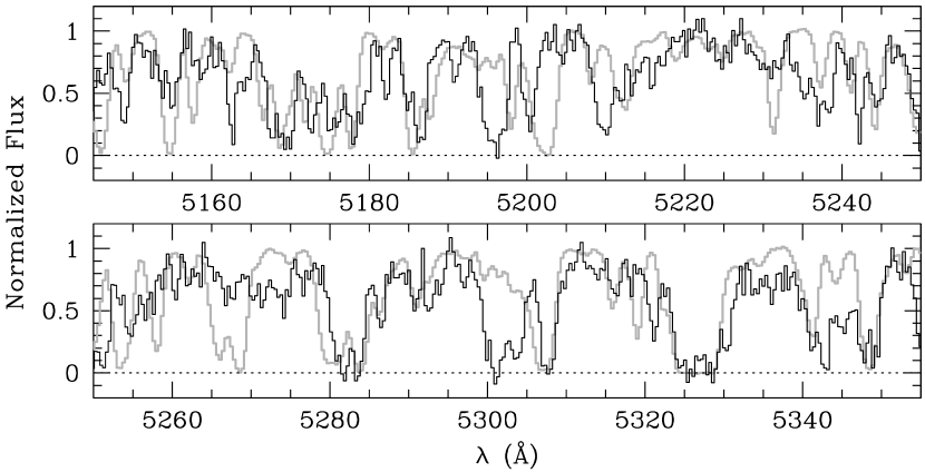
Figure 3: A representative section of the Ly$\alpha$ forest in the normalized spectra of Q1422 (grey line) and Q1424 (black line).

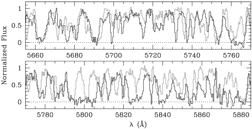
Figure 4: Same as Figure 3, here for Q1439A (grey line) and Q1439B (black line).

A visual comparison of the Ly$\alpha$ forest in the paired spectra suggests that the most striking similarity occurs among the strongest absorption features (see Figures 3 and 4). These regions often appear to be similar along adjacent lines of sight, as do regions where the absorption is nearly zero (possible “voids” relatively free of absorbing material). Matches among intermediate strength features are less obvious, which suggests that the structures giving rise to those lines may not be as coherent over the separation between sightlines. However, many strong lines and regions of nearly zero absorption that do not coincide between spectra can also be identified. The alignment of a subset of features may occur purely by chance.

Our spectral coverage also allows us to investigate the extent to which metal systems span parallel lines of sight. Two strong C iv systems appear toward Q1439B at $z\approx 3.4$, separated by 1700 km s^-1. Each system has a large rest equivalent width, $W_{\rm rest}(1548)\sim 1.5$ Å. However, no C iv appears at this redshift toward Q1439A. In contrast, a low-ionization system containing Mg ii and Fe ii does appear along both sightlines at $z\approx 1.68$, separated by only $\sim 400$ km s^-1. A single, extended absorber responsible for the low-ionization features would have a linear size $\gtrsim 280$ $h_{70}^{-1}$ proper kpc. These lines may alternatively arise from the chance intersection of separate, clustered absorbers. Weaker C iv systems appear in both Q1422 and Q1424 separated by $\sim 440$ km s^-1 at $z\approx 3.08$, where the separation between sightlines is 290 $h_{70}^{-1}$ proper kpc. We expand further on the properties of metal systems in the appendix.

In order to assess the impact of spectral characteristics on our Ly$\alpha$ forest results we additionally employed a deep, high-resolution spectrum of Q1422+2309A. Observations were made with the Keck High Resolution Echelle Spectrometer (HIRES) (Vogt et al., 1994) using a 0$\farcs$574 slit. This yields a spectral resolution FWHM = 4.4 km s^-1. Reductions were performed as described Rauch, Sargent, & Barlow (2001). In addition to the data from that work, which used the red cross-disperser only, we include subsequent exposures taken with the UV-blazed cross-disperser installed to provide additional coverage of the Ly$\alpha$ forest. The final spectrum was binned to give a constant velocity width for each pixel of 2.1 km s^-1, with a typical S/N per resolution element of $50-90$.

3 Comparison of Sightlines

3.1 Correlation Functions

The correlation of transmitted flux in the spectra of closely separated quasars provides a simple means of quantifying the degree of similarity in the matter distribution along adjacent sightlines. We define the unnormalized correlation, $\xi$, of the spectra of two sources separated on the sky by an angle $\Delta\theta$ as

$$\xi(\Delta\theta,\Delta v_{\|})=\frac{1}{N}\sum[F(\Delta\theta,v_{\|}+\Delta v_{\|})-\bar{F}(\Delta\theta)][F(0,v_{\|})-\bar{F}(0)],$$ (3)

where $F$ is the continuum-normalized flux, $\bar{F}(\Delta\theta)$ and $\bar{F}(0)$ are the mean fluxes along the two sightlines, $v_{\|}$ is the line-of-sight velocity, $\Delta v_{\|}$ is the longitudinal velocity lag, and $N$ is the total number of pixels in each spectrum within the region of interest. The sum is performed over all available pixels at a given velocity lag, of which there will be

$$n_{\rm pix}(\Delta v_{\|})=N-\Delta v_{\|}/\delta v_{\rm pix}$$ (4)

for a pixel size $\delta v_{\rm pix}$. The normalized correlation value can be computed by dividing Eq. (3) by the standard deviation in each input spectrum.

We have chosen a pixel size for the combined spectra to give roughly 3 pixels/resolution element. However, we note that the $1/N$ factor in Eq. (3) implies that the value of the correlation will be insensitive to pixel size so long as the spectrum is well sampled. The increase in the sum created by using a larger number of smaller pixels will be offset by the increase in $N$ so long as there are $\gtrsim 2$ pixels/resolution element. Using pixels larger than the spectral resolution will introduce smoothing effects (see §4).

In order to assess the coherence of absorbing structures across adjacent sightlines, we compute the crosscorrelation of transmitted flux in the Ly$\alpha$ forest in the spectra of our quasar pairs. As a reference, we also determine the autocorrelation, $\xi(0,\Delta v_{\|})$, along lines of sight toward individual objects. At these high redshifts, H i Ly$\alpha$ absorption will strongly dominate over contaminating absorption from lower-redshift metals such as C iv and Mg ii. The correlation functions should therefore accurately reflect the distribution of neutral hydrogen to within the present measurement errors. All correlations are computed in single-pixel steps, which are 20 km s^-1 for the ESI data. Figure 5 displays the autocorrelation function for each quasar along with the crosscorrelation functions between adjacent sightlines. Both in the case of Q1422/Q1424 and Q1439A/B, a clear peak in the crosscorrelation at zero lag indicates a genuine similarity between sightlines.

Undulations in the correlation functions arising from the chance superposition of unrelated lines constitute the dominant source of uncertainty in the peak values (see discussion on photon noise below). Pixel-to-pixel variations in the correlations are themselves clearly correlated. However, we find that the overall distributions of values away from the central peaks are very nearly Gaussian. We therefore take the standard deviation of pixels in the “noise” region, which we define to be where 2000 km s^-1 $\leq|\Delta v_{\|}|\leq$ 18000 km s^-1, as the $1\sigma$ error in a correlation peak value. In this region we expect no underlying signal, however the correlation is still computed from at least half of the available pixels. Since the sum in Eq. (3) is computed over fewer pixels as the velocity lag increases, yet the factor $1/N$ remains constant, the amplitude of the noise features will tend to diminish as $\sqrt{n_{\rm pix}(\Delta v_{\|})}$, where $n_{\rm pix}(\Delta v_{\|})$ is the number of pixels included in the sum in Eq. (3) at lag $\Delta v_{\|}$. Therefore, in order to match the amplitude of the noise at $\Delta v_{\|}=0$, we multiply the correlation at each lag by a scale factor $s$ before computing the standard deviation, where

$$s=\sqrt{\frac{n_{pix}(0)}{n_{\rm pix}(\Delta v_{\|})}}=\sqrt{\frac{N}{N-\Delta v_{\|}/\delta v_{\rm pix}}}.$$ (5)

For the range in velocity lag defined above this is a modest correction. Including only lags where at least half of the $\sim 1800$ Ly$\alpha$ pixels in each spectrum overlap limits $s$ to at most $\sqrt{2}$. For the range in velocity lag shown in Fig. 5, $s<1.2$.

Our results for the crosscorrelations are summarized in Table 2. Using the above estimate for the error, the peak in the crosscorrelation for Q1422/Q1424 (Q1439A/B) is significant at the $7\sigma$ ($5\sigma$) level. This strongly suggests coherence in the absorbing structures on the scale of the $230-300$ $h_{70}^{-1}$ proper kpc transverse separation between sightlines. The marginal consistency of the peak values with one another likely reflects the similarity in sightline separation and redshift for the two quasar pairs. The zero-lag values of the autocorrelations, which give the variance in the flux for these sections of the Ly$\alpha$ forest, are 0.0950 for Q1422, 0.0796 for Q1424, 0.0862 for Q1439A, and 0.1000 for Q1439B. Thus, the normalized crosscorrelation peaks are $41.2\pm 5.7\%$ for Q1422/Q1424 and $31.9\pm 6.2\%$ for Q1439A/B.

3.2 Flux Distributions

The flux crosscorrelations demonstrate that at least some Ly$\alpha$ absorbers span the separation between our paired lines of sight. However, it does not indicate whether the similarity between sightlines depends on the strength of the absorber. The crowded nature of the Ly$\alpha$ forest at $z\sim 4$, together with the present spectral resolution, greatly inhibits a study of individual lines. However, we are able to look at the agreement between absorption features on a pixel-by-pixel basis.

Our goal is to determine whether the similarity in flux between paired spectra depends on the amount of absorption for an individual pixel. First we first select those Ly$\alpha$ forest pixels in one spectrum (Q1422 or Q1439A) whose flux falls within a specified range. We then identify the pixels in the companion spectrum with matching wavelengths and compute their flux distribution. Comparing the distribution in this subsample to that in all Ly$\alpha$ forest pixels in the companion spectrum allows us to evaluate whether there exists an overabundance of pixels in the specified flux range relative to that expected on random chance.

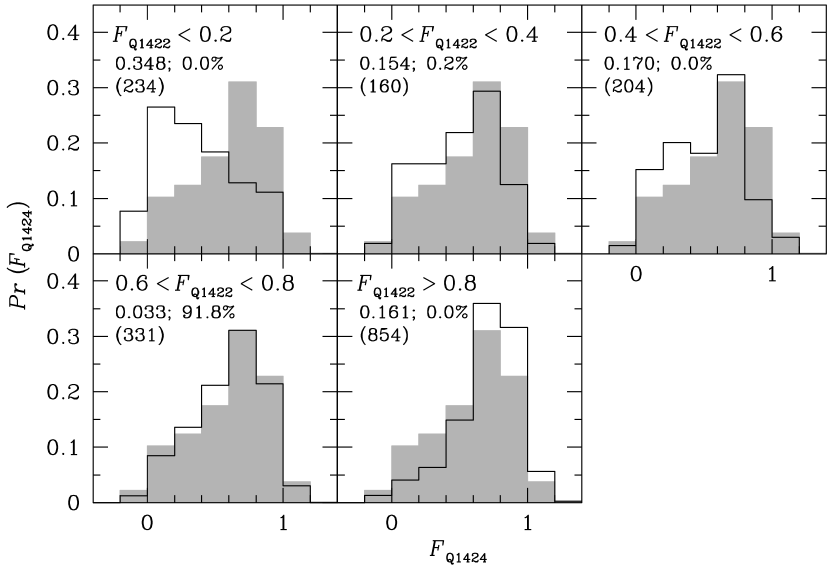
Figure 6: Distributions of continuum-normalized pixel fluxes in the Ly$\alpha$ region of Q1424 as a function of the flux in Q1422. Unshaded histograms show the flux probability distribution for the subsample of pixels in Q1424 corresponding in wavelength to those pixels in Q1422 that have fluxes in the indicated range. Shaded histograms show the probability distribution for all Q1424 pixels in the Ly$\alpha$ region. For each range of flux in Q1422, the two-sided Kolmogorov-Smirnov statistic for the subsample and full sample of Q1424 flux values is presented along with the associated likelihood, expressed as a percent, of obtaining a higher value if the the two samples were drawn from the same distribution. The number of pixels in each subsample is given in parentheses. The full sample contains 1783 pixels.

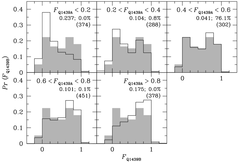
Figure 7: Same as Figure 6, here for pixel fluxes in the Ly$\alpha$ region of Q1439B as a function of the flux in Q1439A. The full sample contains 1793 pixels.

The results for Q1422/Q1424 and Q1439A/B are shown in Figures 6 and 7, respectively. Each panel shows the normalized distribution of Q1424 or Q1439B pixels in the indicated subsample along with the distribution of all Ly$\alpha$ forest pixels in that spectrum. The range of flux in Q1422 or Q1439A for each subsample is chosen to be significantly larger than the typical flux uncertainty. In each case, we compute the two-sided Kolmogorov-Smirnov statistic, which is the maximum difference between the cumulative fractions of pixels in the subsample and of all pixels in the forest, along with the associated likelihood of randomly obtaining a smaller statistic than the one observed. The number of pixels in each subsample is also shown.

The clearest results occur at extreme levels of absorption. Pixels in Q1422 (Q1439A) either near saturation, $F<0.2$, or near the continuum, $F>0.8$, tend to strongly coincide with pixels of similar flux in Q1424 (Q1439B). Intermediate flux pixels appear to be less strictly matched, with the exception of pixels in Q1422 with $0.4<F<0.6$. For certain subsamples, namely $0.6<F<0.8$ in Q1422 and $0.4<F<0.6$ in Q1439A, the distribution of fluxes in the companion spectrum is consistent with a random selection. This seems to confirm the visual appraisal that strong absorbers and regions relatively free of absorbing material tend to span adjacent lines of sight more readily than do absorbers of intermediate strength.

While each sample includes enough pixels to produce a statistically significant result, a few caveats are worth considering. Systematic errors in continuum fitting might artificially create clusters of pixels with low absorption near the same wavelength in pairs of spectra. Similarly, errors in sky-subtraction that are repeated between spectra might create false coincidences of pixels near zero flux. Multiple independent continuum fits resulted in typical differences of $\sim 10\%$ in flux on scales of $\sim 100$ Å. We likewise find no evidence for large systematic errors in the sky subtraction. Given that the resulting uncertainties are significantly smaller than the range in flux used to define a subsample in Figures 6 & 7, these effects should only be a minor concern.

We stress that comparing transmitted fluxes does not strictly yield a clear physical interpretation. Pixels of intermediate flux commonly occur along the wings of strong features. They will therefore tend to cluster less readily than pixels near the continuum or near saturation, especially if the strong lines shift in velocity between spectra. Moreover, agreement in flux does not necessarily indicate agreement in optical depth. Since transmitted flux decreases exponentially with optical depth, $\tau$, the difference in flux for a given fractional change in $\tau$ will depend on the value of $\tau$ itself. For a small characteristic change between sightlines, $\Delta\tau/\tau\ll 1$, the greatest scatter in flux is expected for $\tau\sim 1$, with the scatter decreasing as $\tau\rightarrow 0$ or as $\tau\rightarrow\infty$. Therefore, it is unclear whether the enhanced agreement in flux among pixels with flux near the continuum or near saturation indicates that the corresponding gas is more homogeneous on these scales than the gas giving rise to intermediate absorption features. More specific insights may be drawn by comparing our measured flux distributions to those derived from numerical simulations.

4 Effects of Photon Noise and Instrumental Resolution

Comparing the longitudinal and transverse flux correlation functions (or power spectra, equivalently) in the Ly$\alpha$ forest has been been explored by several authors as a means of measuring the cosmological geometry via the Alcock-Paczyński test. This application primarily requires a sample of sightlines large enough to overcome cosmic variance. However, some question remains regarding the dependence of the correlation functions on data characteristics such as signal-to-noise ratio and resolution. It is particularly important to know to what extent the autocorrelation measures the physical correlation length along the line of sight rather than the instrumental resolution. For additional discussion on the effects of spectral characteristics see, e.g., Lin & Norman (2003) and Croft et al. (1998).

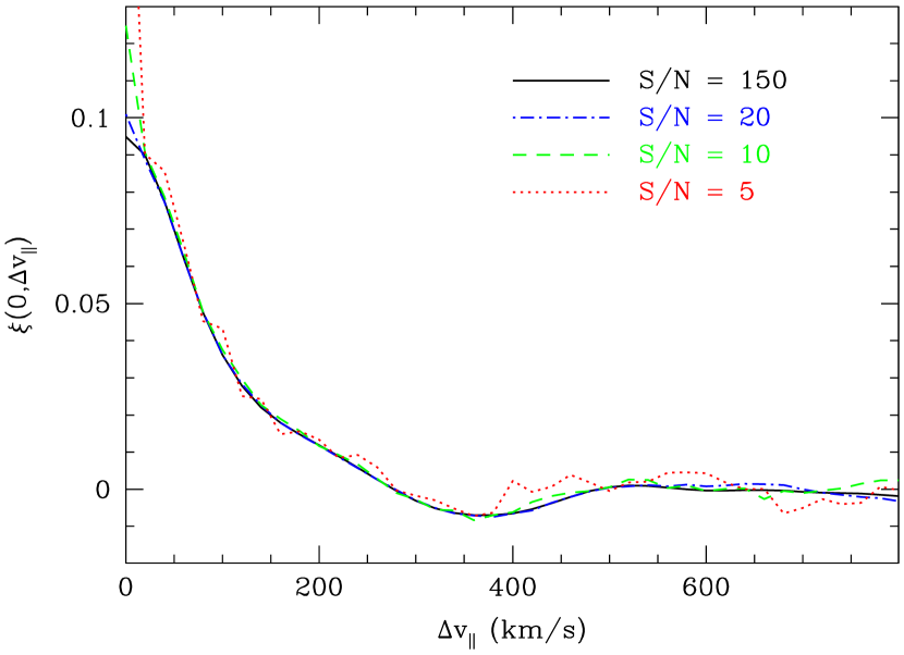
Figure 8: The effects of photon noise on the shape of the autocorrelation function. The solid line shows the autocorrelation computed from our original ESI spectrum of Q1422 (FWHM = 55 km s^-1, S/N = 150 per resolution element). Additional lines show the autocorrelation recomputed after adding random Gaussian noise to the original spectrum such that the resulting S/N per resolution element is 20 (dash-dotted line), 10 (dashed line), and 5 (dotted line). Autocorrelation functions were computed in longitudinal velocity lag steps of 20 km s^-1. The spike at $\Delta v_{\|}=0$ reflects only a single point for each curve.

In the preceding analysis we assumed that the chance alignment of unrelated absorption features dominated over photon noise in producing uncertainty in the flux correlations. To justify this, we recomputed the autocorrelation for the ESI spectrum of Q1422 after adding increasing levels of Gaussian random noise. The results appear nearly identical for S/N $\gtrsim 10$ per resolution element (Figure 8). A spike at $\Delta v_{\|}=0$ appears in the autocorrelation function as the variance in the noise becomes comparable to the intrinsic variance in the absorption features. However, no such jump is expected to occur in the crosscorrelation since the photon noise in the two spectra should be uncorrelated. Large sets of moderate S/N spectra may therefore be more useful than smaller sets of high S/N for this type of work.

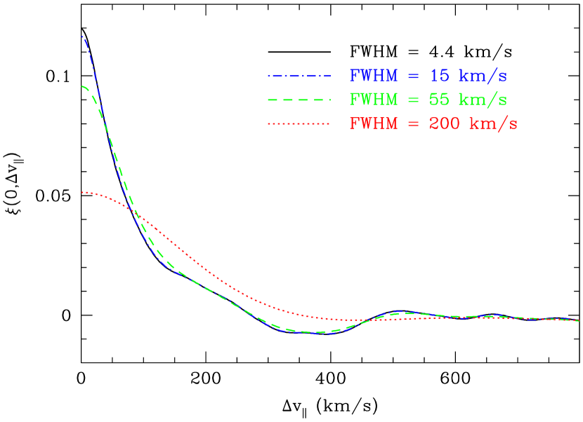
Figure 9: The effects of spectral resolution on the shape of the autocorrelation function. The solid line shows the autocorrelation computed from our original HIRES spectrum of Q1422 (FWHM = 4.4 km s^-1). Additional lines show the autocorrelation recomputed after smoothing the HIRES data to a spectral resolution FWHM of 15 km s^-1 (dash-dotted line), 55 km s^-1 (dashed line), and 200 km s^-1 (dotted line).

To address the effects of spectral resolution on the autocorrelation we have synthesized moderate- and low-resolution spectra from a high-quality Keck HIRES spectrum of Q1422 (resolution FWHM = 4.4 km s^-1). In each test case we first tune the spectral resolution by convolving the HIRES data with a Gaussian kernel and then compute the resulting autocorrelation function. The results for spectra with resolution FWHM = 4.4 (unsmoothed), 15, 55, and 200 km s^-1 are plotted in Figure 9. Very little difference exists between the autocorrelation functions computed from the unsmoothed HIRES data and from the data smoothed to FWHM = 15 km s^-1. Thus, we may conclude that the correlation in the unsmoothed HIRES data is an accurate measure of the intrinsic correlation in the Ly$\alpha$ forest (subject to cosmic variance and redshift-space distortions). The Ly$\alpha$ lines are already smoothed by their thermal width and easily resolved with HIRES. However, when the spectrum is degraded to FWHM = 55 km s^-1, similar to ESI data, the autocorrelation is clearly broadened and diminished in amplitude. (We note that the autocorrelation measured from this “synthetic” ESI spectrum is nearly identical to that computed from the real ESI data.) At even lower resolution, comparable to Keck/LRIS or VLT/FORS2, the spectral resolution dominates over the intrinsic correlation length.

As the spectral resolution decreases, the peak of the autocorrelation also incorporates more of the outlying noise (random undulations in the correlation function at $\Delta v\gg 0$). At large velocity lags ($\Delta v_{\|}\gg 200$ km s^-1), disagreement between the high-resolution and low-resolution cases may be due in part to these noise features. Better agreement may result when the correlation function is averaged over many sightlines.

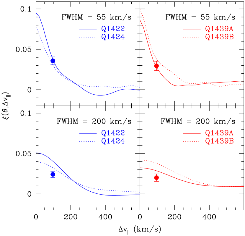
Figure 10: The relative effects of spectral resolution on auto- and crosscorrelations. Top panels: Autocorrelation functions computed from the Ly$\alpha$ regions in the indicated unsmoothed ESI spectra (FWHM = 55 km s^-1) (solid and dotted lines) overlaid with the peak value of the crosscorrelation computed between those spectra (filled circles). The peak of the crosscorrelation is plotted at a velocity lag equal to the transverse separation between the two lines of sight for the case of $\Omega_{m}$= 0.3, $\Omega_{\Lambda}$= 0.7, and $H_{0}=70$ km s^-1 Mpc^-1. Bottom panels: Same as the top panels, here after smoothing the ESI spectra to a resolution of 200 km s^-1.

A more subtle issue is how spectral resolution affects the agreement between autocorrelation and crosscorrelation functions. To address this, we degraded the resolution of our ESI data to mimic observations using a lower resolution instrument (FWHM = 200 km s^-1) and then recomputed the correlations. Figure 10 contrasts the results from the original spectra with those from the smoothed versions. In each case we plot the autocorrelation functions computed from single sightlines and overplot the peak of the corresponding crosscorrelation at a velocity lag equal to the transverse velocity separation between the lines of sight ($\Delta v_{\bot}=98$ km s^-1 for Q1422/Q1422, $\Delta v_{\bot}=96$ km s^-1 for Q1439A/B for the case of $\Omega_{m}$= 0.3, $\Omega_{\Lambda}$= 0.7, and $H_{0}=70$ km s^-1 Mpc^-1).

The differences shown in Figure 10 between the ESI and low-resolution cases suggest a significant dependence on spectral resolution. At ESI resolution the concordance between auto- and crosscorrelations appears to be very good for both pairs of sightlines. However, at low resolution the peaks of the crosscorrelation functions fall well below the values of the autocorrelation functions at the same total velocity separation. While part of this effect may be due to noise in the correlations, the general dependence on resolution can be understood in regions where the intrinsic correlation function is non-linear on scales smaller than the width of the smoothing kernel. (This includes the region around the peak at zero lag, since the correlation is expected to be symmetric about $\Delta v_{\|}=0$.) Convolving the input spectra with a smoothing kernel produces a correlation function that has been convolved twice with the same kernel, once for each spectrum. The resulting unnormalized autocorrelation function may therefore be higher or lower at a particular velocity lag, depending on the shape of the correlation function at that point. However, since the peak of the crosscorrelation function is already a maximum it can only decrease as a result of smoothing (apart from the effects of noise). Thus, if we adjust our cosmology such that, at high spectral resolution, the composite crosscorrelation function built up from pairs at many different separations agrees with the mean autocorrelation function (ignoring redshift-space distortions), then this agreement may not hold when using low-resolution data. Spectral resolution must therefore be considered carefully when performing this type of comparison, for example by referring to artificial spectra drawn from numerical simulations of large-scale structure.

5 Conclusions

We have analyzed the transverse properties of the Ly$\alpha$ forest at $3.0\lesssim z\lesssim 4.1$ on scales of $\sim 1$ $h_{70}^{-1}$ comoving Mpc ($230-300$ $h_{70}^{-1}$ proper kpc) toward the $z\approx 3.63$ quasar pair Q1422+2309A/Q1424+2255 and the $z\approx 4.25$ pair Q1439-0034A/B. Strong peaks at zero velocity lag in the flux crosscorrelations between paired sightlines indicate coherence in the H i absorbers on these scales. The crowded nature of the Ly$\alpha$ forest at these redshifts restricts a line-by-line comparison. However, a statistical approach suggests that the flux in paired spectra tends to be most similar in regions of either very strong or very weak absorption. The similarities at flux levels near the continuum are consistent with the large sizes of voids and low-density gaseous filaments and sheets expected to comprise much of the intergalactic medium. The more surprising similarities at low flux levels may simply reflect the limited dynamic range of transmitted flux in distinguishing among regions of high optical depth ($\tau\gg 1$). Larger differences in flux found at intermediate flux levels may relate to the increased scatter in flux naturally expected for optical depths near unity, and also to the fact that flux differences along the wings of strong lines will be sensitive to bulk velocity shifts between sightlines. Despite the difficulty in producing a clear physical interpretation from the data alone, both the correlation and flux statistics should provide a useful resource for comparison with numerical simulations.

In order to assess the dependence of the correlation functions on photon noise and spectral resolution we have employed high-quality ESI and HIRES spectra of Q1422. Adding photon noise has very little effect for S/N $\gtrsim 10$ per resolution element except to introduce a spike in the autocorrelation at zero lag. Increasing the resolution FWHM increases the velocity width of the autocorrelation and decreases its amplitude, as expected. These effects may occur unevenly, however, due to the incorporation of noise features as the peak broadens. We further tested the effects of resolution on the relative amplitudes of the autocorrelation and crosscorrelation by degrading the resolution of our ESI spectra to match that of a low-resolution spectrograph such as Keck/LRIS or VLT/FORS2. For both pairs, the crosscorrelation and autocorrelations agree well for our adopted cosmology when the correlations are computed from the original ESI data. However, smoothing the spectra substantially reduces the crosscorrelation with respect to the autocorrelations. This will typically occur at any velocity lag where the intrinsic correlation function is non-linear on scales smaller than the width of the smoothing kernel. Cosmological tests making use of the Ly$\alpha$ forest correlation length should take this effect into account.

Finally, we present an inventory of metal lines in Q1424, Q1439A, and Q1439B in the appendix. The most noteworthy features are a pair of strong C iv complexes at $z\approx 3.4$ appearing only toward Q1439B. Given their large equivalent widths, the relatively small separation between these systems suggests that they are related, possibly arising from separate galaxy halos or two sides of a galactic outflow. Low-ionization systems containing Mg ii and Fe ii appear at $z\approx 1.68$ in Q1439 A and B separated by 410 km s^-1. These may either represent a single, extended structure ($\Delta l\gtrsim 280$ $h_{70}^{-1}$ proper kpc) or separate, clustered absorbers. A C iv system appears toward Q1424 at $z=3.084$, within 440 km s^-1 of a known C iv system toward Q1422. A single absorber responsible for both systems would have a transverse size $\gtrsim 290$ $h_{70}^{-1}$ proper kpc. However, the number density of weak C iv systems at this redshift suggests that these lines may instead result from chance superposition.

Appendix A Metal Systems

Previous studies using quasar pairs and multiply-imaged lensed quasars have demonstrated spatial coherence in metal systems over a variety of length scales. Differences between metal systems in narrowly-separated lines of sight suggest that the absorbers giving rise to individual lines seen in high-resolution spectra span at most a few kiloparsecs, both for high-ionization systems seen in C iv and for low-ionization systems seen in Mg ii (Lopez et al., 1999; Petitjean et al., 2000; Rauch, Sargent, & Barlow, 2001; Rauch et al., 2002; Churchill et al., 2003; Tzanavaris & Carswell, 2003; Ellison et al., 2004). However, these absorbers may be part of larger structures extending $\gtrsim 20$ $h_{70}^{-1}$ kpc (Smette et al., 1995) and even $\gtrsim 100$ $h_{70}^{-1}$ kpc for highly ionized material (Petitjean et al., 1998; Lopez et al., 1999; Lopez, Hagen, & Reimers, 2000).

The present data afford us a unique opportunity to probe the coherence of metal systems on scales of $\sim 300$ $h_{70}^{-1}$ proper kpc. Unfortunately, modest signal-to-noise and significant contamination from skylines in the red part of our spectra greatly limit our sensitivity and hinder completeness estimates. Our detections are limited to relatively strong lines and lines that fall in regions of unusually high S/N.

Line lists for Q1424, Q1439A, and Q1439B are presented in Tables 3, 4, and 5, respectively. In the following sections we briefly comment on some of the more interesting systems. Results for Q1422 are presented in detail elsewhere (Rauch, Sargent, & Barlow, 2001; Bechtold & Yee, 1995; Petry, Impey, & Foltz, 1998). For each line we measure the wavelength centroid and equivalent width. Weighted mean redshifts are given where multiple lines are measured for a single ion. In the case of blended lines we attempt to alleviate the overlap by fitting Voigt profiles to any unblended transitions of the same ions using VPFIT and then dividing by the inferred model profiles. This typically allows us to obtain values for at least the strongest blended components.

A.1 Q1424+2255

Strong associated broad absorption lines (BALs) at $z=3.62$ are seen in C iv and N v along with weaker associated absorption in Si iv (although the Si iv appears affected by skyline contamination). Isolated components of C iv and N v appear up to 1000 km s^-1 blueward of the BAL. These suggest small pockets of outflowing material moving at a higher velocity than the material responsible for the bulk of the broad absorption. C iv is also seen at $z=3.62$ toward Q1422A. (Rauch, Sargent, & Barlow, 2001). However, since the absorption is associated with the quasar in both cases, these features are unlikely to be related.

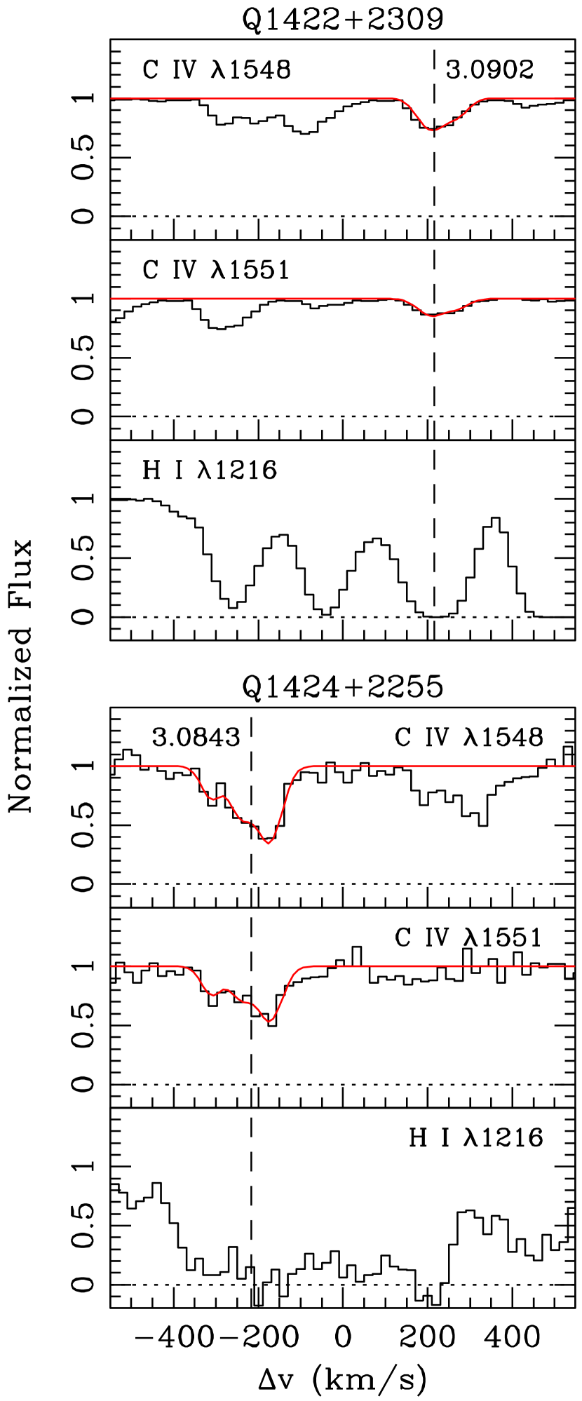
Figure 11: Top three panels: Continuum-normalized ESI spectrum of Q1422 (histogram) showing the C iv and H i absorption for the system at $z=3.0902$ reported by Rauch, Sargent, & Barlow (2001). The continuous lines show the Voigt profile fits computed from HIRES data where the profiles have been smoothed to ESI resolution. Bottom three panels: Continuum-normalized ESI spectrum of Q1424 (histogram) showing the C iv and H i absorption for the system measured herein at $z=3.0843$. The continuous lines show Voigt profile fits computed from the ESI data. All components in both spectra are placed on a common velocity scale in order to demonstrate the longitudinal velocity separation between these systems.

An intervening C iv system appears at $z=3.084$. We additionally identify the line at 5692.3 Å to be Si iv $\lambda$1394 at the same redshift, where Si iv $\lambda$1403 is blended with N v $\lambda$1239 at $z=3.621$. A C iv complex with possible Si iv appears at $z=3.090$ toward both the A and C images of Q1422 (Rauch, Sargent, & Barlow, 2001; Boksenberg, Sargent, & Rauch, 2003), implying a transverse size $\gtrsim 290$ $h_{70}^{-1}$ proper kpc for a single structure spanning all three lines of sight. Figure 11 shows the C iv absorption at this redshift in Q1424 and Q1422. The systems are narrowly separated along the line of sight, with $\Delta v\approx 440$ km s^-1. However, Boksenberg, Sargent, & Rauch (2003) find $\sim 25$ C iv systems per unit redshift at $z=3$ for systems with total column density $N_{\rm syst}({\rm C\;\mbox{\tiny IV}})>10^{12}$ cm^-2. This translates to a typical spacing between systems of only $\sim 3000$ km s^-1. It is therefore reasonable to suspect that this superposition of relatively modest C iv absorbers toward Q1422 and Q1424 occurs by chance. Significant H i absorption occurs along both lines of sight in the velocity interval spanned by these systems, though this may be due to the crowded state of the Ly$\alpha$ forest at $z\sim 3$.

A.2 Q1439-0034A & B

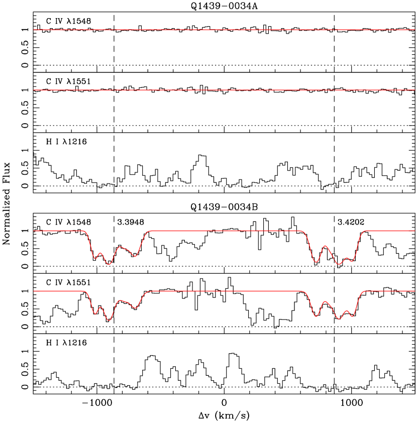
Figure 12: Top three panels: Continuum-normalized ESI spectrum of Q1439A (histogram) covering the C iv and H i regions near $z=3.4$. The continuous lines in the top two panels demonstrate the absence of C iv over this interval. Bottom three panels: Continuum-normalized spectrum of Q1439B (histogram) showing the C iv and H i absorption for the systems at $z=3.3948$ and $z=3.4202$. The continuous lines show the Voigt profile fits to the C iv absorption. Several of the C iv $\lambda$1548 pixels near 850 km s^-1 in this plot are heavily affected by skylines and have been excluded from the fit. All components in both spectra are placed on a common velocity scale in order to demonstrate the longitudinal velocity separation between these systems.

Two broad C iv complexes at $z\approx 3.4$ form the most conspicuous metal absorption features in the spectrum of Q1439B (Figure 12). The systems are separated by 1700 km s^-1, and each has a velocity width of $\sim 400$ km s^-1. Neither complex is observed toward Q1439A. The individual components are unlikely to be resolved with ESI. However, we can place a lower limit on the column density of these systems by assuming that the weaker transition (C iv $\lambda$1551) falls on the linear part of the curve-of-growth. In that case, the column density, $N_{\rm syst}$, is related to rest equivalent with, $W_{\rm rest}$, as

$$W_{\rm rest}=\frac{\pi e^{2}}{m_{e}c^{2}}f\lambda_{0}^{2}N_{\rm syst},$$ (A1)

for a transition with rest wavelength $\lambda_{0}$ and oscillator strength $f$. For the lower-equivalent width system ($z_{\rm abs}=3.402$, $W_{\rm rest}(1551)\approx 1.1$ Å), this gives $N_{\rm syst}({\rm C\;\mbox{\tiny IV}})\gtrsim 5\times 10^{14}$ cm^-2. If we adopt a power-law column density distribution $d^{2}{\cal N}/dN_{\rm syst}dz\propto N_{\rm syst}^{-\beta}$, where ${\cal N}$ is the number of systems, then we would expect $\lesssim 0.6$ systems per unit redshift in this column density range based on the above Boksenberg et al. (2003) results and adopting their value of $\beta=1.6$. The narrow redshift spacing of these two systems ($\Delta z=0.025$) therefore strongly suggests that they are related. One explanation is that the absorption complexes arise from two sides of an intervening galactic outflow. Alternatively, the high levels of H i absorption seen at both C iv redshifts may indicate a pair of galaxy halos.

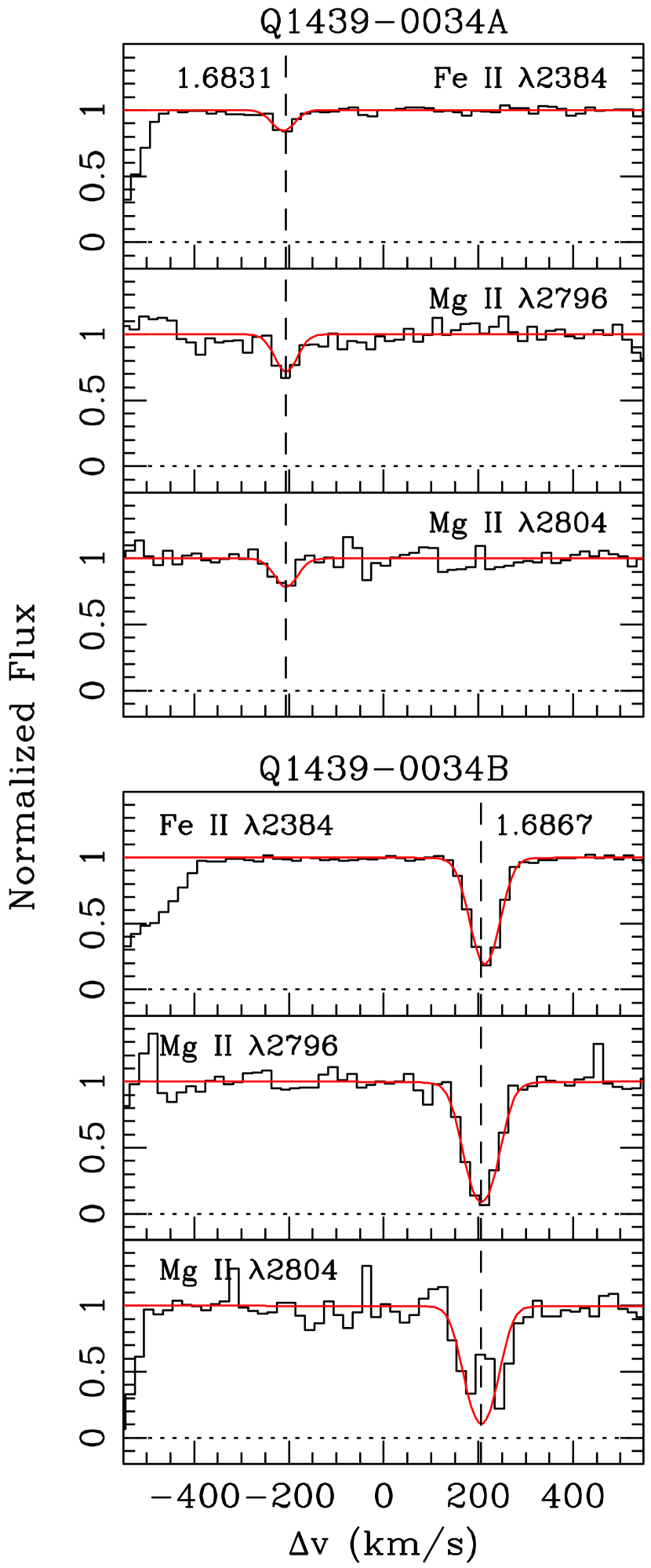
Figure 13: Top three panels: Continuum-normalized spectrum of Q1439A (histogram) showing the Mg ii and Fe ii absorption for the system at $z=1.6831$. The continuous lines show Voigt profile fits. Bottom three panels: Same as the top panels, here for the system at $z=1.6867$ in Q1439B. Several of the Mg ii $\lambda$2804 pixels in Q1439B near 200 km s^-1 in this plot are heavily affected by skylines and have been excluded from the fit. All components in both spectra are placed on a common velocity scale in order to demonstrate the longitudinal velocity separation between these systems.

Mg ii + Fe ii systems appear toward both Q1439 A and B at $z\approx 1.68$, separated between spectra by 410 km s^-1 along the line of sight (Figure 13). From Churchill et al. (1999), the number of Mg ii systems per unit redshift with rest equivalent width $W_{\rm rest}(2796)>0.02$ Å is expected to be $\approx 2.7$. The probability of randomly finding a system within this velocity separation is therefore $\sim 0.02$, or a factor of three lower if we restrict ourselves to strong ($W_{\rm rest}(2796)>0.3$) systems (Steidel & Sargent, 1992). Thus, there is a high likelihood that these systems are related. Both Mg ii and Fe ii appear stronger toward B than toward A, with a factor of seven difference between sightlines in the equivalent widths of Mg ii $\lambda$2804 and Fe ii $\lambda$2384. These features may arise either from a single absorber spanning the 280 $h_{70}^{-1}$ proper kpc between sightlines or from a pair of clustered objects. Two additional strong Mg ii systems appear along only a single sightline, one toward A at $z=2.266$ and another toward B at $z=1.399$.

Q1439B is a BAL quasar showing high levels of associated absorption in C iv and N v. We identify the O i absorption reported by Fukugita et al. (2004) as the strong C iv systems at $z\approx 3.4$ mentioned above. No strong associated absorption is seen for Q1439A. As noted by Fukugita et al. (2004), the difference in associated absorption features supports the hypothesis that Q1439 A and B are a true binary and not a lensed pair.

Table 1: Summary of Observations

Object	Date	Exp. time	FWHM
		(s)	(km s-1)
Keck/ESI
Q1422+2309A	2000 Mar 03-04	1200	$\sim 55$
Q1424+2255	2000 Mar 03 – 2001 Apr 21	44900	$\sim 55$
Q1439-0034A	2001 Jan 26 – 2002 Jun 10	8000	$\sim 55$
Q1439-0034B	2001 Apr 19 – 2002 Jun 10	42400	$\sim 55$
Keck/HIRES
Q1422+2309A	1998 Jan 30 – 1998 Apr 15	31600	4.4

Table 2: Ly$\alpha$ Forest Crosscorrelation Values

QSO Pair	$\Delta\theta$	$z_{{\rm Ly}\alpha}$	$\Delta l$	$\Delta v_{\bot}$	$\xi(\Delta\theta,0)$
			$h_{70}^{-1}$ proper kpc	km s-1	Unnormalized	Normalized
Q1422/Q1424	$38\farcs 5$	$2.965-3.466$	$283-298$	97.8	$0.0358\pm 0.0049$	$0.412\pm 0.057$
Q1439A/B	$33\farcs 4$	$3.496-4.075$	$230-245$	96.3	$0.0296\pm 0.0057$	$0.319\pm 0.062$

Table 3: Q1424+2255 Metal Systems

$\lambda_{\rm obs}$	Line ID	$z_{\rm obs}$	$W_{\rm rest}$
(Å)			(Å)
Intervening
$5692.34\pm 0.12$	Si iv $\lambda$1394	$3.08417\pm 0.00009$	$0.29\pm 0.02$
$6323.34\pm 0.14$	C iv $\lambda$1548	$3.08433\pm 0.00007$	$0.50\pm 0.03$
$6333.93\pm 0.17$	C iv $\lambda$1550	$3.08433\pm 0.00007$	$0.37\pm 0.03$
Associated
$5704.76\pm 0.08$	N v $\lambda$1239	$3.60499\pm 0.00007$	$0.34\pm 0.01$
$5709.70\pm 0.11$	N v $\lambda$1239	$3.60898\pm 0.00009$	$0.11\pm 0.01$
$5724.81\pm 0.08$	N v $\lambda$1239	$3.62118\pm 0.00005$	$0.96\pm 0.02$
$5743.22\pm 0.09$	N v $\lambda$1243	$3.62118\pm 0.00005$	$0.75\pm 0.02$
$6437.34\pm 0.17$	Si iv $\lambda$1394	$3.61865\pm 0.00009$	$0.24\pm 0.03$
$6478.79\pm 0.21$	Si iv $\lambda$1403	$3.61865\pm 0.00009$	$0.16\pm 0.02$
$7129.64\pm 0.08$	C iv $\lambda$1548	$3.60511\pm 0.00005$	$0.36\pm 0.01$
$7135.69\pm 0.16$	C iv $\lambda$1548	$3.60902\pm 0.00010$	$0.10\pm 0.01$
$7141.28\pm 0.08$	C iv $\lambda$1550	$3.60511\pm 0.00005$	$\lesssim 0.37$
$7144.70\pm 0.13$	C iv $\lambda$1548	$3.61484\pm 0.00008$	$0.08\pm 0.01$
$7153.99\pm 0.07$	C iv $\lambda$1548	$3.62085\pm 0.00004$	$1.82\pm 0.03$
$7165.96\pm 0.11$	C iv $\lambda$1550	$3.62085\pm 0.00004$	$1.44\pm 0.06$

Table 4: Q1439-0034A Metal Systems

$\lambda_{\rm obs}$	Line ID	$z_{\rm obs}$	$W_{\rm rest}$
(Å)			(Å)
Intervening
$6393.06\pm 0.10$	Fe ii $\lambda$2383	$1.68304\pm 0.00004$	$0.07\pm 0.01$
$7502.82\pm 0.12$	Mg ii $\lambda$2796	$1.68305\pm 0.00004$	$0.18\pm 0.02$
$7521.87\pm 0.19$	Mg ii $\lambda$2804	$1.68305\pm 0.00004$	$0.10\pm 0.02$
$9134.29\pm 0.14$	Mg ii $\lambda$2796	$2.26645\pm 0.00004$	$0.30\pm 0.03$
$9157.37\pm 0.18$	Mg ii $\lambda$2804	$2.26645\pm 0.00004$	$0.32\pm 0.04$

Table 5: Q1439-0034B Metal Systems

$\lambda_{\rm obs}$	Line ID	$z_{\rm obs}$	$W_{\rm rest}$
(Å)			(Å)
Intervening
$6402.03\pm 0.06$	Fe ii $\lambda$2382	$1.68680\pm 0.00002$	$0.51\pm 0.01$
$6602.02\pm 0.13$	C iv $\lambda$1548	$3.26419\pm 0.00006$	$0.15\pm 0.02$
$6612.57\pm 0.14$	C iv $\lambda$1551	$3.26419\pm 0.00006$	$0.13\pm 0.02$
$6704.31\pm 0.11$	C iv $\lambda$1548	$3.33041\pm 0.00006$	$0.14\pm 0.02$
$6707.40\pm 0.06$	Mg ii $\lambda$2796	$1.39863\pm 0.00002$	$1.18\pm 0.03$
$6709.91\pm 0.11$	Si ii $\lambda$1527	$3.39502\pm 0.00007$	$0.17\pm 0.02$
$6715.59\pm 0.19$	C iv $\lambda$1551	$3.33041\pm 0.00006$	$0.09\pm 0.02$
$6724.68\pm 0.07$	Mg ii $\lambda$2804	$1.39863\pm 0.00002$	$0.91\pm 0.03$
$6804.02\pm 0.07$	C iv $\lambda$1548	$3.39476\pm 0.00003$	$1.48\pm 0.02$
$6815.18\pm 0.08$	C iv $\lambda$1551	$3.39476\pm 0.00003$	$1.09\pm 0.02$
$6843.29\pm 0.06$	C iv $\lambda$1548	$3.42022\pm 0.00003$	$1.58\pm 0.04$
$6854.89\pm 0.06$	C iv $\lambda$1551	$3.42022\pm 0.00003$	$1.25\pm 0.02$
$6949.75\pm 0.20$	Fe ii $\lambda$2587	$1.68680\pm 0.00002$	$0.26\pm 0.05$
$6986.15\pm 0.08$	Fe ii $\lambda$2600	$1.68680\pm 0.00002$	$0.50\pm 0.02$
$7387.85\pm 0.14$	C iv $\lambda$1548	$3.77191\pm 0.00007$	$0.18\pm 0.02$
$7400.22\pm 0.19$	C iv $\lambda$1551	$3.77191\pm 0.00007$	$0.09\pm 0.02$
$7513.04\pm 0.08$	Mg ii $\lambda$2796	$1.68673\pm 0.00003$	$0.70\pm 0.03$
$7532.51\pm 0.15$	Mg ii $\lambda$2804	$1.68673\pm 0.00003$	$0.68\pm 0.13$
Associated
$6502.00\pm 0.09$	N v $\lambda$1239	$4.24877\pm 0.00005$	$1.62\pm 0.05$
$6523.45\pm 0.08$	N v $\lambda$1243	$4.24877\pm 0.00005$	$1.31\pm 0.02$
$8125.49\pm 0.04$	C iv $\lambda$1548	$4.24847\pm 0.00002$	$1.94\pm 0.01$
$8139.44\pm 0.04$	C iv $\lambda$1551	$4.24847\pm 0.00002$	$1.68\pm 0.01$

Figure 1: Keck/ESI spectra covering the rest wavelength region from Ly$\beta$ to C iv in Q1422 (top) and Q1424 (bottom). Spectra have been binned in wavelength using 40 km s^-1 pixels for display. Contamination from the [O i] $\lambda$5577 skyline can be seen in the spectrum of Q1424.

Figure 2: Same as Figure 2, here for Q1439A (top) and Q1439B (bottom).

Figure 5: Flux correlation functions computed from the Ly$\alpha$ forest plotted vs. longitudinal velocity lag. Top four panels: Autocorrelation functions for Q1422 (top left), Q1424 (middle left), Q1439A (top right), and Q1439B (middle right). Negative velocity lags have been included for consistency. Bottom panels: Crosscorrelation functions for Q1422/Q1422 (bottom left) and Q1439A/B (bottom right).

References

- Adelberger et al. (2003) Adelberger, K. L., Steidel, C. C., Shapley, A. E., & Pettini, M. 2003, ApJ, 584, 45
- Alcock & Paczynski (1979) Alcock, C. & Paczynski, B. 1979, Nature, 281, 358
- Aracil et al. (2002) Aracil, B., Petitjean, P., Smette, A., Surdej, J., Mücket, J. P., & Cristiani, S. 2002, A&A, 391, 1
- Bechtold et al. (1994) Bechtold, J., Crotts, A. P. S., Duncan, R. C., & Fang, Y. 1994, ApJ, 437, L83
- Bechtold & Yee (1995) Bechtold, J. & Yee, H. K. C. 1995, AJ, 110, 1984
- Boksenberg, Sargent, & Rauch (2003) Boksenberg, A., Sargent, W. L. W., & Rauch, M. 2003, ApJS, submitted (astro-ph/0307557)
- Churchill et al. (1999) Churchill, C. W., Rigby, J. R., Charlton, J. C., & Vogt, S. S. 1999, ApJS, 120, 51
- Churchill et al. (2003) Churchill, C. W., Mellon, R. R., Charlton, J. C., & Vogt, S. S. 2003, ApJ, 593, 203
- Croft et al. (1998) Croft, R. A. C., Weinberg, D. H., Katz, N., & Hernquist, L. 1998, ApJ, 495, 44
- Crotts & Fang (1998) Crotts, A. P. S. & Fang, Y. 1998, ApJ, 502, 16
- Dinshaw et al. (1994) Dinshaw, N., Impey, C. D., Foltz, C. B., Weymann, R. J., & Chaffee, F. H. 1994, ApJ, 437, L87
- D’Odorico et al. (1998) D’Odorico, V., Cristiani, S., D’Odorico, S., Fontana, A., Giallongo, E., & Shaver, P. 1998, A&A, 339, 678
- D’Odorico, Petitjean, & Cristiani (2002) D’Odorico, V., Petitjean, P., & Cristiani, S. 2002, A&A, 390, 13
- Ellison et al. (2004) Ellison, S. L., Ibata, R., Pettini, M., Lewis, G. F., Aracil, B., Petitjean, P., & Srianand, R. 2004, A&A, 414, 79
- Fang et al. (1996) Fang, Y., Duncan, R. C., Crotts, A. P. S., & Bechtold, J. 1996, ApJ, 462, 77
- Foltz et al. (1984) Foltz, C. B., Weymann, R. J., Roser, H.-J., & Chaffee, F. H. 1984, ApJ, 281, L1
- Fukugita et al. (2004) Fukugita, M., Nakamura, O., Schneider, D. P., Doi, M., & Kashikawa, N. 2004, ApJ, 603, L65
- Hui, Stebbins, & Burles (1999) Hui, L., Stebbins, A., & Burles, S. 1999, ApJ, 511, L5
- Lidz et al. (2003) Lidz, A., Hui, L., Crotts, A. P. S., & Zaldarriaga, M. 2003, ApJ, submitted (astro-ph/0309204)
- Lin & Norman (2003) Lin, W.-C. & Norman, M. L. 2003, astro-ph/0211177
- Lopez et al. (1999) Lopez, S., Reimers, D., Rauch, M., Sargent, W. L. W., & Smette, A. 1999, ApJ, 513, 598
- Lopez, Hagen, & Reimers (2000) Lopez, S., Hagen, H.-J., & Reimers, D. 2000, A&A, 357, 37
- McDonald & Miralda-Escudé (1999) McDonald, P. & Miralda-Escudé, J. 1999, ApJ, 518, 24
- McGill (1990) McGill, C. 1990, MNRAS, 242, 544
- Patnaik et al. (1992) Patnaik, A. R., Browne, I. W. A., Walsh, D., Chaffee, F. H., & Foltz, C. B. 1992, MNRAS, 259, 1P
- Petitjean et al. (1998) Petitjean, P., Surdej, J., Smette, A., Shaver, P., Muecket, J., & Remy, M. 1998, A&A, 334, L45
- Petitjean et al. (2000) Petitjean, P., Aracil, B., Srianand, R., & Ibata, R. 2000, A&A, 359, 457
- Petry, Impey, & Foltz (1998) Petry, C. E., Impey, C. D., & Foltz, C. B. 1998, ApJ, 494, 60
- Rauch et al. (2002) Rauch, M., Sargent, W. L. W., Barlow, T. A., & Simcoe, R. A. 2002, ApJ, 576, 45
- Rauch et al. (2001) Rauch, M., Sargent, W. L. W., Barlow, T. A., & Carswell, R. F. 2001, ApJ, 562, 76
- Rauch, Sargent, & Barlow (2001) Rauch, M., Sargent, W. L. W., & Barlow, T. A. 2001, ApJ, 554, 823
- Rauch, Sargent, & Barlow (1999) Rauch, M., Sargent, W. L. W., & Barlow, T. A. 1999, ApJ, 515, 500
- Rollinde et al. (2003) Rollinde, E., Petitjean, P., Pichon, C., Colombi, S., Aracil, B., D’Odorico, V., & Haehnelt, M. G. 2003, MNRAS, 341, 1279
- Schneider et al. (2000) Schneider, D. P. et al. 2000, AJ, 120, 2183
- Sheinis et al. (2002) Sheinis et al. 2002, PASP, 114, 798.
- Smette et al. (1992) Smette, A., Surdej, J., Shaver, P. A., Foltz, C. B., Chaffee, F. H., Weymann, R. J., Williams, R. E., & Magain, P. 1992, ApJ, 389, 39
- Smette et al. (1995) Smette, A., Robertson, J. G., Shaver, P. A., Reimers, D., Wisotzki, L., & Koehler, T. 1995, A&AS, 113, 199
- Steidel & Sargent (1992) Steidel, C. C. & Sargent, W. L. W. 1992, ApJS, 80, 1
- Tzanavaris & Carswell (2003) Tzanavaris, P. & Carswell, R. F. 2003, MNRAS, 340, 937
- Vogt et al. (1994) Vogt, S. S., et al. 1994, Proc. SPIE, 2198, 362
- Weymann & Foltz (1983) Weymann, R. J. & Foltz, C. B. 1983, ApJ, 272, L1
- Williger et al. (2000) Williger, G. M., Smette, A., Hazard, C., Baldwin, J. A., & McMahon, R. G. 2000, ApJ, 532, 77
- SDSS; York et al. (2000) York, D. G. et al. 2000, AJ, 120, 1579
- Young, Impey, & Foltz (2001) Young, P. A., Impey, C. D., & Foltz, C. B. 2001, ApJ, 549, 76