Gravity of Cosmological Perturbations in the CMB

Abstract

First, we establish which measures of large-scale perturbations are least afflicted by gauge artifacts and directly map the apparent evolution of inhomogeneities to local interactions of cosmological species. Considering nonlinear and linear perturbations of phase-space distribution, radiation intensity and arbitrary species’ density, we require that: (i) the dynamics of perturbations defined by these measures is determined by observables within the local Hubble volume; (ii) the measures are practically applicable on microscopic scales and in an unperturbed geometry retain their microscopic meaning on all scales. We prove that all measures of linear overdensity that satisfy (i) and (ii) coincide in the superhorizon limit. Their dynamical equations are simpler than the traditional ones, have a nonsingular superhorizon limit and explicit Cauchy form. Then we show that, contrary to the popular view, the perturbations of the cosmic microwave background (CMB) in the radiation era are not resonantly boosted self-gravitationally during horizon entry. (Consequently, the CMB signatures of uncoupled species which may be abundant in the radiation era, e.g. neutrinos or early quintessence, are mild; albeit non-degenerate and robust to cosmic variance.) On the other hand, dark matter perturbations in the matter era gravitationally suppress large-angle CMB anisotropy by an order of magnitude stronger than presently believed. If cold dark matter were the only dominant component then, for adiabatic perturbations, the CMB temperature power spectrum $C_{\ell}$ would be suppressed 25-fold.

I Introduction

Cosmological observations can be valuable probes of matter species whose interactions are too feeble to be studied by more traditional particle physics techniques. Whenever such “dark” species, including dark energy, dark matter, or neutrinos, constitute a non-negligible energy fraction of the universe, these species leave gravitational imprints on the distribution of more readily observable matter, notably, the cosmic microwave background (CMB) and baryonic astrophysical objects. In the framework of a perturbed cosmological expansion, the dark species influence the visible matter by affecting both the expansion rate, controlled by their average energy, and the metric inhomogeneities, sourced by species’ perturbations.

The gravitational signatures of the perturbations are particularly informative as they are sensitive to the internal (kinetic) properties of the dark species. These signatures are generally dissimilar for species with identical background energy and pressure but different dynamics of perturbations, e.g., for self-interacting particles, uncoupled particles, or classical fields Hu et al. (1999); J. K. Erickson et al. (2002); Bean and Dore (2004); S. Bashinsky, U. Seljak (2004); Abramo et al. (2004). Perturbations of dark species can affect the observed CMB and matter power spectra by an order of magnitude. For example, the gravitational impact of dark matter perturbations suppresses the CMB power at low multipoles $\ell\lesssim 200$ by up to a factor of 25 (Sec. V.3).

Despite the value and prominence of the gravitational impact of perturbations, most of the existing descriptions of cosmological evolution are misleading in matching dynamics of perturbations in dark sectors to features in observable distributions. One long-investigated source of ambiguities and erroneous conclusions is the dependence of the apparent evolution of perturbations and the induced by them gravitational fields on the choice of spacetime coordinates (metric gauge), e.g. Bardeen (1980); Kodama and Sasaki (1984). Of course, the CMB and large scale structure observables should be identical in any gauge. However, in various gauges the features of the observable distributions may appear to be generated in different cosmological epochs and by different mechanisms.

For example, given the standard adiabatic initial conditions, the perturbation of the CMB temperature $\delta T/T$ grows monotonically on superhorizon scales in the historically important and still popular synchronous gauge, e.g. Landau and Lifshitz (1971); $\delta T/T$ generally remains constant beyond the horizon in a single cosmological epoch but changes during the transition to another epoch in the calculationally convenient and intuitive Newtonian gauge, e.g. Mukhanov et al. (1992); C.-P. Ma, E. Bertschinger (1995); or, $\delta T/T$ is strictly frozen beyond the horizon but evolves differently since horizon entry in the spatially flat gauge. These descriptions naively suggest different separation of the presently measured CMB temperature anisotropy into the inhomogeneities of primordial (inflationary) origin and those generated by the gravitational impact of perturbations in various species (CMB, neutrinos, dark matter, dark energy, etc.)

The use of gauge-invariant perturbation variables Gerlach and Sengupta (1978); Bardeen (1980); Kodama and Sasaki (1984); Bruni et al. (1992) does not remove this ambiguity Unruh (1998). Indeed, the perturbations of species’ density and velocity or the metric in any fixed gauge can be written as gauge-invariant expressions, which may be called “gauge-invariant” (though, clearly, non-unique) definitions of these perturbations Unruh (1998). Hence, the variety of gauge-invariant perturbation variables is at least as large as the variety of gauge-fixing methods.

Nevertheless, without contradicting general covariance, much of this descriptional ambiguity can be avoided. We show that in cosmological applications the perturbed evolution can be described by variables whose change is necessarily induced by a local physical cause. Moreover, when the equations of perturbation dynamics are presented in terms of such variables, the structure of the equations simplifies considerably. The simpler equations allow tractable analytical analysis of perturbation evolution for realistic cosmological models.

We impose two requirements on a measure of dynamical cosmological perturbations:

1. The dynamics of the measure is determined completely by locally identifiable physical phenomena within the local Hubble volume;

2. The measure is universally applicable to all scales: from superhorizon (governed by general relativity) to subhorizon (governed by microscopic kinetics).

The goals of this paper are, first (Secs. II and III), to provide a full dynamical description of cosmological inhomogeneities in terms of measures which satisfy these two requirements. Second (Secs. IV and V), to establish the origin of features in the CMB angular spectrum, as revealed by this more direct description, and to explore the utility of these features for probing the dark sectors.

Most of the best-known formalisms for the dynamics of CMB and matter inhomogeneities are formulated in terms of perturbations of physical observables, such as radiation temperature $T(x^{\mu},\hat{\bf n})$ or proper energy density $\rho(x^{\mu})$ Bond and Efstathiou (1984); C.-P. Ma, E. Bertschinger (1995); Seljak and Zaldarriaga (1996); Zaldarriaga and Seljak (1997); Dodelson (2003). When these perturbations are evaluated in the Newtonian gauge, nonsingular on small scales, then the small-scale dynamics in these formalisms does reduce to special-relativistic kinetics and Newtonian gravity. Then, however, the perturbation evolution beyond the Hubble scale is nonlocal and subject to gauge artifacts. The artifacts are caused by the nonlocality of defining the motion of coordinate observers, hence, inferring the components of tensors and the splitting of dynamical variables into their background values and perturbations from the gauge conditions. While some gauge conditions, e.g. synchronous, can be imposed locally, the resulting descriptions tend to be singular, contain gauge modes, and fail to reduce to Newtonian gravity on small scales.

Studies of the connection of the observed cosmological inhomogeneities to quantum fluctuations of an inflaton field during inflation have led to an extensive list of variables which under certain conditions freeze (become constant in time) beyond the horizon. The best known examples are the Bardeen curvature $\zeta$ Bardeen (1980); Bardeen et al. (1983) (conventionally interpreted either as a perturbation of intrinsic curvature on uniform-density hypersurfaces or as density perturbation on spatially flat hypersurfaces) and the curvature perturbation ${\cal R}$ on comoving hypersurfaces, e.g. Lyth (1985). Both $\zeta$ and ${\cal R}$ are frozen for adiabatic superhorizon perturbations. For the general, nonadiabatic, superhorizon perturbations, the curvature perturbations $\zeta_{a}$ Wands et al. (2000) on the hypersurfaces of uniform energy density of an individual minimally coupled perfect fluid $a$ were shown to be also frozen (“conserved”). Finally, perturbed cosmological evolution has been described in terms of conserved spatial gradients of various quantities Ellis and Bruni (1989); Rigopoulos and Shellard (2003); Langlois and Vernizzi (2005). The evolution of any of these variables is more robust to gauge artifacts on superhorizon scales than, for example, that of $\delta T/T$, $\delta\rho/\rho$, or (the Bardeen) potentials $\Phi$ and $\Psi$ in the Newtonian gauge. However, neither the uniform-density, nor comoving, nor spatially flat hypersurfaces reduce to Newtonian hypersurfaces on subhorizon scales. Nor does the evolution of gradients tend to the familiar picture of particles and fields propagating in Minkowski spacetime.

In Sec. II we consider natural measures for nonlinear perturbations of phase-space distribution and radiation intensity and for linear perturbations of species’ density that conform to both requirements I and II. Moreover, we prove in Sec. II.4 that, although there is no “physically preferred” description of perturbed evolution, the overall change of density perturbations of any species during horizon entry is the same in any description which satisfies certain conditions formalizing requirements I and II. This change is different in most of the traditional formalisms, violating these requirements.

In Sec. III we describe a closed formulation of linear dynamics of scalar perturbations in terms of the above measures evaluated in the Newtonian gauge. We find that this formulation has several technical advantages, ultimately related to its tighter connection between the perturbation measures and the causality of the perturbed cosmological dynamics. The proposed approach has broad scope of applicability, providing an economical and physically adequate description of phenomena which involve inhomogeneous evolution of multiple species and non-negligible general-relativistic effects. Examples include the physics of inflation, reheating, the CMB, and cosmic structure. In this paper we focus on the last two topics.

After a concise review of the evolution of perturbations on superhorizon scales and during horizon entry in Sec. IV, we apply in Sec. V the developed formalism to study the gravitational signatures of various species in CMB temperature anisotropy and large scale structure.

Contrary to a popular view, e.g. Hu and Sugiyama (1996); Hu et al. (1997, 2001); Hu and Dodelson (2002); Dodelson (2003); Mukhanov (2005), based on the study of traditional proper perturbations in the Newtonian gauge, we find that CMB perturbations in the radiation era are not resonantly boosted by their self-gravity (Sec. V.2.1). As a consequence, the gravitational signatures of dark species in the radiation era, such as neutrinos or a dynamical scalar field (quintessence Wetterich (1988); Ratra and Peebles (1988)), are moderate; as these species, even when they are abundant, do not untune any physical resonant amplification. Fortunately, due to low cosmic variance on the corresponding scales and the existence of characteristic nondegenerate signatures (Sec. V.2.2), we can still expect meaningful robust constraints on the nature of the dark radiation sector.

On the other hand, the gravitational impact of dark sectors’ perturbations on the CMB in the matter era is found to be an order of magnitude stronger than the traditional interpretations suggest (Sec. V.3).

Symbol	Meaning	Definition
$\tau$	Coordinate time, $x^{0}$ [Conformal time in the FRW background]	Sec. II.1 [eq. (26)]
${\bm{x}}$	Spatial coordinates, $x^{i}$ [Comoving coordinates in the FRW background]	Sec. II.1 [eq. (26)]
$P_{i}$	Canonical momenta	Sec. II.1
$P$	$(\sum_{i=1}^{3}P_{i}^{2})^{1/2}$ in any metric	eq. (3)
$n_{i}$	Direction of propagation, $P_{i}/P$	eq. (3)
$f(x^{\mu},P_{i})$	Phase-space distribution	Sec. II.1
$df(x^{i},P_{i})$	Canonical perturbation of $f$, $f(x^{i},P_{i})-\bar{f}(P)$	Sec. II.1, eq. (62)
$I(x^{\mu},n_{i})$	Conformal intensity of radiation	eq. (7)
$\iota(x^{\mu},n_{i})$	Perturbation of radiation intensity, ${I}/{\bar{I}}-1$	eq. (9)
$f_{\alpha\beta}$, $I_{\alpha\beta}$, $\iota_{\alpha\beta}$	Describe polarized photons	Sec. A.3.3
$\rho(x^{\mu})$, $p(x^{\mu})$	Energy density and pressure of species	p. II.2
	Perturbation of species’ coordinate number density	eq. (20) or (27)
$d(x^{\mu})$	(for a fluid of particles, $\delta n_{\rm coo}/n_{\rm coo}$ with $n_{{\rm coo}}=dN/d^{3}{\bm{x}}$)	(p. II.3)
$v_{i}(x^{\mu})$	Normal bulk velocity of species	eq. (17)
$v^{\prime i}(x^{\mu})$	Coordinate bulk velocity	eq. (21)
$u(x^{\mu})$	Velocity potential of scalar perturbations, $v_{i}=-\nabla_{\!i}u$	eq. (30)
$\sigma(x^{\mu})$	Scalar potential of anisotropic stress	eq. (32)
$d_{l}(x^{\mu})$	Scalar multipole potentials of $\iota$ (in particular, $d_{0}=d$, $d_{1}=u$, $d_{2}=\sigma$)	eq. (67)
$p_{l}(x^{\mu})$	Scalar multipole potentials of photon polarization	eq. (A.3.3)
$\phi(x^{\mu})$	A classical scalar field (quintessence)	Sec. A.4
$g_{\mu\nu}$	Metric tensor, with the signature $(-,+,+,+)$
$a$	Scale factor in the FRW background	eq. (14)
$h_{\mu\nu}$	General perturbation of the metric, $\delta g_{\mu\nu}/a^{2}$	eq. (14)
$D$ and $\epsilon$	General scalar perturbations of the spatial metric $g_{ij}$	eq. (29)
$\Phi$ and $\Psi$	Scalar perturbations of the metric in the Newtonian gauge	eq. (26)
$\zeta_{a}$	Reduced curvature, $D+\frac{1}{3}\nabla^{2}\epsilon=-\frac{1}{4}\,a^{2}(\nabla^{-2}){}^{(3)}\!R$, of 3-slices $\rho_{a}={\rm const}$	Sec. III.1
overdot, $\dot{}$ $\frac{\hat{1}}{1}$	$\partial/\partial\tau$
${\cal H}$	Coordinate expansion rate [conformal, in the FRW background]	Sec. II.1  [$\dot{a}/a$]
$\gamma$	$4\pi Ga^{2}(\rho+p)$ in the FRW background	eq. (34)
$\iota_{\rm eff}$ and $\Theta_{\rm eff}$	Effective intensity and temperature perturbations	eqs. (47) and (48)
$c_{s}$	Speed of sound in the photon-baryon plasma	eq. (69)
$R_{b}$	Baryon to photon enthalpy ratio, $3\rho_{b}/(4\rho_{\gamma})$	Sec. V.1
$S$	Acoustic horizon, $\int_{0}^{\tau}c_{s}d\tau$ (when $R_{b}\ll 1$, $\tau/\sqrt{3}$)	Sec. V.2.2
$\varphi$	Phase of acoustic oscillations, $kS(\tau)$	eq. (50)
$\tau_{c}$	Mean $\tau$ of a photon collisionless flight	eq. (75)
$~{}~{}\left.{\delta T/T}\right|_{\rm in}$	Primordial superhorizon perturbation of CMB temperature, $\left.\frac{1}{3}\,d_{\gamma}\right|_{k\ll{\cal H}}$	eq. (57)
$\Delta T/T$	Presently observed perturbation of CMB temperature	eq. (49)

Table 1: Summary of the main notations.

We summarize our results in Sec. VI. Appendix A presents linear dynamical equations for scalar perturbations of typical cosmological species in terms of the suggested measures. Appendix B summarizes the formulas for the scalar transfer functions and angular power spectra of CMB temperature and polarization. The main notations to be used in this paper are listed in Table 1.

II Measures of Perturbations

II.1 Phase-space distribution

Our first example of a quantity whose dynamics can be fully determined by physics in the local Hubble volume is the one-particle phase-space distribution of classical, possibly relativistic, point particles [photons, neutrinos, or cold dark matter (CDM)] $f(\tau,x^{i},P_{i})=dN/d^{3}x^{i}d^{3}P_{i}$. (By default, Latin indices range from 1 to 3 and Greek from 0 to 3.) We consider $f$ as a function of the coordinate time $\tau\equiv x^{0}$, spatial coordinates $x^{i}$, and, crucially for the following results, canonically conjugate momenta $P_{i}$. The distribution $f$ evolves according to the Boltzmann equation

$$\dot{f}+\frac{dx}{d\tau}^{i}\frac{\partial f}{\partial x^{i}}+\frac{dP_{i}}{d\tau}\,\frac{\partial f}{\partial P_{i}}=C$$ (1)

(for a systematic formulation of kinetic theory in general relativity see, e.g., Stewart (1971).) If the particles interact only gravitationally, their canonical momenta $P_{i}$ coincide with the spatial covariant components of the particle 4-momenta $P^{\mu}$: $P_{i}=g_{i\mu}P^{\mu}$, where $g_{\mu\nu}$ is the metric tensor. Then $dx^{i}\!/{d\tau}=P^{i}\!/P^{0}$, $dP_{i}\!/{d\tau}$ is given by the geodesic equation, and $C$, accounting for two-particle collisions, vanishes. Hence,

$$\dot{f}+\frac{P^{i}}{P^{0}}\,\frac{\partial f}{\partial x^{i}}+\frac{g_{\mu\nu,i}P^{\mu}P^{\nu}}{2P^{0}}\,\frac{\partial f}{\partial P_{i}}=0.$$ (2)

We stress that this equation and the following observation apply to the fully nonlinear general-relativistic dynamics.

Let us consider the minimally coupled particles in the perturbed spacetime, possibly populated by additional species. Let us also suppose that in certain coordinates the spatial scale, $\lambda$, of inhomogeneities in the particle distribution and in the metric is much larger than the temporal scale of local cosmological expansion,  ${\cal H}^{-1}$, where for nonlinear theory ${\cal H}\equiv\frac{1}{6}\frac{d}{d\tau}\ln(\det g_{ij})$. Then from eq. (2), where both the second and third terms contain spatial gradients ($\partial f/\partial x^{i}$ and $g_{\mu\nu,i}$), we see that $\dot{f}/f=O(\lambda^{-1})\ll{\cal H}$. In the limit of superhorizon inhomogeneities ($\lambda{\cal H}\to\infty$) the phase-space distribution $f(\tau,x^{i},P_{i})$ of minimally coupled particles becomes time-independent (frozen). Then its background value, $\bar{f}$, and perturbation, $df\equiv f(x^{\mu},P_{i})-\bar{f}(P)$, are also frozen.

Conversely, an apparent temporal change of $df$ (at fixed $x^{i}$ and $P_{i}$ in any regular gauge) can always be attributed either to the gravity of physical inhomogeneities within the local Hubble volume or to local non-gravitational interaction.

The majority of contemporary formalisms for cosmological evolution in phase-space, e.g. Bond and Szalay (1983); C.-P. Ma, E. Bertschinger (1995); Seljak and Zaldarriaga (1996); Liddle and Lyth (2000); Dodelson (2003), work not with the canonical momentum of particles $P_{i}$ but rather with proper momentum ${\bm{p}}$, measured by coordinate or by normal observers. These formalisms typically consider the phase-space distribution as a function of ${\bm{q}}\equiv a{\bm{p}}$, the proper momentum rescaled by the background scale factor. The evolution of the corresponding perturbation $\delta f(x^{\mu},{\bm{q}})\equiv f(x^{\mu},{\bm{q}})-\bar{f}(q)$, as well as of perturbations of integrated proper densities and intensities, depends on the nonlocal procedure for defining the observer’s frame from the gauge condition. In typical fixed gauges $\delta f(x^{\mu},{\bm{q}})$, unlike $df(x^{\mu},P_{i})$, generally changes even in the absence of local physical inhomogeneity or local non-gravitational coupling.

Thus the stated in the introduction criteria I and II for a measure of cosmological inhomogeneities are fulfilled for a perturbation of one-particle phase-space distribution $f(x^{\mu},P_{i})$, provided $P_{i}$ are the particle canonical momenta. A description in terms of phase-space distributions is, however, unnecessarily detailed for most cosmological applications. Instead, it is more convenient to use integrated characteristics of the species, such as intensities (for radiation of photons or other ultrarelativistic species) or energy densities and momentum-averaged velocities (for arbitrary species, including non-relativistic particles, fluids, or classical fields). In the next two subsections we discuss the general-relativistic measures of perturbations in intensity and density that also satisfy criteria I and II.

II.2 Radiation intensity

We start by considering inhomogeneities in the intensity of any type of cosmological radiation, such as CMB photons or relic neutrinos at the redshifts at which the kinetic energy of the particles dominates their mass. We describe the direction of particle propagation by

$$n_{i}\equiv\frac{P_{i}}{P}\qquad\mbox{where}\qquad P^{2}\equiv\sum_{i=1}^{3}P_{i}^{2},$$ (3)

so that

$$\sum_{i=1}^{3}n_{i}^{2}=1.$$ (4)

We also introduce $n_{0}\equiv{P_{0}}/{P}$ (for the ultrarelativistic particles $g^{\mu\nu}n_{\mu}n_{\nu}=0$) and $n^{\mu}\equiv g^{\mu\nu}n_{\nu}=P^{\mu}/P$. The motivation for the noncovariant definitions (3) is to describe radiation transport in terms of variables which are fully specified by the “dynamical” quantity $f(\tau,x^{i},P_{i})$ but are unmixed with the gauge-dependent and, in general, noncausally evolving metric $g_{\mu\nu}$.

The energy-momentum tensor of radiation equals

$$T^{\mu}_{\nu}=\int\frac{d^{3}P_{i}}{\sqrt{-g}\,}\frac{P^{\mu}P_{\nu}}{P^{0}}\,f.$$ (5)

Substituting $P_{\mu}=n_{\mu}P$ and $P^{\mu}=n^{\mu}P$, we can rewrite it as

$$T^{\mu}_{\nu}=\int\frac{d^{2}n_{i}}{\sqrt{-g}\,}\frac{n^{\mu}n_{\nu}}{n^{0}}\,I$$ (6)

–a directional average of an expression which depends only on the local value of the metric and the quantity

$$I(x^{\mu},n_{i})\equiv\int_{0}^{\infty}P^{3}dP\,f(x^{\mu},n_{i}P).$$ (7)

The variable (7), to be called the conformal intensity of radiation, inherits such useful properties of $f(x^{\mu},P_{i})$ as time-independence for superhorizon inhomogeneities of non-interacting particles and reduction to the proper intensity, $dE/(dVd^{2}\hat{\bm{n}})$, in the Minkowski limit.

The dynamics of $I(x^{\mu},n_{i})$ for minimally coupled radiation in a known metric is given by a closed equation Bashinsky (2005) which is straightforwardly derived by integrating the Boltzmann equation (2) over $P^{3}dP$ and remembering that for the ultrarelativistic particles $g^{\mu\nu}n_{\mu}n_{\nu}=0$:

$$n^{\mu}\frac{\partial I}{\partial x^{\mu}}=n^{\mu}n^{\nu}g_{\mu\nu,i}\left(2n_{i}I-\frac{1}{2}\frac{\partial I}{\partial n_{i}}\right).$$ (8)

This equation confirms that for decoupled particles which are perturbed only on superhorizon scales (the gradients $\partial I/\partial x^{i}$ and $g_{\mu\nu,i}$ are negligible) the conformal intensity freezes: $\dot{I}=0$.

Now we can describe perturbation of the intensity by a variable

$$\iota(x^{\mu},n_{i})\equiv\frac{I}{\bar{I}}-1,$$ (9)

where $\bar{I}$ is a time-independent background value of $I$. As intended, the perturbation $\iota$ is time-independent in full (nonlinear) general relativity for superhorizon perturbations of uncoupled radiation. This variable also reduces to the perturbation of proper intensity in spatially homogeneous and isotropic, or Friedmann-Robertson-Walker (FRW), metric. The full dynamical equation for $\iota$ evolution follows trivially from eq. (8):

$$n^{\mu}\frac{\partial\iota}{\partial x^{\mu}}=n^{\mu}n^{\nu}g_{\mu\nu,i}\left[2n_{i}(1+\iota)-\frac{1}{2}\frac{\partial\iota}{\partial n_{i}}\right].$$ (10)

The value of the introduced intensity perturbation $\iota$ is generally gauge-dependent. If spacetime is spatially homogeneous and isotropic then the FRW metric is naturally preferred as the metric manifesting the spacetime symmetries. In this metric $\iota$ is unambiguous and coincides with the perturbation of proper intensity. As shown next, the value of $\iota$ is also unambiguous for superhorizon perturbations: it is the same in any of the gauges which provide a nonsingular description of the superhorizon evolution. (More general arguments for the uniqueness of “physically adequate” mapping of super- to subhorizon perturbations are given in Sec. II.4.)

Under an infinitesimal change of coordinates $x^{\mu}\to\tilde{x}^{\mu}=x^{\mu}+\delta x^{\mu}$ the perturbation $\iota$ transforms as

$$\tilde{\iota}(\tilde{x}^{\mu},\tilde{n}_{i})=\iota(x^{\mu},n_{i})-4n_{i}n_{\mu}\delta x^{\mu}_{,i},$$ (11)

where by eq. (3)

$$\tilde{n}_{i}=n_{i}-(\delta_{ij}-n_{i}n_{j})n_{\mu}\delta x^{\mu}_{,j}.$$ (12)

Suppose that in at least some gauges the superhorizon evolution of cosmological perturbations appears nonsingular (regular). Namely, that in these gauges the perturbations of all the dynamical and metric variables $Q$ have a moderate magnitude $|\delta|\equiv|\delta Q/Q|\lesssim 1$ and are homogeneous on the spatial scales less than $\lambda\sim|\delta/\delta_{,i}|\gg{\cal H}^{-1}$. A transformation between two gauges either of which is regular, as defined here, has to be restricted as

$$|\delta x^{\mu}|\lesssim{\cal H}^{-1}\qquad{\rm and}\qquad|\delta x^{\mu}_{,i}|\lesssim{\cal H}^{-1}/\lambda.$$ (13)

Given these restrictions and the result $\partial\iota/\partial x^{\mu}=O(\lambda^{-1})$, following from them and from eq. (10), the values of $n_{i}$ and $\iota$ are unchanged by the gauge transformation (11)-(12) in the superhorizon limit ${\cal H}^{-1}/\lambda\to 0$.

The equations given so far applied to the full general-relativistic dynamics. We conclude this subsection by presenting their linearized versions. We consider the perturbed FRW metric

$$g_{\mu\nu}=a^{2}(\tau)\left[\eta_{\mu\nu}+h_{\mu\nu}(x^{\mu})\right],$$ (14)

with $\eta_{\mu\nu}\equiv\mathop{\rm diag}(-1,1,1,1)$. The linear in perturbation terms of eq. (10) are

$$\dot{\iota}+n_{i}\iota_{,i}=2n_{i}\hat{n}^{\mu}\hat{n}^{\nu}h_{\mu\nu,i},$$ (15)

where $\hat{n}^{\mu}\equiv(1,n_{i})$. The intensity perturbation $\iota$ determines linear perturbation of radiation coordinate density $d$, introduced in the next subsection, as [eq. (25)]

$$d=\frac{3}{4}\,\langle\iota\rangle_{\hat{\bf n}},$$ (16)

where $\langle\rangle_{\hat{\bf n}}$ denotes $\int{d^{2}n_{i}}/{4\pi}$. Likewise, $\iota$ specifies normal bulk velocity of the radiation

$$v_{i}\equiv\frac{T^{0}_{i}}{\rho+p},$$ (17)

where $\rho\equiv-T^{0}_{0}$ and $p\equiv\sum_{i}T^{i}_{i}/3$, as

$$v_{i}=\frac{3}{4}\,\langle n_{i}\iota\rangle_{\hat{\bf n}},$$ (18)

which follows from eq. (6).

II.3 Energy density

Next we consider a measure of perturbation of energy density for arbitrary species that, again, is directly connected to local physical dynamics and is universally applicable to all scales. While we lift all the restrictions on the nature of the species, we limit our construction to the linear order of cosmological perturbation theory. For the discussion of densities it is sufficient to address scalar perturbations and disregard uncoupled vector and tensor modes.

Suppose that the studied, possibly self-interacting, species (labeled by a subscript $a$) do not couple non-gravitationally to and are not created in significant amount by gravitational decays of the remaining species. Such species, to be called “isolated”, can be assigned a covariantly conserved energy-momentum tensor $T_{a}^{\mu\nu}$. In an arbitrary gauge, the covariant energy conservation $T_{a}^{0\mu}{}_{;\mu}=0$ in linear perturbation order gives

$$\dot{d}_{a}+\partial_{i}v^{\prime i}_{a}=\frac{\dot{\rho}_{a}\delta p_{a}-\dot{p}_{a}\delta\rho_{a}}{(\rho_{a}+p_{a})^{2}}.$$ (19)

Here we introduced coordinate number density perturbation of the species

$$d_{a}\equiv\frac{\delta\rho_{a}}{\rho_{a}+p_{a}}+3D,$$ (20)

where $D\equiv\frac{1}{6}\,\delta(\det g_{ij})/\det g_{ij}={\textstyle\frac{1}{6}\sum_{i}h_{ii}}$ is the spatial dilation of the metric (14), and coordinate bulk velocity of the species

$$v^{\prime i}_{a}\equiv{-T^{i}_{a}{}_{0}\over\rho_{a}+p_{a}}={v_{a}}_{i}-h_{0i}.$$ (21)

If the species $a$ are classical particles then $v^{\prime i}_{a}$ gives their momentum-averaged velocity measured by coordinate observers, moving along the lines $x^{i}={\rm const}$.

The justification for calling $d_{a}$ “coordinate number density perturbation” is the following. Consider isolated species which are described by an equation of state $p=p(\rho)$ and can be assigned a conserved number $N$. For them, by energy conservation, $\delta\rho/(\rho+p)$ gives the relative perturbation $\delta n_{{\rm pr}}/n_{{\rm pr}}$ of species’ proper number density $n_{{\rm pr}}=dN/dV_{\rm pr}$. Then $d_{a}$ equals the perturbation $\delta n_{{\rm coo}}/n_{{\rm coo}}$ of species’ coordinate number density $n_{{\rm coo}}=dN/d^{3}{\bm{x}}$, where the proper and coordinate infinitesimal volumes are related as $dV_{\rm pr}=a^{3}(1+3D)d^{3}{\bm{x}}$.

The right-hand side of eq. (19) is a gauge-invariant quantity, proportional to the so called “nonadiabatic pressure” $\delta p_{a}-(\dot{p}_{a}/\dot{\rho}_{a})\delta\rho_{a}$. It vanishes trivially whenever $p_{a}$ is a unique function of $\rho_{a}$. Even if $p_{a}$ and $\rho_{a}$ are not functionally related, for example, if $a$ is a field or a mixture of more basic interacting species, the right-hand side of eq. (19) vanishes whenever all the proper distributions describing the species $a$ are unperturbed in certain coordinates. Indeed, then $\dot{\rho}_{a}\delta p_{a}-\dot{p}_{a}\delta\rho_{a}$ vanishes in those coordinates and so, by its gauge invariance, vanishes in any coordinates. We will call the superhorizon perturbations of the species $a$ which appear unperturbed on a certain hypersurface internally adiabatic. We also note that the right-hand side of eq. (19) can be measured by a local observer, provided he accepts a background equation of state $p_{a}=p_{a}(\rho_{a})$ which defines the nature of the unperturbed species.

According to eq. (19), the density perturbation $d_{a}$ is frozen for superhorizon internally adiabatic perturbations of isolated species. This superhorizon conservation can be easily understood for particles with a conserved number, when $d_{a}$ is literally the perturbation of coordinate density of this number. As long as the chosen gauge is nonsingular in the superhorizon limit ${\cal H}^{-1}/\lambda\to 0$, the particle number $n_{{\rm coo}}$ in a unit coordinate (but not proper!) volume changes infinitesimally over a time interval $\Delta\tau={\cal H}^{-1}$, by $\Delta n_{{\rm coo}}/n_{{\rm coo}}=\Delta\tau\,\partial_{i}v^{\prime i}_{a}=O({\cal H}^{-1}/\lambda)$. Hence, $d_{a}=\delta n_{{\rm coo}}/n_{{\rm coo}}$ remains frozen.

Similarly to the perturbation $\iota$ of radiation intensity, the coordinate density perturbation $d_{a}$ is generally gauge-dependent. Yet, in the superhorizon limit its value in the regular gauges is also unambiguous. This is evident from the $d_{a}$ transformation

$$\tilde{d}_{a}=d_{a}-\delta x^{i}_{,i}$$ (22)

under a change of coordinates $\tilde{x}^{\mu}=x^{\mu}+\delta x^{\mu}$, restricted for the regular gauges by conditions (13).

The traditional measures of density perturbation such as the perturbations of proper density or 3-curvature are, likewise, gauge-dependent. But, unlike $d_{a}$, those perturbations vary in the superhorizon limit even among the regular gauges. For example, a gauge transformation law

$$\frac{\widetilde{\delta\rho_{a}}}{\rho_{a}+p_{a}}=\frac{\delta\rho_{a}}{\rho_{a}+p_{a}}+3{\cal H}\delta x^{0}$$ (23)

shows that proper overdensities $\delta\rho_{a}/(\rho_{a}+p_{a})$ or $\delta\rho_{a}/\rho_{a}$ remain gauge-dependent in the superhorizon limit among the regular gauges, restricted by conditions (13).

As noted in Sec. I, the values of the gauge-variant density, curvature, or other perturbations in any fixed gauge define certain “gauge-invariant” perturbations Gerlach and Sengupta (1978); Bardeen (1980); Kodama and Sasaki (1984); Bruni et al. (1992), such as Bardeen’s $\epsilon_{a}$ or $\zeta$ Bardeen (1980); Bardeen et al. (1983). The value of $d_{a}$ in a fixed gauge also defines a gauge-invariant variable. In particular, $d_{a}$ of the Newtonian gauge (Sec. III) corresponds to the gauge-invariant expression (28).

We can simply relate the perturbation of the coordinate particle number density $d$ with the discussed earlier perturbation of phase-space distribution $df(x^{\mu},P_{i})$ for classical point particles and with perturbation of intensity $\iota$ for ultrarelativistic particles. As follows from eqs. (20) and (5), in linear order,

$$d=\frac{\int d^{3}P_{i}\,E(P)\,df}{a^{4}(\rho+p)},$$ (24)

where $E(P)\equiv(P^{2}+m^{2}a^{2})^{1/2}$. For ultrarelativistic particles this equation and eqs. (7) and (9) give

$$d=\frac{3}{4}\,\langle\iota\rangle_{\hat{\bf n}}.$$ (25)

Since the variable $d_{a}$ is constant in a regular gauge for superhorizon internally adiabatic perturbations of isolated species, any change of $d_{a}$ can be linked to an objective dynamical cause within the local Hubble volume. We show next that the variable $d_{a}$ remains useful on all scales and that the suggested by it relation between density perturbations on super- and subhorizon scales is uniquely preferable on physical grounds.

II.4 Uniqueness of superhorizon values

Various measures of scalar perturbations that freeze beyond the horizon, for example, the uniform-density or comoving curvatures $\zeta$ Bardeen (1980); Bardeen et al. (1983) or $\mathcal{R}$ Bardeen (1980); Kodama and Sasaki (1984); Lyth (1985) or the gradients of Refs. Rigopoulos and Shellard (2003); Langlois and Vernizzi (2005), differ in their evolution on the scales comparable to the horizon and smaller. Not all of these measures of perturbations remain meaningful in the subhorizon Minkowski limit. Those that do, e.g. the coordinate density perturbations $d_{a}$ in various regular gauges, may still differ from each other on scales comparable to the Hubble scale.

We now prove that, nevertheless, the value of a superhorizon density perturbation is the same in terms of any measure which

1. Freezes for superhorizon internally adiabatic perturbations of uncoupled (isolated) species,

and additionally,

1. Gives the perturbation of species’ number density, $\delta n_{a}/n_{a}\equiv\delta\rho_{a}/(\rho_{a}+p_{a})$, in any spatially homogeneous and isotropic (FRW) metric.

Condition II^′ is a formal statement of our desire for a measure of density perturbation to be such on all scales whenever the concept of density perturbation is unambiguous (c.f. requirement II in Sec. I). We match the measure to $\delta\rho_{a}/(\rho_{a}+p_{a})$, rather than, e.g., to $\delta\rho_{a}/\rho_{a}$, to be consistent with condition I^′, which then applies automatically to an FRW metric. Finally, if the dynamics of the measure is fully specified by the physics within the local Hubble volume (requirement I in Sec. I), then the local dynamics of superhorizon perturbations should be the same whether the metric is globally FRW or not. Hence, we impose condition I^′ for the general metric.

The proof is applicable to arbitrary isolated species $a$. To be specific, we consider a decelerating universe, where perturbations evolve from super- to subhorizon scales. We imagine a cosmological scenario in which the initially perturbed geometry becomes homogeneous and isotropic while the studied scales $\lambda$ are superhorizon ($\lambda/{\cal H}^{-1}\gg 1$) and remains homogeneous and isotropic ever since. We suppose that the chosen gauge provides a regular description of superhorizon perturbations and leads to the FRW metric in the unperturbed geometry. Let $d_{a}$ and $d^{\prime}_{a}$ be two arbitrary measures that both are frozen on superhorizon scales and equal to $\delta\rho_{a}/(\rho_{a}+p_{a})$ in the FRW metric. Since in our imaginary scenario the metric becomes FRW on superhorizon scales, $d_{a}=d^{\prime}_{a}$ at all times. In particular, $d_{a}=d^{\prime}_{a}$ beyond the horizon. We now note that if the measures describe an instantaneous state of the perturbations then the equality $d_{a}=d^{\prime}_{a}$ retains its validity on superhorizon scales regardless of the subsequent perturbation evolution, i.e., regardless of the chosen cosmological scenario.

To conclude the proof, we demonstrate that the invoked imaginary scenario is physically realizable, however unnatural this realization may be. Given arbitrary superhorizon perturbations of the existing cosmological species and the metric, we can force them to evolve to a homogeneous geometry by adding new minimally coupled species, $X$, which first contribute infinitesimally to the overall energy-momentum density. Let these imaginary species obey an equation of state $w_{X}\equiv p_{X}/\rho_{X}=-1/3$ until they become the only dominant component. (The choice $w=-1/3$ corresponds to the borderline between deceleration and acceleration, hence, time-independent $\lambda/{\cal H}^{-1}$.) We set the coordinate number density perturbation $d_{X}$ of the species $X$ to vanish on superhorizon scales, e.g., by our choice of the initial distribution of these species. (This requirement is not dynamically natural. Yet, due to superhorizon conservation of $d_{X}$, it is self-consistent and in principle realizable.) Then, once the unperturbed species $X$ dominate, they generate a homogeneous and isotropic geometry. The subsequent cosmological expansion may be designed to decelerate again, e.g., by taking $w_{X}$ at any $\lambda/{\cal H}^{-1}$ equal $w$ at the same $\lambda/{\cal H}^{-1}$ in the original model, without the species $X$. Then in the modified model the fictitious species $X$ remain dominant and the geometry unperturbed, as desired. We stress that this scenario and the species $X$ are introduced only as a gedanken experiment. They are not expected to exist in nature.

The above arguments do not imply that the measures $d_{a}$ and $d^{\prime}_{a}$ are identical. For example, the coordinate number density perturbations (20) differ in different gauges, c.f. eq. (22). The identical are their values for superhorizon perturbations and, trivially, for unperturbed geometry, when they all give $\delta\rho_{a}/(\rho_{a}+p_{a})$.

III Dynamics in the Newtonian Gauge

Any convenient gauge can be used to study cosmological evolution. Nevertheless, of the most popular gauges, such as the synchronous, Newtonian, uniform density, comoving, or spatially flat, only the Newtonian gauge reduces to Newtonian gravity on subhorizon scales. Because of this helpful feature, during our further discussion of scalar perturbations we impose the Newtonian gauge conditions, namely, require zero shift and shear of the metric: $g_{i0}\equiv 0$ and $g_{ij}\propto\delta_{ij}$. For simplicity, we assume a spatially flat background geometry. Then the perturbed metric reads

$$ds^{2}=a^{2}(\tau)\,[-(1+2\Phi)d\tau^{2}+(1-2\Psi)d{\bm{x}}^{2}]\,.$$ (26)

(It is not a priori obvious that the Newtonian gauge provides a nonsingular description of superhorizon scales. We will return to this subtlety at the end of the section.)

III.1 Densities

In the Newtonian gauge the coordinate number density perturbation (20) is

$$d_{a}=\frac{\delta\rho_{a}}{\rho_{a}+p_{a}}-3\Psi,$$ (27)

and the coordinate and normal bulk velocities of species coincide: $v^{\prime i}_{a}=v_{i\,a}$ [eq. (21)].

The Newtonian-gauge variable (27) can be written in a gauge-invariant form

$$d^{(\rm Newt)}_{a}=\frac{\delta\rho_{a}}{\rho_{a}+p_{a}}+3D+\nabla^{2}\epsilon,$$ (28)

where $D$ and $\epsilon$ parameterize the scalar perturbations of the spatial part of the metric as

$$\delta g_{ij}\equiv a^{2}[2D\,\delta_{ij}-2(\nabla_{\!i}\nabla_{\!j}-\frac{1}{3}\delta_{ij}\nabla^{2})\,\epsilon].$$ (29)

Evaluation of the gauge-invariant combination on the right-hand side of eq. (28) in other gauges shows that:

• $d^{(\rm Newt)}_{a}=3\zeta_{a}$, where $\zeta_{a}$ Wands et al. (2000) is the (reduced) curvature $\zeta_{a}=D+\frac{1}{3}\nabla^{2}\epsilon=-\frac{1}{4}\,a^{2}(\nabla^{-2}){\,}^{(3)}\!R$ on the hypersurfaces of uniform density of species $a$ (on which $\rho_{a}({\bm{x}})\equiv{\rm const}$);

• $d^{(\rm Newt)}_{a}$ equals $\delta n_{a\,{\rm pr}}/n_{a\,{\rm pr}}=\delta\rho_{a}/(\rho_{a}+p_{a})$ in the spatially flat gauge ($\delta g_{ij}\equiv 0$);

• $d^{(\rm Newt)}_{a}$ coincides with $d_{a}\equiv\delta n_{a\,{\rm coo}}/n_{a\,{\rm coo}}$ of eq. (20) in any gauge with zero shear ($\epsilon\equiv 0$), regardless of the second gauge-fixing condition.

The evolution of density perturbations $d_{a}$ in any gauge, including the Newtonian, is described by eq. (19). To complete the formalism, we provide the Newtonian gauge equations for the evolution of species’ velocity, pressure, etc. and for the metric perturbations.

III.2 Velocities

For scalar perturbations, we introduce a velocity potential $u_{a}$ such that

$${v_{a}}_{i}\equiv-\nabla_{\!i}u_{a}.$$ (30)

Covariant momentum conservation $T_{a}^{i\mu}{}_{;\mu}=0$ for isolated species gives

$$\dot{u}_{a}=-\,{\cal H}u_{a}+\Phi+\frac{\delta p_{a}-\dot{p}_{a}u_{a}}{\rho_{a}+p_{a}}+{\textstyle\frac{2}{3}}\nabla^{2}\sigma_{a},$$ (31)

where a scalar potential $\sigma_{a}$ parameterizes the species’ anisotropic stress $\Sigma_{a}^{i}{}_{j}\equiv T_{a}^{i}{}_{j}-\frac{1}{3}\delta^{i}_{j}T_{a}^{k}{}_{k}$ as

$$\frac{\Sigma_{a}^{i}{}_{j}}{\rho_{a}+p_{a}}\equiv(\nabla_{\!i}\nabla_{\!j}-{\textstyle\frac{1}{3}}\delta_{ij}\nabla^{2})\sigma_{a}.$$ (32)

The pressure perturbation $\delta p_{a}$ and anisotropic stress potential $\sigma_{a}$ are determined by the internal dynamics of the species. In Appendix A we give the complete Newtonian-gauge equations for the linear evolution of scalar perturbations of typical cosmological species: CDM, decoupled neutrinos, partially polarized photons, baryons, and a classical scalar field. In particular, for the following discussion, we note that the perturbation of intensity of decoupled radiation (neutrinos or CMB photons after their last scattering) evolves in the Newtonian gauge as

$$\dot{\iota}+n_{i}\nabla_{\!i}\iota=-4n_{i}\nabla_{\!i}(\Phi+\Psi),$$ (33)

as follows from eq. (15).

III.3 Metric

The Newtonian gravitational potentials $\Phi$ and $\Psi$ do not represent additional dynamical degrees of freedom but are fully determined by matter perturbations. To write the corresponding equations S. Bashinsky, U. Seljak (2004), we introduce the reduced background enthalpy density

$$\gamma\equiv\mbox{$4\pi Ga^{2}(\rho+p)$}={\textstyle\frac{3(1+w)}{2}}\,{\cal H}^{2}$$ (34)

(with $\rho=\sum\rho_{a}$, $p=\sum p_{a}$ and $w\equiv p/\rho$), species enthalpy abundances $x_{a}\equiv({\rho_{a}+p_{a}})/({\rho+p})$, and enthalpy-averaged perturbations

$$d\equiv\frac{\delta\rho}{\rho+p}+3D=\sum x_{a}d_{a},$$ (35)

$u=\sum x_{a}u_{a}$ and $\sigma=\sum x_{a}\sigma_{a}$ [for the latter two, $v_{i}\equiv T^{0}_{i}/(\rho+p)=-\nabla_{\!i}u$ and $\mbox{$(T^{i}_{j}-\frac{1}{3}\delta^{i}_{j}T^{k}_{k})/(\rho+p)$}=\mbox{$(\nabla_{\!i}\nabla_{\!j}-\frac{1}{3}\delta_{ij}\nabla^{2})\sigma$}$]. Then the linearized Einstein equations Mukhanov et al. (1992); C.-P. Ma, E. Bertschinger (1995) become

$$\nabla^{2}\Psi-3\gamma\Psi = \gamma\left(d+3{\cal H}u\right),$$ (36)

$${\textstyle\frac{1}{2}}(\Psi-\Phi) = \gamma\sigma.$$ (37)

In real space eq. (36) is solved by

$$\Psi({\bm{r}})=-\,\frac{\gamma}{4\pi}\int d^{3}{\bm{r}}^{\prime}\,\frac{e^{-r^{\prime}\!/r_{G}}}{r^{\prime}}\left.\left(d+3{\cal H}u\right)\right|_{{\bm{r}}+{\bm{r}}^{\prime}},$$ (38)

with $r_{G}\equiv 1/\sqrt{3\gamma}=\frac{1}{3}(\frac{2}{1+w})^{1/2}{\cal H}^{-1}$. For subhorizon perturbations the term ${\cal H}u$ is negligible and $e^{-r^{\prime}\!/r_{G}}\approx 1$. Then the induced potential $\Psi({\bm{r}})$ obeys the usual $1/r$ Newton’s law (and so does $\Phi\approx\Psi$). However, on large, compared to $r_{G}$, scales $\Psi$ is fully determined by the local coordinate overdensities and velocity potentials of the matter species:

$$\qquad\qquad\qquad\Psi\simeq-{d\over 3}-{\cal H}u\qquad(\mbox{for}~{}r\gg r_{G}),$$ (39)

as follows from either eq. (38) or eq. (36). The corrections to relation (39) from matter inhomogeneities beyond the distance $r_{G}$ are suppressed exponentially.

The presented dynamical equations for the coordinate measures of density and intensity perturbations have three important advantages over the traditional Newtonian-gauge formalisms in terms of the proper measures, e.g. C.-P. Ma, E. Bertschinger (1995); Dodelson (2003). First of all, by Sec. II, the evolution of the coordinate, rather than proper, measures of perturbation is determined entirely by the physics within the local Hubble volume.

The second, related to the first, improvement of the formalism is the explicit Cauchy structure of the new dynamical equations in the Newtonian gauge. Indeed, the traditional equations for the rate of change of proper density or intensity perturbations inevitably contain the time derivative of $\Psi$ C.-P. Ma, E. Bertschinger (1995); Hu and Sugiyama (1995a); Seljak and Zaldarriaga (1996); Zaldarriaga and Seljak (1997); Dodelson (2003). Yet, by the generalized Poisson equation [c.f. eq. (40)], $\dot{\Psi}$ itself depends on the rate of change of the density and velocity perturbations of all the species. The terms $\dot{\Psi}$ or $\dot{\Phi}$ do not appear in the proposed equations.

And the third benefit of quantifying density perturbation by $d=\delta n_{{\rm coo}}/n_{{\rm coo}}$ is a nonsingular generalized Poisson equation for $\Psi$, eq. (36). In terms of the traditional variables,

$$\nabla^{2}\Psi=\gamma\left(\frac{\delta\rho}{\rho+p}+3{\cal H}u\right).$$ (40)

As $\tau\to 0$, the factor $\gamma$, eq. (34), diverges as ${\cal H}^{2}\sim 1/\tau^{2}$. For the typical, e.g. inflationary, initial conditions this divergence on superhorizon scales is counterbalanced by a cancelation $\frac{\delta\rho}{\rho+p}+3{\cal H}u=O(\tau^{2})$. The seemingly singular right-hand side of traditional eq. (40) may misguide an analytical analysis as well as cause significant numerical errors and instabilities due to incomplete cancelation of the singular contributions. The regularity of $\Psi$ in the superhorizon limit, on the other hand, is natural from eq. (36) for any conserved overdensities $d_{a}$. There is generally no large cancelation in the superhorizon limit of eq. (36).

We now return to the question of whether the Newtonian gauge provides a nonsingular description of superhorizon perturbations. As proved in Ref. Weinberg (2003), for any reasonable cosmology there exist perturbation solutions for which species’ overdensities, the product ${\cal H}u$, and gravitational potentials in the Newtonian gauge remain finite in the superhorizon limit. In addition, eq. (31) admits singular solutions with $u\sim 1/a$. One might discard the singular modes on the grounds that if they are comparable to the regular ones when the perturbations exit the horizon then the singular modes become negligible soon after the exit. However, the solutions which appear singular in the Newtonian gauge could be produced by a physical mechanism whose description is singular in the Newtonian but regular in a different gauge. Then on superhorizon scales in the Newtonian gauge decaying singular modes would appear to dominate frozen regular modes.

This question cannot be resolved without taking into account dynamical equations. For example, we can imagine regular perturbations in metric whose shear does not vanish ($\nabla^{2}\epsilon\not\to 0$) in the superhorizon limit. The transformation of metric shear

$$\nabla^{2}\tilde{\epsilon}=\nabla^{2}\epsilon+\delta x^{i}_{,i}$$ (41)

under a scalar gauge transformation shows that this metric requires a singular transformation to the Newtonian gauge, in which $\epsilon^{\rm(Newt)}\equiv 0$. The corresponding Newtonian perturbations may then turn out singular. Fortunately, we know that, at least, slow-roll inflationary scenarios lead to superhorizon perturbations which are nonsingular in the Newtonian gauge Mukhanov et al. (1992). Therefore, given the convenience of the Newtonian gauge, we use it for our analysis of post-inflationary cosmological evolution.

IV Overview of Perturbation Evolution

IV.1 Superhorizon evolution

We can identify three popular descriptions of perturbation evolution on superhorizon scales. Following tradition, the general superhorizon perturbation is often viewed as a superposition of adiabatic and isocurvature modes, e.g. Kolb and Turner (1990). Adiabatic (also “curvature” or “isentropic”) perturbations can be defined as perturbations for which the internal (proper) characteristics of all the matter species are uniform on some spatial slice. On this slice the metric remains perturbed. Isocurvature perturbations were idealistically considered to be the perturbations of the relative abundances of species while the total energy density was assumed unperturbed and the geometry homogeneous and isotropic. It has been, however, realized for two decades Linde (1984, 1985); Kofman (1986); Mollerach (1990); Linde and Mukhanov (1997) that the decomposition into adiabatic and isocurvature modes generally is not invariant under cosmological evolution. Although an adiabatic perturbation preserves its nature on superhorizon scales Weinberg (2003); S. Bashinsky, U. Seljak (2004); Weinberg (2004), a perturbation which appears isocurvature at a particular time, generally fails to be such in just a single e-folding of Hubble expansion. Despite this serious inconsistency, the picture of “isocurvature modes” continues to be influential, at least, in terminology.

A different view of superhorizon evolution is given by the “separate universe” picture, e.g. Starobinsky (1985); Sasaki and Stewart (1996); Liddle and Lyth (2000). In it, each Hubble volume is considered as an independent FRW universe, characterized by its own expansion rate and curvature. This description is self-consistent, and it explicitly exhibits the locality of superhorizon evolution. Nevertheless, it requires to keep track of “how far” each region has evolved in a global frame. The procedure for the latter is well defined but its outcome is not intuitive when the perturbations are not adiabatic.

More recently, Wand et al. Wands et al. (2000) noted that superhorizon evolution of several uncoupled fluids becomes trivial if inhomogeneity of a given fluid $a$ is described by the perturbation of spatial curvature on the hypersurfaces of constant $\rho_{a}$. Neglecting gravitational decays of species Linde and Mukhanov (2005), these curvature perturbations, $\zeta_{a}$, are individually conserved for uncoupled fluids even if the overall perturbation is not adiabatic. This approach lead to significant progress, e.g. Lyth and Wands (2002); Lyth et al. (2003), in quantitative analysis of the curvaton-type scenarios Linde (1984, 1985); Kofman (1986); Mollerach (1990); Linde and Mukhanov (1997).

The formalism presented in Secs. II and III further facilitates the description of linear superhorizon evolution of multiple species as the common expansion of gravitationally decoupled inhomogeneities in the individual species. It shows that if the inhomogeneities are quantified by the perturbations of the coordinate number densities then their superhorizon freezing is explicit in any regular gauge. The conserved curvatures $\zeta_{a}$ Wands et al. (2000) are simply related to the coordinate density perturbations $d_{a}$ in the Newtonian gauge, as $\zeta_{a}=\frac{1}{3}\,d^{(\rm Newt)}_{a}$ [comment a) after eq. (29)]. The description in terms of $d_{a}$ does not require to specify the conserved perturbations of each fluid $a$ on a different set of hypersurfaces. This description retains its usefulness on all scales, including subhorizon.

If the superhorizon cosmological perturbations are adiabatic, as predicted by single-field inflation and favored by observations Peiris et al. (2003); Crotty et al. (2003a), then the number density perturbations $d_{a}$ of all the species are equal. This can be seen by evaluating the right-hand side of eq. (28) in the gauge in which all $\delta\rho_{a}$ vanish. The common value of $d_{a}$ then equals three times the perturbation of the uniform-density slice curvature $D$, known as the Bardeen curvature $\zeta$ Bardeen (1980); Bardeen et al. (1983): $d_{a}=3\zeta$. In other words, on superhorizon scales an arbitrary collection of adiabatically perturbed species is equivalent to a single fluid, having an equation of state $p(\rho)=\bar{p}(\bar{\rho})$ and frozen coordinate number density perturbation $d=3\zeta$.

Even if the overall cosmological perturbations are not adiabatic, any species which do not interact with the other species and are perturbed internally adiabatically (i.e., are unperturbed on a certain spatial slice, on which the other species may be perturbed) can be regarded as a single fluid, “same” in various regions beyond causal contact. Its density perturbation $d_{a}$ is also frozen (Sec. II.3).

The bulk peculiar velocities of species change with time even on superhorizon scales. In general, the evolution of velocities differs for various species. However, if superhorizon perturbations are adiabatic then the last two terms in eq. (31) vanish. (These terms are gauge-invariant and they apparently vanish for adiabatic perturbations in the uniform density gauge.) Then for a Fourier perturbation mode with a wavevector $k$

$$\frac{\partial}{\partial\tau}(au_{a})=a[\Phi+O(k^{2}/{\cal H}^{2})].$$ (42)

Thus for adiabatic conditions the superhorizon acceleration of all the species is equal.

IV.2 Horizon entry

When the perturbation scale becomes comparable to the Hubble horizon (the perturbations “enter the horizon”), the contribution of velocity divergence to $\dot{d}_{a}$, eq. (19), becomes appreciable. The evolution of the velocities is affected by metric inhomogeneities and the latter are sourced by all the species which contribute to $\delta T^{\mu\nu}$. Thus, during horizon entry all such species influence the evolution of all the density and velocity perturbations.

After the entry, the perturbations of given species may or may not continue affecting other species gravitationally. The criterion for perturbations to continue being gravitationally relevant is evident from eqs. (36)-(37). On subhorizon scales these equations reduce to the Poisson equation $k^{2}\Phi\simeq k^{2}\Psi\simeq-4\pi Ga^{2}(\rho+p)\,d=-4\pi Ga^{2}\sum_{a}(\rho_{a}+p_{a})d_{a}$. If for some species after the horizon entry $a^{2}(\rho_{a}+p_{a})d_{a}$ decays, such as for relativistic species, then the species contribute negligibly to the gravitational potential. The gravitational impact of their perturbations can be ignored. On the other hand, if $a^{2}(\rho_{a}+p_{a})d_{a}\sim a^{2}\delta\rho_{a}$ remains non-vanishing, such as for CDM during the matter era, then these species source metric perturbations and maintain their influence on the evolution of all cosmological species.

V Features in the Angular Spectrum of the CMB

V.1 Preliminaries

Prior to decoupling of photons from baryons at $z\sim 1100$, Fourier modes of photon overdensity evolve according to wave equation (73) in Appendix A. We find it useful to rewrite this equation as

$$\textstyle\ddot{d}_{\gamma}+\frac{R_{b}{\cal H}}{1+R_{b}}\,\dot{d}_{\gamma}+c_{s}^{2}k^{2}(d_{\gamma}-B)=0,$$ (43)

where $R_{b}=3\rho_{b}/(4\rho_{\gamma})$, $c_{s}^{2}=[3(1+R_{b})]^{-1}$ gives the sound speed in the photon-baryon plasma,

$$B(\tau,k)\equiv\mbox{$-3(\Phi+\Psi+R_{b}\Phi)$},$$ (44)

and we continue to use the Newtonian gauge (26). According to eq. (43), in each mode the density perturbation $d_{\gamma}$ oscillates about its varying equilibrium value $B(\tau,k)$.

The presently observed CMB perturbations are given by a line-of-sight solution Seljak and Zaldarriaga (1996) of the radiation transport equation (33) complemented by the Thomson collision terms Kaiser (1983); Bond and Efstathiou (1984); C.-P. Ma, E. Bertschinger (1995), eq. (A.3.2). Denoting the collision terms by $C_{T}$, we have

$$\dot{\iota}_{\gamma}+n_{i}\nabla_{\!i}\iota_{\gamma}=-4n_{i}\nabla_{\!i}(\Phi+\Psi)+C_{T}.$$ (45)

Once the evolution of the dynamical variables $d_{\gamma}$, $d_{\nu}$, $d_{c}$, $u_{\gamma}$, etc. and the induced gravitational potentials $\Phi$ and $\Psi$ are determined, the line-of-sight integration of the radiation transport equation (45) becomes more straightforward if the spatial derivatives of the potentials in eq. (45) are traded for their time derivatives as

$$\dot{\iota}_{\rm eff}+n_{i}\nabla_{\!i}\iota_{\rm eff}=4(\dot{\Phi}+\dot{\Psi})+C_{T},$$ (46)

where

$$\iota_{\rm eff}\equiv\iota_{\gamma}+4(\Phi+\Psi).$$ (47)

The variables $\iota_{\gamma}(\hat{\bf n})$ and $\iota_{\rm eff}(\hat{\bf n})$ have identical multipoles for all $\ell\geq 1$. However, their monopoles differ: $\langle\iota_{\gamma}\rangle_{\hat{\bf n}}=\frac{4}{3}d_{\gamma}$, eq. (16), while $\langle\iota_{\rm eff}\rangle_{\hat{\bf n}}=4\Theta_{\rm eff}$, where the effective temperature perturbation $\Theta_{\rm eff}$ Kodama and Sasaki (1986); Hu and Sugiyama (1994, 1995b) in our variables reads

$$\Theta_{\rm eff}\equiv\frac{1}{3}\,d_{\gamma}+\Phi+\Psi.$$ (48)

(In the traditional approach Hu and Sugiyama (1994, 1995b), $\Theta_{\rm eff}={\delta T^{(\rm Newt)}}\!/{T}+\Phi$.) Physically, $\Theta_{\rm eff}$ quantifies the present temperature perturbation of photon radiation which decoupled from a stationary thermal region with photon overdensity $d_{\gamma}$ and potentials $\Phi$ and $\Psi$, provided the potentials subsequently decayed adiabatically slowly over a time interval $\Delta\tau\gg\lambda\equiv k^{-1}$. Indeed, under the described conditions $\iota_{\rm eff}$ is conserved along the line of sight by eq. (46).

The appearance of the term $\Phi+\Psi$, rather than the traditional $\Phi$, in eq. (48) should not be surprising. The same sum $\Phi+\Psi$ is also responsible for the integrated Sachs-Wolfe R. K. Sachs, A. M. Wolfe (1967) (ISW) corrections to the intensity in the variable potential and for the deflection of photons by gravitational lensing.

The full expression for the CMB temperature perturbation observed at the present time $\tau_{0}$ reads:

$$\frac{\Delta T}{T}=\int_{0}^{\tau_{0}}\!d\tau \!\!\!\!\!\left[\,\dot{g}\left(\Theta_{\rm eff}+n_{i}v_{b}^{i}+\frac{1}{4}n_{i}n_{j}\Pi_{\!p}^{ij}\right)\right.\!+$$ (49)

$$+\left.g\left(\dot{\Phi}+\dot{\Psi}\right)\right]_{\tau,\,{\bm{r}}(\tau)}~{}.$$

It follows from the line-of-sight integration Seljak and Zaldarriaga (1996) of eq. (46) with the scattering terms of eq. (A.3.2). Here, $g(\tau)$ is the probability for a photon emitted at time $\tau$ to reach the observer unscattered, eq. (106), and for the scalar perturbations $\Pi_{\!p}^{ij}=(\nabla_{\!i}\nabla_{\!j}-\frac{1}{3}\delta_{ij}\nabla^{2})\pi_{\!p}$, where $\pi_{\!p}$ for Thomson scattering is given by eq. (87). The perturbations $\Theta_{\rm eff}$, $v_{b}$, and $\pi_{\!p}$ are evaluated along the line of sight ${\bm{r}}(\tau)=(\tau-\tau_{0})\hat{\bf n}$, taking that the direction of $\Delta T$ observation is $-\hat{\bf n}$ and at the observer’s position ${\bm{r}}\equiv 0$. The complete formulas for the angular power spectra $C_{l}$ of CMB temperature and polarization induced by the scalar perturbations are summarized in Appendix B.

We now proceed to connecting features in the angular spectrum of CMB temperature anisotropy to the internal nature of cosmological species. In Sec. V.2 we address the scales which enter the horizon during radiation domination, and in Sec. V.3 the larger scales which enter during matter and dark energy domination.

V.2 Radiation era

V.2.1 Radiation driving?

It is often stated, e.g. Hu and Sugiyama (1996); Hu et al. (1997, 2001); Hu and Dodelson (2002); Dodelson (2003); Mukhanov (2005), that the CMB perturbations on the scales of a degree and smaller ($\ell\gtrsim 200$) are significantly enhanced during the horizon entry in the radiation era. In a model without neutrinos, the claimed enhancement (“radiation driving”) of CMB temperature perturbations is by a factor of 3, translating into a factor of 9 enhancement of the temperature autocorrelation spectrum. This conclusion is based on the apparent enhancements of both $\Theta_{\rm eff}$ and $\delta T/T$ in the Newtonian gauge during the entry (the solid green and dashed curves in Fig. 1). The enhancements are ascribed to a “resonant boost” of CMB perturbations by their own gravitational potential, whose decay soon after the horizon entry is said to be “timed to leave the photon fluid maximally compressed” Hu and Dodelson (2002).

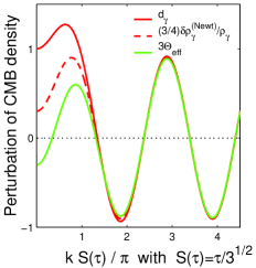
Figure 1: The evolution of a Fourier mode of CMB density perturbation in the radiation era in terms of different measures: Coordinate number density perturbation $d_{\gamma}=\delta n_{\gamma\,{\rm coo}}/n_{\gamma\,{\rm coo}}$ (solid), proper density perturbation $\delta\rho_{\gamma}/\rho_{\gamma}$ in the Newtonian gauge (dashed), and effective temperature perturbation $\Theta_{\rm eff}$, eq. (48), (green solid), all normalized to coincide on small scales.

However, in the concordance cosmological model as much as $41\%$ of the energy density in the radiation era is carried by decoupled neutrinos. The evolution of free-streaming neutrinos and their contribution to metric inhomogeneities differs qualitatively S. Bashinsky, U. Seljak (2004) from the acoustic dynamics of the photon fluid. If without neutrinos the CMB perturbations were resonantly boosted by metric inhomogeneities, neutrinos should be expected to significantly untune the “resonance”. In reality, neutrinos decrease subhorizon $\delta T/T$ by as little as $10\%$, as compared to subhorizon $\delta T/T$ in a model with identical inflation-generated primordial perturbations but no neutrinos. Moreover, the addition of noticeable density of early tracking quintessence Ratra and Peebles (1988); P. Ferreira, M. Joyce (1997); Zlatev et al. (1999); Ott (2001), whose perturbations evolve very dissimilar to the acoustic CMB perturbations (dashed vs solid lines in Fig. 2), not only fails to destroy the “resonance” but instead enhances subhorizon $\delta T/T$ (Fig. 3 a).

We argue that the apparent radiation driving of photon temperature in the Newtonian gauge is a gauge artifact. First, the driving is absent when CMB density perturbations are quantified by the measure $d_{\gamma}$, satisfying conditions I and II. Indeed, in a photon-dominated universe the overdensity $d_{\gamma}$ in the Newtonian gauge evolves as S. Bashinsky, U. Seljak (2004)

$$d_{\gamma}=d_{\rm in}\left(\frac{2\sin\varphi}{\varphi}-\cos\varphi\right),\quad\varphi\equiv k\tau/\sqrt{3},$$ (50)

as follows from eqs. (72) and (36). Hence, without neutrinos or early quintessence, the amplitude of subhorizon oscillations of photon overdensity, ${\rm Amp}[d_{\gamma}]$, exactly equals the primordial photon overdensity, $d_{\gamma}(\tau\to 0)=d_{\rm in}$. By Sec. II.4, any other measure of photon perturbations $d^{\prime}_{\gamma}$ that satisfies conditions I and II coincides with $d_{\gamma}$ on super- and subhorizon scales. Any such measure, therefore, would also detect no radiation driving: ${\rm Amp}[d_{\gamma}^{\prime}]=d_{\gamma}^{\prime}(\tau\to 0)$.

A formalism-independent distinction between physical driving of perturbations and a gauge artifact can be made by comparing the studied model to a reference model in which the metric becomes homogeneous by reentry. In the latter model any driving by metric inhomogeneities at reentry is objectively absent. A consistent procedure to achieve homogeneous geometry before reentry for any given primordial perturbations of arbitrary species was described in Sec. II.4. In the homogeneous (FRW) metric the evolution of photon fluid overdensity readily follows from eq. (73) with $c_{s}^{2}=1/3$ as

$$d_{\gamma}^{({\rm undriven})}=d_{\rm in}\cos\varphi.$$ (51)

Thus if in the superhorizon limit the photon and metric perturbations in the photon-dominated and “undriven” models are identical, after horizon entry the acoustic oscillations in the two models have equal amplitude. There is no causal mechanism for a gravitational boost of the amplitude in the second model. Therefore, the amplitude should also not be considered boosted in the photon-dominated model.

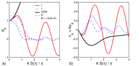
Figure 2: a) Density perturbations $d_{a}$ of typical cosmological species in the radiation epoch dominated by tightly coupled photons ($\gamma$, red solid) and 3 flavors of decoupled relativistic neutrinos ($\nu$, dash-dotted). The subdominant species are cold dark matter (CDM, black solid), and a scalar field (tracking quintessence $Q$, dashed). The primordial perturbations are assumed adiabatic. The dotted curve shows the equilibrium value of $d_{\gamma}$ oscillations, eq. (44). b) Bulk peculiar velocities of the same species.

The 3-fold increase of the Newtonian-gauge perturbation $\delta T_{\gamma}^{(\rm Newt)}\!/T_{\gamma}=\frac{1}{3}\,d_{\gamma}+\Psi$ in the second of the above models occurs when the metric becomes homogeneous on superhorizon scales. This increase can hardly be attributed to a resonant boost of the acoustic oscillations from the decay of their gravitational potential at the maximum photon compression, as stated in Hu and Dodelson (2002). The enhancement of the perturbation measure $\delta T_{\gamma}^{(\rm Newt)}\!/T_{\gamma}$ is possible because its evolution is not determined only by local dynamics.

V.2.2 Gravitational impact of perturbations on the CMB and CDM

Fig. 2 a) displays the linear evolution of coordinate density perturbations $d_{a}(\tau,k)$ in a photon-baryon fluid, decoupled relativistic neutrinos, CDM, and a minimally coupled scalar field [tracking quintessence, $Q$, with $w_{Q}(z)=w_{\rm total}(z)$]. Fig. 2 b) shows the corresponding bulk velocities of the species. The plots describe the radiation epoch, dominated by photons and three standard flavors of neutrino. They are obtained by the numerical integration of eqs. (60)-(101) and (36)-(37) with the regular adiabatic initial conditions, normalized to $d(k/{\cal H}\rightarrow 0)=1$. The chosen evolution parameter is a dimensionless phase of photon acoustic oscillations $kS(\tau)$ where $S(\tau)\equiv\int_{0}^{\tau}c_{s}d\tau=\tau/\sqrt{3}$ (for $R_{b}\ll 1$) is the size of the acoustic horizon.

In the description of the acoustic dynamics of the CMB by eq. (43), the gravitational impact of the species’ perturbations is mediated through the “restoring force” $-c_{s}^{2}k^{2}(d_{\gamma}-B)$, with

$$B(\tau,k)=\mbox{$-3(\Phi+\Psi+R_{b}\Phi)$}.$$ (52)

The potentials $\Phi$ and $\Psi$ are sourced by perturbations of densities, peculiar velocities, and anisotropic stress of the species as described by eqs. (36)-(37).

For typical cosmological species, the growth of subhorizon perturbations during the radiation era is insufficient for supporting a non-vanishing gravitational potential. Hence, the equilibrium photon overdensity $B(\tau,k)$ on subhorizon scales tends to zero. Thus in the radiation era the gravitational impact of perturbations is confined to horizon entry. As for the later subhorizon CMB oscillations, this impact can only rescale the oscillations’ amplitude and additively shift the phase. We now consider the gravitational impact on the CMB that is caused by decoupled relativistic neutrinos and a scalar field (early quintessence).

Addition of extra ultrarelativistic neutrinos changes $B$ as shown by the solid curve in Fig. 3 c). The increase of $N_{\nu}$ reduces $B$ during the initial growth of $d_{\gamma}$ while enhances $B$ for a significant period of $d_{\gamma}$ fall. The resulting modulation of the restoring force $-c_{s}^{2}k^{2}(d_{\gamma}-B)$ somewhat damps $d_{\gamma}$ oscillation. The reduction of the amplitude of CMB oscillations by neutrino perturbations Hu and Sugiyama (1996); S. Bashinsky, U. Seljak (2004) is evident from the thin solid curve in Fig. 3 a).

On the contrary, the density perturbation of canonical tracking quintessence Ratra and Peebles (1988); P. Ferreira, M. Joyce (1997); Zlatev et al. (1999); Ott (2001) is significantly reduced right after horizon entry [see the dashed line in Fig. 3 a).] This reduction causes a prominent drop in $B(\tau)$, shown by the dashed curve in Fig. 3 c), at the time when $\dot{d}_{a}$ is on average negative. As a result, the acoustic oscillations gain energy and their amplitude increases Ferreira and Joyce (1998).

The qualitative difference in the evolution of density perturbations for quintessence versus the other considered species can be understood as follows. For the regular adiabatic initial conditions, the number density perturbations $d_{a}$ of all the species are equal and the velocities vanish beyond the horizon ($kS\ll 1$). Moreover, the initial accelerations of all the species, eq. (42), are also equal, as confirmed by Fig. 2 b). However, the rate of change of $d_{a}$ at reentry is very sensitive to whether or not pressure of the species is fully specified by their local density. If it is, such as for photons, CDM, and neutrinos, the “nonadiabatic” term on the right-hand side of eq. (19) vanishes. The corresponding $d_{a}$’s agree in their evolution up to $O(k^{4}\tau^{4})$ corrections. On the other hand, for a classical field the nonadiabatic term becomes non-zero during the entry [c.f. the first of eqs. (101).] As a consequence, quintessence density perturbation $d_{Q}$ [dashed line in Fig. 2 a)] noticeably deviates from the perturbations of the other species already in $O(k^{2}\tau^{2})$ order.

Quantitatively, a change of $N_{\nu}$ from $3$ to $4$ changes the amplitude of $d_{\gamma}$ oscillations by $-1.7\%$. Addition of equal energy in the form of tracking quintessence, on the contrary, enhances the amplitude by $1.6\%$.

Perturbations of CDM evolve according to eqs. (60) as

$$d_{c}=-\int(\nabla_{\!i}v^{i}_{c})\,d\tau,\qquad av^{i}_{c}=-\int(a\nabla_{\!i}\Phi)\,d\tau.$$ (53)

The impact of metric perturbations on CDM is thus determined by a normalized quantity $-(a/a_{\rm ent})\Phi$, where $a_{\rm ent}\equiv a|_{k\tau=1}$. Fig. 3 d) shows how this quantity is affected by the addition of extra neutrinos and quintessence. By comparing Fig. 3 b) and Fig. 3 a), we see that the signs of the gravitational impact of perturbations in either neutrinos Hu and Sugiyama (1996); S. Bashinsky, U. Seljak (2004) or quintessence Caldwell et al. (2003) on the power of CDM are opposite to the signs of the impact of these species on the acoustic amplitude of the CMB. Thus on the scales entering the horizon before matter-radiation equality ($\ell\gtrsim 200$, $k\gtrsim 10^{-2}$ Mpc^-1) the ratio of CMB to CDM powers, which is insensitive to the unknown primordial power of cosmological perturbations, is slightly decreased by decoupled particles. On the other hand, this ratio is increased by tracking quintessence.

The gravitational impact of perturbations on the phase of CMB oscillations is easier to analyze in real space Magueijo (1992); Baccigalupi (1999); Bashinsky and Bertschinger (2001, 2002). The phase shift, along with all the other characteristics of subhorizon oscillations, is fully specified by the singularity of the CMB Green’s function at the acoustic horizon S. Bashinsky, U. Seljak (2004). An analysis of this singularity S. Bashinsky, U. Seljak (2004) shows that for adiabatic initial conditions the phase is affected only by the perturbations which propagate faster than the acoustic speed of the photon fluid.

Perturbations of both ultrarelativistic neutrinos and quintessence propagate at the speed of light $c$, i.e., faster than the acoustic speed $c_{s}\leq c/\sqrt{3}$. The phase shift induced by neutrinos displaces all the CMB peaks in the temperature and E-polarization spectra by an about equal multipole number S. Bashinsky, U. Seljak (2004)

$$\Delta l_{\nu}\approx-57\,\frac{\rho_{\nu}}{\rho_{\gamma}+\rho_{\nu}}.$$ (54)

The three standard types of neutrino give $\Delta l_{3\nu}\approx-23$, large enough to be observable with the present data Crotty et al. (2003b); Pierpaoli (2003); Hannestad (2003); Barger et al. (2003); Trotta and Melchiorri (2005); Bell et al. (2005); Spergel et al. (2006). One additional fully populated type of relativistic neutrino increases the shift by S. Bashinsky, U. Seljak (2004) $\Delta l_{+\nu}\simeq-3.4$. According to numerical integration of eqs. (60)-(101) and (36)-(37), the same additional radiation density ($\Delta N_{\rm eff}=+1$) in tracking quintessence leads to an almost triple shift $\Delta l_{Q}\simeq-11$.

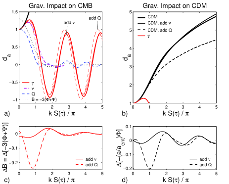
Figure 3: RADIATION ERA. The impact of perturbations in decoupled neutrinos and quintessence on the CMB and CDM. The wide solid curves give $d_{\gamma}$ (a) and $d_{\rm CDM}$ (b) in the epoch dominated by tightly coupled photons and three standard flavors of decoupled neutrinos. The thin solid curves describe a model with doubled neutrino energy density. The dashed curves describe a model with the standard neutrino content plus the same energy density in tracking quintessence, with $w_{Q}=1/3$. The bottom panels demonstrate how these modifications of the fiducial model change the gravitational terms which drive the CMB (c) and CDM (d).

While in a formal treatment of Boltzmann hierarchy for the perturbations of free-streaming neutrinos, e.g. Hannestad (2005), the anisotropic stress might appear to be the primary cause of their characteristic gravitational imprints, this conclusion is misleading. For example, anisotropic stress of minimally coupled tracking quintessence, whose perturbations also change the amplitude and phase of acoustic oscillations, is identically zero. In particular, a real space approach S. Bashinsky, U. Seljak (2004) shows that for adiabatic perturbations the phase is shifted if and only if some perturbations physically propagate faster than the acoustic speed $c_{s}$.

V.3 Matter era

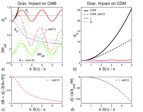
Figure 4: MATTER ERA. The perturbations of the CMB density $d_{\gamma}$ and effective temperature $\Theta_{\rm eff}$ (a) and of CDM density $d_{c}$ (b) in the matter era dominated by pressureless matter (solid curves) and by equal densities of pressureless matter and tracking quintessence, with $w_{Q}=0$ (dashed curves). Similarly to Fig. 3, the bottom panels show the change induced by quintessence in the gravitational terms which drive the CMB (c) and CDM (d).

V.3.1 25-fold Sachs-Wolfe suppression

In the epoch dominated by pressureless CDM and baryons which have decoupled from the CMB, metric perturbations (gravitational potentials) do not decay on subhorizon scales. Through the finite potentials, matter continues to influence CMB long after horizon entry. For the perturbations entering the horizon in this epoch, matter overdensity grows linearly in the scale factor $a\propto\tau^{2}$, as $d=d_{\rm in}(1+k^{2}\tau^{2}/30)$. If the initial conditions are adiabatic, photon and neutrino perturbations contribute negligibly to inhomogeneities of the metric in the matter era. Then Newtonian gravitational potentials, induced entirely by perturbations of nonrelativistic matter, remain time-independent throughout all the linear evolution:

$$\Phi=\Psi=-\frac{1}{5}\,d_{\rm in},$$ (55)

as can be verified with eqs. (36) and (60).

The acoustic dynamics and subsequent free-streaming of CMB photons in the gravitational wells of non-relativistic matter are well understood on subhorizon scales, e.g. Bond and Efstathiou (1987); Hu and Sugiyama (1996); Hu et al. (1997); Hu and Dodelson (2002); Dodelson (2003); Mukhanov (2005). However, the traditional description of horizon entry in the matter era, e.g. Hu and Sugiyama (1995b, a); Hu et al. (1997); Hu and Dodelson (2002), requires corrections.

For the considered perturbations, entering the horizon after CMB last scattering but long before dark energy domination, the Doppler and polarization contributions to the observed CMB anisotropy $\Delta T/T$ [second and third terms in eq. (49)] are negligible. The ISW contribution $\dot{\Phi}+\dot{\Psi}$ is also absent. Indeed, the potentials are static during the matter era and their later decay due to the dark energy domination is for these modes adiabatically slow. The remaining contribution to the observed $\Delta T/T$ (49) is then described by the effective temperature perturbation $\Theta_{\rm eff}$ (48),

$${\Delta T\over T}=\Theta_{\rm eff}=\left.{\delta T\over T}\right|_{\rm in}+2\Phi.$$ (56)

Here, we defined

$$\left.{\delta T\over T}\right|_{\rm in}\equiv\frac{1}{3}\,d_{\gamma,\,\rm in},$$ (57)

with $d_{\gamma,\,\rm in}\equiv d_{\gamma}(k\ll{\cal H}(\tau))$ and set $\Phi=\Psi$ in the matter era. The quantity (57) is a natural measure of the intrinsic CMB temperature perturbation on superhorizon scales. This is the perturbation to be always observed for the decoupled CMB photons if the metric becomes homogeneous on superhorizon scales and remains such during the subsequent evolution.

If the initial conditions are adiabatic (Sachs-Wolfe case) then, by eq. (55), $\Phi=-\frac{1}{5}d_{\rm in}=-\frac{1}{5}d_{\gamma,\,\rm in}$. Thus the classical Sachs-Wolfe result $\Delta T/T=\Phi/3$ R. K. Sachs, A. M. Wolfe (1967) is due to a partial cancellation of the primordial CMB density perturbation $\left.{\delta T/T}\right|_{\rm in}=-\frac{5}{3}\,\Phi$ against the gravitational redshift $2\Phi$ in proportion $-5:6$. The 5-fold suppression of the primordial temperature perturbation results in an astonishing (and experimentally evident) suppression of the angular power of CMB temperature $C_{l}$ by a factor of $25$.

The traditional interpretations of the Sachs-Wolfe result also note certain, 2-fold rather than 5-fold, suppression of the intrinsic CMB temperature fluctuations by the matter potential. The relation $\Delta T/T=\Phi/3$ is usually interpreted as a partial cancellation between the “intrinsic” temperature anisotropy $\delta T^{\rm(Newt)}/T|_{\rm in}=-\frac{2}{3}\Phi$ and the gravitational redshift $\Phi$ Hu and Sugiyama (1995b, a); Hu et al. (1997); Hu and Dodelson (2002):

$$\qquad\qquad{\Delta T\over T}=\left.{\delta T^{\rm(Newt)}\over T}\right|_{\rm in}\!\!+\Phi\quad(\rm misleading!)$$ (58)

Let us present two examples where such quasi-Newtonian considerations lead to wrong expectations.

One example is a classical scenario of “isocurvature” initial conditions, e.g., from a phase transition early in the radiation era, when $\rho_{\gamma}\gg\rho_{c}$. If immediately after the phase transition $\delta\rho_{\gamma}+\delta\rho_{c}=0$ then $|\delta\rho_{\gamma}/\rho_{\gamma}|\ll|\delta\rho_{c}/\rho_{c}|$. For a fixed magnitude of cosmological inhomogeneities $|\delta\rho_{c}/\rho_{c}|\sim 10^{-5}$, the primordial photon perturbations $\delta\rho_{\gamma}/\rho_{\gamma}$ can then be ignored. However, it would be wrong to conclude that $\delta T^{\rm(Newt)}/T|_{\rm in}=0$ and that from eq. (58), due to the gravitational redshift in the matter era, $\left.{\Delta T/T}\right|_{\rm isoc}=\Phi$ (incorrect!). The correct answer is $\left.{\Delta T/T}\right|_{\rm isoc}=2\Phi$, in agreement with eq. (56) where now $\left.{\delta T/T}\right|_{\rm in}=0$.

Another example where the interpretation (58) misleads is the opposite case of non-zero $\delta\rho_{\gamma}/\rho_{\gamma}$ but homogeneous and isotropic geometry in the matter era. If the primordial perturbations of radiation in this scenario are identical to the perturbations in the adiabatic model then the interpretation (58) suggests that now, when the “2-fold” suppression by $\Phi$ is absent, $\left.{\Delta T/T}\right|_{\Phi=0}=-2\left.{\Delta T/T}\right|_{\rm adiab}$ (incorrect!). The correct answer, immediate from eqs. (56) and (57), is

$$\left.{\Delta T\over T}\right|_{\Phi=0}=\left.{\delta T\over T}\right|_{\rm in}=-5\left.{\Delta T\over T}\right|_{\rm adiab},$$ (59)

in agreement with our claim of 5-fold suppression of $\Delta T/T$ by $\Phi$ in the adiabatic case.

The homogeneous geometry of the last scenario could be generated with the matter initial conditions $d_{m,\,\rm in}\approx 0$, yet there is no physical reason to expect such initial conditions Linde et al. (2005). However, $d_{c}$ and the matter-induced potentials $\Phi$ and $\Psi$ may be partly smoothed early during the horizon entry by non-standard dynamics of the dark sector. In the limiting case of a perfectly homogeneous metric since very early time, we recover the unsuppressed CMB oscillations, with the amplitude $d_{\gamma,\,\rm in}$ in overdensity and $\Delta T/T=\left.{\delta T/T}\right|_{\rm in}=-5\left.{\Delta T/T}\right|_{\rm adiab}$ in temperature.

V.3.2 Implications

The observed CMB multipoles with $\ell\lesssim 200$ are primarily generated by the perturbation modes which enter the horizon during the matter era. These modes evolve in a static potential of collapsing CDM and baryons. The potential suppresses the corresponding $C_{l}$’s by an order of magnitude, see the solid curve in Fig. 5 for the “concordance” $\Lambda$CDM model Spergel et al. (2003); Tegmark et al. (2004); Seljak et al. (2005); Spergel et al. (2006).

The suppression is somewhat reduced for $\ell\lesssim 10$ because of the modes which enter the horizon when dark energy becomes dominant and the potential decays. For these modes the enhancement of CMB power is fully described by the ISW term $\dot{\Phi}+\dot{\Psi}$, eq. (49). In general, however, the reduction of the 25-fold Sachs-Wolfe suppression is not equivalent to the ISW enhancement. An extreme example is the scenario in which $\Phi+\Psi$ vanishes prior to CMB decoupling. Given equal primordial perturbations, the observed CMB power $C_{l}$ in this scenario exceeds the Sachs-Wolfe power by 25 times, although in both scenarios the ISW effect is absent.

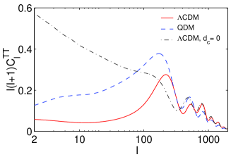
Figure 5: Suppression of the angular power spectrum of CMB temperature $C_{l}$ for $\ell\lesssim 200$ by dark matter perturbations. The figure compares three models which differ only by perturbations in the dark sector: The “concordance” $\Lambda$CDM model Spergel et al. (2003); Tegmark et al. (2004); Seljak et al. (2005); Spergel et al. (2006) (solid); a model where CDM and cosmological constant are replaced by a dynamical scalar field with the same background $\rho(z)$ (dashed, the overall power of perturbations is decreased to match the concordance $C_{300}$); finally, a $\Lambda$CDM model where CDM density is artificially arranged to be unperturbed beyond the horizon (dash-dotted, the primordial power of photon, baryon, and neutrino perturbations is the same as in the concordance model).

More realistically, the density perturbation $d_{a}$ of some of the dominant species in the matter era may grow slower than $[a^{2}(\rho+p)]^{-1}\sim 1/{\cal H}^{2}\sim\tau^{2}$. Then, by eq. (36), these species contribute only decaying terms to the gravitational potentials. This diminishes the suppression of the CMB power at $\ell\lesssim 200$. As an illustration, the upper solid and dashed curves in Fig. 4 a) show $d_{\gamma}$ in a CDM-dominated universe (Sachs-Wolfe case) and in a model where the energy density of the dark sector is split equally between CDM and quintessence whose background density tracks CDM. In the second model the CMB temperature perturbations on subhorizon scales are larger by $93\%$.

Thus any physics which reduces metric inhomogeneities in the matter era strongly influences CMB temperature anisotropy. Some of the influence may be due to a different ISW effect from the temporal change of the gravitational potentials. It can also be due to reduced gravitational lensing of the CMB, appearing in the second perturbative order. However, the most prominent impact is caused by the very reduction of the potentials, suppressing the auto-correlation of CMB temperature by a factor of 25.

Two examples are shown in Fig. 5. The figure displays the CMB temperature power spectra $C_{l}$ obtained with a modified cmbfast code Seljak and Zaldarriaga (1996) for three models which differ only by the dynamics of perturbations in the dark sectors. The solid curve describes the concordance $\Lambda$CDM model Spergel et al. (2003); Tegmark et al. (2004); Seljak et al. (2005); Spergel et al. (2006). The dashed curve refers to a model where the dark sector is composed entirely of a classical canonical scalar field $Q$. In this model at every redshift the field background density $\rho_{Q}(z)$ is chosen to equal the combined CDM and vacuum densities $\rho_{c}(z)+\rho_{\Lambda}$ of the $\Lambda$CDM model. However, since the field perturbations do not grow, the metric inhomogeneities of the second model decay after the horizon entry in the matter era. As a result, its CMB power for $\ell\lesssim 200$ is enhanced.

The last, dash-dotted, curve in Fig. 5 describes a model which has the matter content of the concordance $\Lambda$CDM model. However, while in the previous two scenarios the initial conditions were adiabatic, here CDM density perturbation $d_{c}$ is set to zero on superhorizon scales (the initial values for $d_{\gamma}$, $d_{\nu}$, and $d_{b}$ are unchanged). Then, again, the metric inhomogeneities in the matter era are reduced. While this model has the least ISW effect, the smoother metric causes the largest enhancement of the CMB power among the compared models for $\ell\lesssim 200$.

VI Summary

There is a variety of descriptions of inhomogeneous cosmological evolution which are apparently dissimilar on the scales exceeding the Hubble scale. To single out the descriptions least afflicted by gauge artifacts, we suggest considering the measures of perturbations that meet the following criteria: I. The measure’s dynamics is determined entirely by the physics within the local Hubble volume. II. The measure is practically applicable in Minkowski limit and retains its physical meaning in any FRW geometry on all scales.

We showed (Sec. II.1) that in the fully nonlinear theory these criteria are fulfilled for a perturbation of one-particle phase-space distribution $f(x^{\mu},P_{i})$, considered as a function of particle canonical momenta $P_{i}$. The often used perturbations of $f(x^{\mu},{\bm{p}})$ or $f(x^{\mu},{\bm{q}})$, where ${\bm{p}}$ is the proper momentum and ${\bm{q}}\equiv a{\bm{p}}$, do not satisfy requirement I. Perturbed nonlinear dynamics of radiation can be appropriately described by the intensity perturbation $\iota(x^{\mu},n_{i})$, constructed by integration of $f(x^{\mu},P_{i})$, eqs. (7) and (9). Finally, a description of perturbed linear dynamics of arbitrary species satisfies criteria I and II if the perturbations are quantified by coordinate number density perturbations $d=\delta n_{{\rm coo}}/n_{{\rm coo}}$, eq. (20). In linear theory these measures of perturbations in phase-space distribution, intensity, and density are interrelated with eqs. (24) and (25).

Similarly to the traditional proper measures of perturbations, e.g. $\Delta T(\hat{\bf n})/T$ and $\delta\rho/\rho$, the proposed ”coordinate” measures $\iota(n_{i})$ and $d=\delta n_{{\rm coo}}/n_{{\rm coo}}$ are gauge-dependent. Yet the gauge dependence of the proposed, but not traditional, measures disappears in the superhorizon limit. More generally, we prove that on superhorizon scales the values of the density perturbations are the same in terms of any measure satisfying the formal versions of criteria I and II, namely, conditions I^′ and II^′ on page I^′..

In the Newtonian gauge (26) the suggested variables provide additional technical advantages. One is the explicit Cauchy structure of the dynamical equations (eq. (19), Sec. III.2, and Appendix A). Another is a nonsingular superhorizon limit of the generalized gravitational Poisson equation (Sec. III.3). Analytical solutions in the new formulation inevitably appear more tractable S. Bashinsky, U. Seljak (2004). As an example, compare the solutions for density perturbations in the photon-dominated model, eq. (50) versus the traditional solution in Footnote 10.

In the proposed class of formalisms, classical linear density perturbations of individual species manifestly decouple gravitationally on superhorizon scales. This view of linear superhorizon evolution of multiple species (Sec. IV.1) agrees with the picture provided by the conserved curvatures of Wands et al. Wands et al. (2000). The density perturbations of the species recouple during the horizon entry (Sec. IV.2).

On the other hand, our description reveals a different from the traditionally assumed origin of several prominent features in the angular power of CMB temperature $C_{\ell}$. First of all, the apparent “resonant boost” of CMB perturbations for $\ell\gtrsim 200$, presumably by their self-gravity during the horizon entry in the radiation era Hu and Sugiyama (1996); Hu et al. (1997, 2001); Hu and Dodelson (2002); Dodelson (2003); Mukhanov (2005), is found to be a gauge artifact of the Newtonian gauge. We demonstrated (Sec.V.2.1) that the driving is absent when density perturbations are quantified by any measure satisfying conditions I^′ and II^′.

We showed (Sec. V.2.1) that the “radiation driving” picture leads to incorrect expectations for the observed CMB signatures of dark species. Since the resonant self-boost of CMB perturbations does not physically exist and cannot be untuned by the gravitational influence of non-photon species present in the radiation era with non-negligible densities, the CMB signatures of such species are not anomalously amplified. This corrected expectation is confirmed by calculations for decoupled relativistic neutrinos and for tracking quintessence (Ref. S. Bashinsky, U. Seljak (2004) and Sec. V.2.2).

A moderate impact of such species on the CMB power at small scales, less affected by cosmic variance, nevertheless already allows meaningful constraints on the species’ abundance and nature, Refs. Crotty et al. (2003b); Pierpaoli (2003); Hannestad (2003); Barger et al. (2003); Spergel et al. (2006); Hannestad (2005); Trotta and Melchiorri (2005); Bell et al. (2005). The constraints will significantly improve in the near future Lopez et al. (1999); Bowen et al. (2002); S. Bashinsky, U. Seljak (2004), when the smaller angular scales become resolved.

Notably, the CMB is sensitive to the propagation velocity of small-scale inhomogeneities in the dark sectors J. K. Erickson et al. (2002). For neutrinos, quintessence, and any other species for which this velocity exceeds the sound speed in the photon fluid $c_{s}\approx c/\sqrt{3}$, the perturbations cause a nondegenerate uniform shift of the acoustic peaks S. Bashinsky, U. Seljak (2004); Bashinsky (2004). The CMB power is also sensitive to nonadiabatic pressure, generally developing for a classical field. As discussed in Sec. V.2.2, under adiabatic initial conditions, the nonadiabatic pressure affects the evolution of species’ overdensities already at the order $O(k^{2}\tau^{2})$ while the regular pressure enters only at $O(k^{4}\tau^{4})$. In the example of tracking quintessence, nonadiabatic pressure causes early suppression of quintessence density perturbations (Sec. V.2.2 and Fig. 2). This enhances the CMB power while neutrino perturbations reduce it (Fig. 3).

Although CMB perturbations are not resonantly boosted on small scales, the CMB multipoles with $\ell\lesssim 200$ are significantly suppressed by the gravitational potential which does not decay after the horizon entry in the matter era. The contribution of the perturbations which enter the horizon when $|\delta p/\delta\rho|\ll 1$ and the potential is time-independent, to the angular power of CMB temperature is suppressed by 25 times (Sec. V.3.1). The suppression is thus much more prominent than a factor of 4 reduction of the CMB power in the conventional interpretations Hu and Sugiyama (1995b, a); Hu et al. (1997); Hu and Dodelson (2002) of the Sachs-Wolfe effect R. K. Sachs, A. M. Wolfe (1967).

As a consequence, any mechanism which smoothes metric inhomogeneity after radiation-matter equality at redshift $z\sim 3500$ significantly enhances CMB anisotropy (Sec. V.3.2). Examples of such mechanisms are a noticeable fraction of quintessence at all post-equality redshifts, interaction or unification of dark matter and dark energy, e.g. Wetterich (1988); Perrotta and Baccigalupi (2002); G. R. Farrar, P. J. Peebles (2004); Catena et al. (2004); Scherrer (2004), or alternative explanations for the apparent signatures of nonbaryonic matter, e.g. MOND-inspired theory of gravity Bekenstein (2004). The enhancement is accounted for by the ISW effect when the metric is smoothed after CMB last scattering at $z\sim 1100$. However, even if the ISW effect is absent, but the metric at or before CMB last scattering is already smoother than in the standard scenario, the enhancement exists. Thus the experimentally evident suppression of CMB multipoles with $\ell\lesssim 200$ severely constrains the mechanisms which reduce metric perturbations at any time in the matter era.

Appendix A Perturbative Dynamics of Typical Species

In this Appendix we give the closed equations for the linear evolution of scalar perturbations of typical cosmological species: cold dark matter ($c$), decoupled neutrinos ($\nu$), photon-baryon plasma ($\gamma b$), and a classical scalar field, or quintessence, ($\varphi$). We use the Newtonian gauge (26), in which the gravitational potentials $\Phi$ and $\Psi$ are determined by the perturbations of the total density, velocity, and anisotropic stress with eqs. (36)-(37).

A.1 Cold dark matter (CDM)

Before CDM streams cross, in particular, in the linear regime, CDM is equivalent to a fluid with vanishing pressure and vanishing anisotropic stress ($p_{c}=\delta p_{c}=0$, $\sigma_{c}=0$). Then from eqs. (19) and (31)

$$\dot{d}_{c}=\nabla^{2}u_{c},\qquad\dot{u}_{c}=-{\cal H}u_{c}+\Phi.$$ (60)

Elimination of $u_{c}$ gives a single second-order equation for CDM density perturbation

$$\textstyle\ddot{d}_{c}+{\cal H}\dot{d}_{c}=\nabla^{2}\Phi.$$ (61)

A.2 Neutrinos

A.2.1 General case

When the universe cools below $1$ MeV, weak interactions of the standard neutrinos become cosmologically irrelevant. Then the full evolution of neutrino phase-space distribution $f$ is governed by collisionless Boltzmann equation (2). Straightforward linearization of eq. (2) shows that the scalar component of $f$ perturbation

$$df(x^{i},P_{i})\equiv f(x^{i},P_{i})-\bar{f}(P)$$ (62)

evolves in the linear order in the Newtonian gauge (26) as

$$\left(df\right)^{\!\displaystyle\cdot}+V_{i}\,\nabla_{\!i}\left(df\right)=E\,\frac{\,\partial\!\bar{f}}{\partial E}\,V_{i}\,\nabla_{\!i}\left(\Phi+V^{2}\,\Psi\right),$$ (63)

where $E\equiv(P^{2}+m^{2}a^{2})^{1/2}$ and $V_{i}\equiv P_{i}/E$.

The initial conditions for the perturbation $df$ on superhorizon scales can be determined as follows. Consider spatial hypersurfaces of constant radiation density $\rho_{r}$ and, to be specific, assume that neutrino chemical potential is unperturbed. Then prior to neutrino decoupling the neutrino phase-space distribution $f_{\rm pr}(\bm{p}_{\rm pr})$ in proper variables $d^{3}{\bm{x}}_{\rm pr}d^{3}\bm{p}_{\rm pr}$ is spatially uniform (independent of $x^{i}$) on a hypersurface $\rho_{r}={\rm const}$. In a gauge of uniform radiation density and zero shear, in which $\rho_{r}={\rm const}$ defines the hypersurfaces of constant time and the 3-metric is $g_{ij}=a^{2}(1+2\zeta_{r})\delta_{ij}$, the proper and canonical neutrino momenta are related as $p^{i}_{\rm pr}=P_{i}/[a(1+\zeta_{r})]$. Thus in the variables $(x^{i},P_{i})$

$$f(x^{i},P_{i})=f_{\rm pr}\left(\frac{P_{i}}{a[1+\zeta_{r}(x^{i})]}\right).$$ (64)

(We used that $d^{3}{\bm{x}}_{\rm pr}d^{3}\bm{p}_{\rm pr}=d^{3}x^{i}d^{3}P_{i}$.) The corresponding linear perturbation of $f(x^{i},P_{i})$ is

$$df=-P\frac{\partial\bar{f}(P)}{\partial P}\,\zeta_{r}(x^{i}).$$ (65)

Note that substitution of the last result in eq. (24) or integration of eq. (64) over $d^{3}P_{i}$ returns $d_{\nu}=3\zeta_{r}$.

Since $f(x^{i},P_{i})$ is a 4-scalar and for the decoupled particles $\bar{f}(P)$ is time-independent, $df$ is a gauge invariant. Therefore, eq. (65) gives the initial conditions for $df$ evolution in any gauge, including the Newtonian.

A.2.2 Ultrarelativistic limit

Perturbation of the intensity of ultrarelativistic neutrinos is conveniently described by the variable $\iota(x^{\mu},n_{i})$, introduced by eq. (9). After neutrino decoupling, the full and the linear evolution of neutrino intensity perturbation is given by eqs. (10) and (15) respectively. The latter shows that for linear scalar modes in the Newtonian gauge

$$\dot{\iota}_{\nu}+n_{i}\nabla_{\!i}\iota_{\nu}=-4n_{i}\nabla_{\!i}(\Phi+\Psi).$$ (66)

Scalar perturbations of $\iota_{\nu}(n_{i})$ may be parameterized by scalar multipole potentials $d_{\nu l}$ as S. Bashinsky, U. Seljak (2004)

$$\textstyle\frac{3}{4}\iota(n_{i}) \equiv D(n_{i})\,=$$ (67)

$$= \sum_{l=0}^{\infty}(-1)^{l}\,(2l+1)\,P_{l}\!\left(n_{i}\textstyle\frac{\nabla_{\!i}}{\nabla}\right)\nabla^{l}d_{l},$$

where $P_{l}(z)$ are the Legendre polynomials. The potentials $d_{\nu l}$ with $\ell=0,\,1$, and $2$ describe the neutrino number density perturbation, velocity potential, and anisotropic stress potential respectively: $d_{\nu 0}=d_{\nu}$, $d_{\nu 1}=u_{\nu}$, and $d_{\nu 2}=\sigma_{\nu}$ S. Bashinsky, U. Seljak (2004). In the special case of a plane-wave perturbation $\iota({\bm{x}})\propto\exp{(i{\bm{k}}\cdot{\bm{x}})}$, $\nabla^{l}d_{l}$ are proportional to the scalar ($m=0$) multipoles $\iota_{l0}=\int d^{2}\hat{\bf n}\,Y^{*}_{l0}(n_{i})\iota(n_{i})$, where the polar direction is taken along ${\bm{k}}$. By eq. (66) and the identity $(2l+1)\mu P_{l}(\mu)=(l+1)P_{l+1}(\mu)+lP_{l-1}(\mu)$, the neutrino multipole potentials evolve as

$$\textstyle\dot{d}_{\nu l}=\frac{l}{2l+1}\,d_{\nu,l-1}+\frac{l+1}{2l+1}\,\nabla^{2}d_{\nu,l+1}+\delta_{l1}(\Phi+\Psi)$$ (68)

($\delta_{l1}$ in the last term is the Kronecker symbol.)

A.3 Photon-baryon plasma

A.3.1 Tight coupling limit

Perturbations in the tightly coupled photon-baryon plasma ($u_{\gamma}=u_{b}$, $\sigma_{\gamma b}=0$) propagate as sound waves with an acoustic speed, e.g. Dodelson (2003),

$$c_{s}^{2}\equiv{\delta p_{\gamma b}\over\delta\rho_{\gamma b}}={\dot{p}_{\gamma b}\over\dot{\rho}_{\gamma b}}=\frac{1}{3(1+R_{b})}.$$ (69)

Here $R_{b}\equiv\rho_{b}/(\rho_{\gamma}+p_{\gamma})=3\rho_{b}/(4\rho_{\gamma})$ and the photon-baryon perturbations are assumed internally adiabatic ($d_{\gamma}=d_{b}$). In this limit, from eq. (19) and eqs. (31), (27),

$$\begin{array}[]{rcl}\dot{d}_{\gamma}&=&\nabla^{2}u_{\gamma},\\ \dot{u}_{\gamma}&=&c_{s}^{2}\,d_{\gamma}-{\cal H}(1-3c_{s}^{2})u_{\gamma}+\Phi+3c_{s}^{2}\Psi.\vphantom{\displaystyle{I\over I}}\end{array}$$ (72)

Elimination of $u_{\gamma}$ yields

$$\textstyle\ddot{d}_{\gamma}+{\cal H}(1-3c_{s}^{2})\,\dot{d}_{\gamma}-c_{s}^{2}\nabla^{2}d_{\gamma}=\nabla^{2}(\Phi+3c_{s}^{2}\Psi).~{}~{}~{}$$ (73)

To describe photon and baryon inhomogeneities beyond the tight coupling limit we should confront directional variation of photon intensity and account for the dependence of photon-baryon scattering on photon polarization.

A.3.2 Photon intensity

The scalar component of the perturbation $\iota_{\gamma}(n_{i})$ of polarization-summed photon intensity evolves according to the transport equation (33) with additional Thomson scattering terms Kaiser (1983); Bond and Efstathiou (1984); C.-P. Ma, E. Bertschinger (1995):

$$\dot{\iota}_{\gamma}\! + \!n_{i}\nabla_{\!i}\iota_{\gamma}=-4n_{i}\nabla_{\!i}(\Phi+\Psi)+$$

$$+ \!\frac{1}{\tau_{c}}\left\{-\iota_{\gamma}+\frac{4}{3}\,d_{\gamma}+4n_{i}v_{b}^{i}+\left[(n_{i}\nabla_{\!i})^{2}-\frac{1}{3}\nabla^{2}\right]\!\pi_{\!p}\right\}.$$

Here,

$$\tau_{c}\equiv({{an_{e}\sigma}}_{\!\rm Thomson})^{-1}$$ (75)

is a mean conformal time of a photon collisionless flight, $v_{b}^{i}=-\nabla_{\!i}u_{b}$ is the velocity of baryons, and $\pi_{\!p}$ is defined below by eq. (87). Similarly to the case of neutrinos, we introduce scalar multipoles $d_{\gamma l}$ of photon intensity perturbation $\iota_{\gamma}(n_{i})$ according to expansion (67). Then transport equation (A.3.2) expands into a hierarchy of multipole evolution

$$\begin{array}[]{rcl}\dot{d}_{\gamma}&=&\nabla^{2}u_{\gamma},\\ \dot{u}_{\gamma}&=&\frac{1}{3}\,d_{\gamma}+\frac{2}{3}\nabla^{2}\sigma_{\gamma}+\Phi+\Psi-\frac{1}{\tau_{c}}\left(u_{\gamma}-u_{b}\right),\vphantom{\displaystyle{\hat{I}\over\hat{I}}}\\ \dot{\sigma}_{\gamma}&=&\frac{2}{5}\,u_{\gamma}+\frac{3}{5}\,\nabla^{2}d_{\gamma,3}-\frac{1}{\tau_{c}}\left(\sigma_{\gamma}-\frac{1}{10}\,\pi_{\!p}\right),\vphantom{\displaystyle{I\over I}}\vphantom{\displaystyle{\hat{I}\over\hat{I}}}\\ \dot{d}_{\gamma l}&=&\frac{l}{2l+1}\,d_{\gamma,l-1}+\frac{l+1}{2l+1}\,\nabla^{2}d_{\gamma,l+1}-\frac{1}{\tau_{c}}\,d_{\gamma l},~{}~{}l\geq 3,\vphantom{\displaystyle{\hat{I}\over\hat{I}}}\end{array}$$ (80)

where for the last equation $d_{\gamma 2}=\sigma_{\gamma}$.

A.3.3 Photon polarization

The phase-space density of partially polarized photons with spacetime position $x^{\mu}$ and momentum $P_{i}$ is described by a $2\times 2$ Hermitian tensor $f_{\alpha\beta}(x^{\mu},P_{i})$, whose indexes $\alpha$ and $\beta$ refer to two spatial directions orthogonal to $P_{i}$. Given a polarimeter selecting the photons whose electric field varies as $\bm{E}\propto\hat{\bm{\epsilon}}\exp(iP_{i}x^{i})$, where $\hat{\bm{\epsilon}}$ is a complex unit 3-vector orthogonal to $P_{i}$ ($g_{ij}\epsilon^{*i}\epsilon^{j}=1$ and $P_{i}\epsilon^{i}=0$), the tensor $f_{\alpha\beta}$ specifies the phase-space density of the photons passing the polarimeter as $\epsilon^{*\alpha}f_{\alpha\beta}\epsilon^{\beta}$.

We define the intensity tensor of partially polarized photons by integrating $f_{\alpha\beta}(x^{\mu},P_{i})$ over $P^{3}dP$, similarly to eq. (7):

$$I_{\alpha\beta}(x^{\mu},n_{i})\equiv\int_{0}^{\infty}P^{3}dP\,f_{\alpha\beta}(x^{\mu},n_{i}P).$$ (81)

The connection of $I_{\alpha\beta}$ to the energy-momentum tensor of photons with a specific polarization $\hat{\bm{\epsilon}}$ is given by eq. (6) with $I\to\epsilon^{*\alpha}f_{\alpha\beta}\epsilon^{\beta}$. Finally, we generalize the intensity perturbation $\iota$ of eq. (9) to polarized radiation as

$$\iota_{\alpha\beta}(x^{\mu},n_{i})\equiv\frac{I_{\alpha\beta}}{\bar{I}}-1,$$ (82)

where $\bar{I}\equiv\mathop{\rm Tr}\bar{I}_{\alpha\beta}$ is the polarization-summed background intensity.

We will restrict the discussion of polarization evolution to harmonic plane-wave perturbations, which vary in space as $\exp{(i{\bm{k}}\cdot{\bm{x}})}$. While the general analysis is also possible, we defer it to a separate publication. In linear theory, solving the evolution of the plane-wave perturbations is sufficient for constructing the CMB transfer functions, summarized in Appendix B.

For the plane-wave perturbations of intensity $\iota_{\alpha\beta}(\hat{\bf n})$, we use the standard basis vectors $\hat{\bm{\epsilon}}_{\theta}$ and $\hat{\bm{\epsilon}}_{\phi}$, both orthogonal to $\hat{\bf n}$, where $\hat{\bm{\epsilon}}_{\theta}$ lies in the (${\bm{k}}$, $\hat{\bf n}$) plain and $\hat{\bm{\epsilon}}_{\phi}$ is orthogonal to it. In the basis $(\hat{\bm{\epsilon}}_{\theta},\hat{\bm{\epsilon}}_{\phi})$, a scalar (axially symmetric about ${\bm{k}}$) perturbation $\iota_{\alpha\beta}$ has the general form Basko and Polnarev (1980)

$$\iota_{\alpha\beta}=\frac{1}{2}\left(\begin{array}[]{cc}\iota+q&0\\ 0&\iota-q\end{array}\right).$$ (85)

Its Stokes’ polarization parameters are $Q=q(x^{\mu},\hat{\bm{k}}\,{\cdot}\,\hat{\bf n})$ and $V=U=0$.

The photon polarization $q_{\gamma}(x^{\mu},n_{i})$ evolves according to a transport equation Kaiser (1983); Bond and Efstathiou (1984); C.-P. Ma, E. Bertschinger (1995)

$$\dot{q}_{\gamma}+n_{i}\nabla_{\!i}q_{\gamma}=\frac{1}{\tau_{c}}\left\{-q_{\gamma}+[(n_{i}\nabla_{\!i})^{2}-\nabla^{2}]\pi_{\!p}\right\}\!.~{}~{}$$ (86)

In the last terms of eqs. (86) and (A.3.2),

$$\pi_{\!p}\equiv\sigma_{\gamma}+\tilde{p}_{\gamma 0}+p_{\gamma 2}.$$ (87)

The variables $\tilde{p}_{\gamma 0}$ and $p_{\gamma 2}$ are defined by the following expansion of $q_{\gamma}(n_{i})$ into scalar multipole potentials Bashinsky and Bertschinger (2002):

$$\textstyle\frac{3}{4}q_{\gamma}(n_{i}) = -\nabla^{2}\tilde{p}_{\gamma 0}+3(n_{i}\nabla_{\!i})\nabla^{2}\tilde{p}_{\gamma 1}\,+$$

$$+\ \sum_{l=2}^{\infty}(-1)^{l}\,(2l+1)\,P_{l}\!\left(n_{i}\textstyle\frac{\nabla_{\!i}}{\nabla}\right)\nabla^{l}p_{\gamma l}.$$

The hierarchy of evolution equations for the polarization multipole potentials follows from eq. (86) as

$$\begin{array}[]{rcl}\dot{\tilde{p}}_{\gamma 0}&=&\nabla^{2}\tilde{p}_{\gamma 1}-\frac{1}{\tau_{c}}\left(\tilde{p}_{\gamma 0}-\frac{1}{2}\,\pi_{\!p}\right),\vphantom{\displaystyle{\hat{I}\over\hat{I}}}\\ \dot{\tilde{p}}_{\gamma 1}&=&\frac{1}{3}\,\tilde{p}_{\gamma}{}_{0}-\frac{2}{3}\,p_{\gamma 2}-\frac{1}{\tau_{c}}\,\tilde{p}_{\gamma 1},\vphantom{\displaystyle{\hat{I}\over\hat{I}}}\\ \dot{p}_{\gamma 2}&=&-\frac{2}{5}\,\nabla^{2}\tilde{p}_{\gamma 1}+\frac{3}{5}\,\nabla^{2}p_{\gamma,3}-\frac{1}{\tau_{c}}\left(p_{\gamma 2}-\frac{1}{10}\,\pi_{\!p}\right),\vphantom{\displaystyle{\hat{I}\over\hat{I}}}\\ \dot{p}_{\gamma l}&=&\frac{l}{2l+1}\,p_{\gamma,l-1}+\frac{l+1}{2l+1}\,\nabla^{2}p_{\gamma,l+1}-\frac{1}{\tau_{c}}\,p_{\gamma l},~{}~{}l\geq 3.\vphantom{\displaystyle{\hat{I}\over\hat{I}}}\end{array}$$ (93)

A.3.4 Baryons

The evolution equations for baryons are similar to eq. (60) for CDM. The growth of the baryon density perturbation is, again, minus the divergence of their velocity. The equation for baryon acceleration contains all the terms of eq. (60) and an additional photon pressure term, related to the last term in $\dot{u}_{\gamma}$ equation (80) by local momentum conservation in photon-baryon scattering C.-P. Ma, E. Bertschinger (1995):

$$\begin{array}[]{rcl}\dot{d}_{b}&=&\nabla^{2}u_{b},\\ \dot{u}_{b}&=&-{\cal H}\,u_{b}+\Phi-\frac{1}{R_{b}\tau_{c}}\left(u_{b}-u_{\gamma}\right).\vphantom{\displaystyle{I\over I}}\end{array}$$ (96)

A.4 Quintessence

Quintessence Wetterich (1988); Ratra and Peebles (1988); P. Ferreira, M. Joyce (1997); Caldwell et al. (1998) is defined as a classical scalar field with canonical Lagrangian density ${\cal L}=K-V(\phi)$, where $K\equiv-\frac{1}{2}g^{\mu\nu}\phi_{,\mu}\phi_{,\nu}$. In contrast to the previously considered species, the pressure of a classical field is not a local function of the field energy density. As a consequence, nonadiabatic pressure and the right-hand side of the density conservation equation (19) are now not zero. Nevertheless, if the field and the species which couple to it are perturbed internally adiabatically then, according to Sec. IV.1, the field density perturbation $d_{\phi}$ is time-independent on superhorizon scales.

The evolution of quintessence can be described by the field equation $\phi^{;\mu}_{;\mu}=V^{\prime}(\phi)$, linearization of which in the Newtonian gauge yields

$$\delta\ddot{\phi}+2{\cal H}\delta\dot{\phi}+(k^{2}+a^{2}V^{\prime\prime})\delta\phi\,=$$ (97)

$$=\,\dot{\phi}\,(\dot{\Phi}+3\dot{\Psi})-2a^{2}V^{\prime}\Phi.$$

The Newtonian potentials $\Phi$ and $\Psi$ are affected by both the field perturbation $\delta\phi$ and its rate of change $\delta\dot{\phi}$ through the field energy-momentum tensor $T^{(\phi)}_{\mu\nu}=\partial_{\mu}\phi\partial_{\nu}\phi+g_{\mu\nu}{\cal L}$.

When the scalar field is the dominant component of the universe, e.g., during inflation, the Newtonian potentials are equal and unambiguously determined by $\delta\phi$ and $\delta\dot{\phi}$. Then $\delta\phi$ and $\Phi=\Psi$ can be elegantly combined into a Mukhanov-Sasaki variable $v=a(\delta\phi+\frac{\dot{\phi}}{{\cal H}}\Phi)$, obeying a simple closed equation of an oscillator with a varying mass Sasaki (1986); Mukhanov (1988); Mukhanov et al. (1992).

However, after reheating a scalar field no longer dominates the universe energy density. In this case the field dynamics can be integrated, at least numerically, in the Newtonian gauge using the general equations (19) and (31).

In the zeroth and linear orders of perturbation theory $\rho_{\phi}=K+V$ and $p_{\phi}=K-V$, with $K=-\frac{1}{2}g^{00}\dot{\phi}^{2}$, and $T^{0}_{i}=\partial^{0}\!\phi\,\partial_{i}\phi$. Hence, the variables $(d_{\phi},u_{\phi})$ are connected with $(\delta\dot{\phi},\delta\phi)$ as

$$d_{\phi}=\frac{\delta\dot{\phi}}{\dot{\phi}}+a^{2}V^{\prime}\frac{\delta\phi}{\dot{\phi}^{2}}-\Phi-3\Psi,\qquad u_{\phi}=\frac{\delta\phi}{\dot{\phi}}.~{}~{}~{}$$ (98)

Since, by the last equation, $\delta p_{\phi}=\delta\rho_{\phi}-2\dot{V}u_{\phi}$ and since anisotropic stress of a minimally coupled scalar field is zero, eqs. (19) and (31) yield:

$$\begin{array}[]{rcl}\dot{d}_{\phi}&=&\nabla^{2}u_{\phi}+{\textstyle\frac{\dot{V}}{K}}\,\delta^{(c)}_{\phi},\\ \dot{u}_{\phi}&=&\delta^{(c)}_{\phi}-{\cal H}u_{\phi}+\Phi.\end{array}$$ (101)

Here, $\delta^{(c)}_{\phi}\equiv d_{\phi}+3{\cal H}u_{\phi}+3\Psi$ [it equals $\delta\rho_{\phi}/(\rho_{\phi}+p_{\phi})$ in the gauge comoving to the field]. The ratio $\dot{V}/K=2a^{2}V^{\prime}(\phi)/\dot{\phi}$ in eq. (101) is set by a quintessence background “equation of state” $w_{\phi}\equiv p_{\phi}/\rho_{\phi}={K-V\over K+V}$:

$$\textstyle~{}~{}\frac{\dot{V}}{K}=-3{\cal H}(1-c^{2}_{\phi\,\rm ad}),\quad c^{2}_{\phi\,\rm ad}\equiv\frac{\dot{p}_{\phi}}{\dot{\rho}_{\phi}}=w_{\phi}-\frac{\dot{w}_{\phi}}{3(1+w_{\phi}){\cal H}}.$$

Note that the “adiabatic sound speed” $c^{2}_{\phi\,\rm ad}$ does not describe any physical propagation. Inhomogeneities of $\phi$ propagate at the speed of light Caldwell et al. (1998); Hu et al. (1999), as evident directly from the field equation (97).

A.5 All

In each of the above cases the perturbative dynamics in the fixed Newtonian gauge is formulated as an explicit initial-value Cauchy problem. For the considered matter content, an arbitrary set of initial values for ($d_{c},u_{c},d_{\nu l},d_{\gamma l},p_{\gamma l},d_{b},u_{b},d_{\phi},u_{\phi}$) fully specifies physically distinct and consistent initial conditions for scalar perturbations.

Appendix B CMB Transfer Functions and $C_{l}$’s

Here we summarize the formulas for the angular spectra of CMB temperature anisotropy and polarization produced by scalar perturbations. To be concrete, we consider adiabatic primordial perturbations with the primordial power spectrum

$$\langle\zeta_{\rm in}({\bm{k}})\,\zeta_{\rm in}^{*}({\bm{k}}^{\prime})\rangle=(2\pi)^{3}\delta_{\rm D}^{(3)}({\bm{k}}-{\bm{k}}^{\prime})\,P_{\zeta}(k).$$ (102)

Correspondingly, we normalize the perturbation variables in the transfer functions below [eq. (105)] to $\zeta_{\rm in}\equiv\left.\zeta\right|_{k/{\cal H}(\tau)\ll 1}=1$. For the general nonadiabatic scenarios, $P_{\zeta}(k)$ would be replaced by a matrix of the primordial correlations of all the possible scalar modes with the momentum $k$.

The angular correlation spectra of the observed CMB temperature and polarization are

$$C^{XY}_{l}\!\equiv\langle a^{\!*X}_{lm}a^{Y}_{lm}\rangle=\int\!\frac{2k^{2}dk}{\pi}~{}T^{X}_{l}(k)\,T^{Y}_{l}(k)\,P_{\zeta}(k).~{}~{}~{}$$ (103)

In this equation the superscripts $X$ and $Y$ denote either temperature anisotropy ($T$) or curl-free polarization ($E$) Seljak and Zaldarriaga (1997); Kamionkowski et al. (1997); Zaldarriaga and Seljak (1997), and $a^{X,Y}_{lm}$ are the corresponding observed multipoles. The transfer functions $T^{X}_{l}(k)$ are given by the line-of-sight integrals Seljak and Zaldarriaga (1996); Zaldarriaga and Seljak (1997)

$$T^{T,E}_{l}(k)=\int_{0}^{\tau_{0}}\!d\tau\,S^{T,E}(\tau,k)\,j_{l}(k(\tau_{0}-\tau)),$$ (104)

where $j_{l}(x)=(-x)^{l}\left(\frac{d}{xdx}\right)^{l}\frac{\sin x}{x}$ is a spherical Bessel function, and the sources of temperature perturbation and polarization equal

$$S^{T}(\tau,k) = \dot{g}\left[\Theta_{\rm eff}+u_{b}\,\frac{\partial}{\partial\tau_{0}}+\frac{1}{4}\,{\pi_{\!p}}\left(\frac{\partial^{2}}{\partial\tau_{0}^{2}}+\frac{k^{2}}{3}\right)\right]+\quad$$ (105)

$$+\ g\left(\dot{\Phi}+\dot{\Psi}\right),$$

$$S^{E}(\tau,k) = \left[\frac{(l+2)!}{(l-2)!}\right]^{1/2}\!\!\frac{\dot{g}\,\pi_{\!p}}{4(\tau_{0}-\tau)^{2}}.$$

In eqs. (105), $\Theta_{\rm eff}$ is defined by eq. (48), $\pi_{\!p}$ by eq. (87), and

$$g(\tau)\equiv\exp\left(-\int^{\tau_{0}}_{\tau}\!\frac{d\tau^{\prime}}{\tau_{c}}\right)$$ (106)

is the probability for a CMB photon emitted at time $\tau$ to reach the Earth unscattered.

References

- Hu et al. (1999) W. Hu, D. J. Eisenstein, M. Tegmark, and M. J. White, Phys. Rev. D59, 023512 (1999), eprint astro-ph/9806362.
- J. K. Erickson et al. (2002) J. K. Erickson et al., Phys. Rev. Lett. 88, 121301 (2002), eprint astro-ph/0112438.
- Bean and Dore (2004) R. Bean and O. Dore, Phys. Rev. D69, 083503 (2004), eprint astro-ph/0307100.
- S. Bashinsky, U. Seljak (2004) S. Bashinsky, U. Seljak, Phys. Rev. D69, 083002 (2004), eprint astro-ph/0310198.
- Abramo et al. (2004) L. R. Abramo, F. Finelli, and T. S. Pereira, Phys. Rev. D70, 063517 (2004), eprint astro-ph/0405041.
- Bardeen (1980) J. M. Bardeen, Phys. Rev. D22, 1882 (1980).
- Kodama and Sasaki (1984) H. Kodama and M. Sasaki, Prog. Theor. Phys. Suppl. 78, 1 (1984).
- Landau and Lifshitz (1971) L. D. Landau and E. M. Lifshitz, The classical theory of fields, vol. 2 of Course of theoretical physics (Oxford, Pergamon Press, 1971).
- Mukhanov et al. (1992) V. F. Mukhanov, H. A. Feldman, and R. H. Brandenberger, Phys. Rept. 215, 203 (1992).
- C.-P. Ma, E. Bertschinger (1995) C.-P. Ma, E. Bertschinger, Astrophys. J. 455, 7 (1995), eprint astro-ph/9506072.
- Gerlach and Sengupta (1978) U. H. Gerlach and U. K. Sengupta, Phys. Rev. D18, 1789 (1978).
- Bruni et al. (1992) M. Bruni, P. K. S. Dunsby, and G. F. R. Ellis, Astrophys. J. 395, 34 (1992).
- Unruh (1998) W. Unruh (1998), eprint astro-ph/9802323.
- Bond and Efstathiou (1984) J. R. Bond and G. Efstathiou, Astrophys. J. 285, L45 (1984).
- Seljak and Zaldarriaga (1996) U. Seljak and M. Zaldarriaga, Astrophys. J. 469, 437 (1996), eprint astro-ph/9603033.
- Zaldarriaga and Seljak (1997) M. Zaldarriaga and U. Seljak, Phys. Rev. D55, 1830 (1997), eprint astro-ph/9609170.
- Dodelson (2003) S. Dodelson, Modern cosmology (Academic Press, 2003).
- Bardeen et al. (1983) J. M. Bardeen, P. J. Steinhardt, and M. S. Turner, Phys. Rev. D28, 679 (1983).
- Lyth (1985) D. H. Lyth, Phys. Rev. D31, 1792 (1985).
- Wands et al. (2000) D. Wands, K. A. Malik, D. H. Lyth, and A. R. Liddle, Phys. Rev. D62, 043527 (2000), eprint astro-ph/0003278.
- Linde and Mukhanov (2005) A. Linde and V. Mukhanov (2005), eprint astro-ph/0511736.
- Ellis and Bruni (1989) G. F. R. Ellis and M. Bruni, Phys. Rev. D40, 1804 (1989).
- Rigopoulos and Shellard (2003) G. I. Rigopoulos and E. P. S. Shellard, Phys. Rev. D68, 123518 (2003), eprint astro-ph/0306620.
- Langlois and Vernizzi (2005) D. Langlois and F. Vernizzi, Phys. Rev. Lett. 95, 091303 (2005), eprint astro-ph/0503416.
- Hu and Sugiyama (1996) W. Hu and N. Sugiyama, Astrophys. J. 471, 542 (1996), eprint astro-ph/9510117.
- Hu et al. (1997) W. Hu, N. Sugiyama, and J. Silk, Nature 386, 37 (1997), eprint astro-ph/9604166.
- Hu et al. (2001) W. Hu, M. Fukugita, M. Zaldarriaga, and M. Tegmark, Astrophys. J. 549, 669 (2001), eprint astro-ph/0006436.
- Hu and Dodelson (2002) W. Hu and S. Dodelson, Ann. Rev. Astron. Astrophys. 40, 171 (2002).
- Mukhanov (2005) V. Mukhanov, Physical foundations of cosmology (Cambridge University Press, 2005).
- Wetterich (1988) C. Wetterich, Nucl. Phys. B302, 668 (1988).
- Ratra and Peebles (1988) B. Ratra and P. J. Peebles, Phys. Rev. D37, 3406 (1988).
- Stewart (1971) J. M. Stewart, Non-equilibrium relativistic kinetic theory, vol. 10 of Lecture notes in physics (Springer-Verlag, 1971).
- Bond and Szalay (1983) J. R. Bond and A. S. Szalay, Astrophys. J. 274, 443 (1983).
- Liddle and Lyth (2000) A. R. Liddle and D. H. Lyth, Cosmological inflation and large-scale structure (Cambridge University Press, 2000).
- Bashinsky (2005) S. Bashinsky (2005), eprint astro-ph/0505502.
- Bartolo et al. (2005) N. Bartolo, E. W. Kolb, and A. Riotto, Mod. Phys. Lett. A20, 3077 (2005), eprint astro-ph/0507573.
- Sloth (2005) M. S. Sloth (2005), eprint hep-ph/0507315.
- Linde et al. (2005) A. Linde, V. Mukhanov, and M. Sasaki, JCAP 0510, 002 (2005), eprint astro-ph/0509015.
- Hu and Sugiyama (1995a) W. Hu and N. Sugiyama, Astrophys. J. 444, 489 (1995a), eprint astro-ph/9407093.
- Weinberg (2003) S. Weinberg, Phys. Rev. D67, 123504 (2003), eprint astro-ph/0302326.
- Kolb and Turner (1990) E. W. Kolb and M. S. Turner, The early universe (Westview Press, 1990).
- Linde (1984) A. D. Linde, JETP Lett. 40, 1333 (1984).
- Linde (1985) A. D. Linde, Phys. Lett. B158, 375 (1985).
- Kofman (1986) L. A. Kofman, Phys. Lett. B173, 400 (1986).
- Mollerach (1990) S. Mollerach, Phys. Rev. D42, 313 (1990).
- Linde and Mukhanov (1997) A. D. Linde and V. Mukhanov, Phys. Rev. D56, 535 (1997), eprint astro-ph/9610219.
- Weinberg (2004) S. Weinberg, Phys. Rev. D70, 043541 (2004), eprint astro-ph/0401313.
- Starobinsky (1985) A. A. Starobinsky, JETP Lett. 42, 152 (1985).
- Sasaki and Stewart (1996) M. Sasaki and E. D. Stewart, Prog. Theor. Phys. 95, 71 (1996), eprint astro-ph/9507001.
- Lyth and Wands (2002) D. H. Lyth and D. Wands, Phys. Lett. B524, 5 (2002), eprint hep-ph/0110002.
- Lyth et al. (2003) D. H. Lyth, C. Ungarelli, and D. Wands, Phys. Rev. D67, 023503 (2003), eprint astro-ph/0208055.
- Peiris et al. (2003) H. V. Peiris et al., Astrophys. J. Suppl. 148, 213 (2003), eprint astro-ph/0302225.
- Crotty et al. (2003a) P. Crotty et al., Phys. Rev. Lett. 91, 171301 (2003a), eprint astro-ph/0306286.
- Kaiser (1983) N. Kaiser, MNRAS 202, 1169 (1983).
- Kodama and Sasaki (1986) H. Kodama and M. Sasaki, Int. J. Mod. Phys. A1, 265 (1986).
- Hu and Sugiyama (1994) W. Hu and N. Sugiyama, Phys. Rev. D50, 627 (1994), eprint astro-ph/9310046.
- Hu and Sugiyama (1995b) W. Hu and N. Sugiyama, Phys. Rev. D51, 2599 (1995b), eprint astro-ph/9411008.
- R. K. Sachs, A. M. Wolfe (1967) R. K. Sachs, A. M. Wolfe, Astrophys. J. 147, 73 (1967).
- Durrer (1994) R. Durrer, Fund. Cosmic Phys. 15, 209 (1994), eprint astro-ph/9311041.
- Durrer (2001) R. Durrer, J. Phys. Stud. 5, 177 (2001), eprint astro-ph/0109522.
- P. Ferreira, M. Joyce (1997) P. Ferreira, M. Joyce, Phys. Rev. Lett. 79, 4740 (1997), eprint astro-ph/9707286.
- Zlatev et al. (1999) I. Zlatev, L.-M. Wang, and P. J. Steinhardt, Phys. Rev. Lett. 82, 896 (1999), eprint astro-ph/9807002.
- Ott (2001) T. Ott, Phys. Rev. D64, 023518 (2001), eprint astro-ph/0102448.
- Ferreira and Joyce (1998) P. G. Ferreira and M. Joyce, Phys. Rev. D58, 023503 (1998), eprint astro-ph/9711102.
- Caldwell et al. (2003) R. R. Caldwell, M. Doran, C. M. Mueller, G. Schaefer, and C. Wetterich, Astrophys. J. 591, L75 (2003), eprint astro-ph/0302505.
- Magueijo (1992) J. C. R. Magueijo, Phys. Rev. D46, 3360 (1992).
- Baccigalupi (1999) C. Baccigalupi, Phys. Rev. D59, 123004 (1999), eprint astro-ph/9811176.
- Bashinsky and Bertschinger (2001) S. Bashinsky and E. Bertschinger, Phys. Rev. Lett. 87, 081301 (2001), eprint astro-ph/0012153.
- Bashinsky and Bertschinger (2002) S. Bashinsky and E. Bertschinger, Phys. Rev. D65, 123008 (2002), eprint astro-ph/0202215.
- Crotty et al. (2003b) P. Crotty, J. Lesgourgues, and S. Pastor, Phys. Rev. D67, 123005 (2003b), eprint astro-ph/0302337.
- Pierpaoli (2003) E. Pierpaoli, Mon. Not. Roy. Astron. Soc. 342, L63 (2003), eprint astro-ph/0302465.
- Hannestad (2003) S. Hannestad, JCAP 0305, 004 (2003), eprint astro-ph/0303076.
- Barger et al. (2003) V. Barger, J. P. Kneller, H.-S. Lee, D. Marfatia, and G. Steigman, Phys. Lett. B566, 8 (2003), eprint hep-ph/0305075.
- Trotta and Melchiorri (2005) R. Trotta and A. Melchiorri, Phys. Rev. Lett. 95, 011305 (2005), eprint astro-ph/0412066.
- Bell et al. (2005) N. F. Bell, E. Pierpaoli, and K. Sigurdson (2005), eprint astro-ph/0511410.
- Spergel et al. (2006) D. N. Spergel et al. (2006), eprint astro-ph/0603449.
- Hannestad (2005) S. Hannestad, JCAP 0502, 011 (2005), eprint astro-ph/0411475.
- Bond and Efstathiou (1987) J. R. Bond and G. Efstathiou, Mon. Not. Roy. Astron. Soc. 226, 655 (1987).
- Spergel et al. (2003) D. N. Spergel et al., Astrophys. J. Suppl. 148, 175 (2003), eprint astro-ph/0302209.
- Tegmark et al. (2004) M. Tegmark et al. (SDSS), Phys. Rev. D69, 103501 (2004), eprint astro-ph/0310723.
- Seljak et al. (2005) U. Seljak et al., Phys. Rev. D71, 103515 (2005), eprint astro-ph/0407372.
- Lopez et al. (1999) R. E. Lopez, S. Dodelson, A. Heckler, and M. S. Turner, Phys. Rev. Lett. 82, 3952 (1999), eprint astro-ph/9803095.
- Bowen et al. (2002) R. Bowen, S. H. Hansen, A. Melchiorri, J. Silk, and R. Trotta, Mon. Not. Roy. Astron. Soc. 334, 760 (2002), eprint astro-ph/0110636.
- Bashinsky (2004) S. Bashinsky (2004), eprint astro-ph/0411013.
- McGaugh (2004) S. S. McGaugh, Astrophys. J. 611, 26 (2004), eprint astro-ph/0312570.
- Perrotta and Baccigalupi (2002) F. Perrotta and C. Baccigalupi, Phys. Rev. D65, 123505 (2002), eprint astro-ph/0201335.
- G. R. Farrar, P. J. Peebles (2004) G. R. Farrar, P. J. Peebles, Astrophys. J. 604, 1 (2004), eprint astro-ph/0307316.
- Catena et al. (2004) R. Catena, N. Fornengo, A. Masiero, M. Pietroni, and F. Rosati, Phys. Rev. D70, 063519 (2004), eprint astro-ph/0403614.
- Scherrer (2004) R. J. Scherrer, Phys. Rev. Lett. 93, 011301 (2004), eprint astro-ph/0402316.
- Bekenstein (2004) J. D. Bekenstein, Phys. Rev. D70, 083509 (2004), eprint astro-ph/0403694.
- Milgrom (1983) M. Milgrom, Astrophys. J. 270, 365 (1983).
- Skordis et al. (2006) C. Skordis, D. F. Mota, P. G. Ferreira, and C. Boehm, Phys. Rev. Lett. 96, 011301 (2006), eprint astro-ph/0505519.
- Basko and Polnarev (1980) M. M. Basko and A. G. Polnarev, MNRAS 191, 207 (1980).
- Caldwell et al. (1998) R. R. Caldwell, R. Dave, and P. J. Steinhardt, Phys. Rev. Lett. 80, 1582 (1998), eprint astro-ph/9708069.
- Sasaki (1986) M. Sasaki, Prog. Theor. Phys. 76, 1036 (1986).
- Mukhanov (1988) V. F. Mukhanov, Sov. Phys. JETP 67, 1297 (1988).
- Seljak and Zaldarriaga (1997) U. Seljak and M. Zaldarriaga, Phys. Rev. Lett. 78, 2054 (1997), eprint astro-ph/9609169.
- Kamionkowski et al. (1997) M. Kamionkowski, A. Kosowsky, and A. Stebbins, Phys. Rev. Lett. 78, 2058 (1997), eprint astro-ph/9609132.