Center-to-Limb Variation of Solar Line Profiles as a Test of NLTE Line Formation Calculations

We present new observations of the center-to-limb variation of spectral lines in the quiet Sun. Our long-slit spectra are corrected for scattered light, which amounts to 4–8 % of the continuum intensity, by comparison with a Fourier transform spectrum of the disk center. Different spectral lines exhibit different behaviors, depending on their sensitivity to the physical conditions in the photosphere and the range of depths they probe as a function of the observing angle, providing a rich database to test models of the solar photosphere and line formation. We examine the effect of inelastic collisions with neutral hydrogen in NLTE line formation calculations of the oxygen infrared triplet, and the Na I $\lambda 6160.8$ line. Adopting a classical one-dimensional theoretical model atmosphere, we find that the sodium transition, formed in higher layers, is much more effectively thermalized by hydrogen collisions than the high-excitation oxygen lines. This result appears as a simple consequence of the decrease of the ratio N${}_{\rm H}/$N_e with depth in the solar photosphere. The center-to-limb variation of the selected lines is studied both under LTE and NLTE conditions. In the NLTE analysis, inelastic collisions with hydrogen atoms are considered with a simple approximation or neglected, in an attempt to test the validity of such approximation. For the sodium line studied, the best agreement between theory and observation happens when NLTE is considered and inelastic collisions with hydrogen are neglected in the rate equations. The analysis of the oxygen triplet benefits from a very detailed calculation using an LTE three-dimensional model atmosphere and NLTE line formation. The $\chi^{2}$ statistics favors including hydrogen collisions with the approximation adopted, but the oxygen abundance derived in that case is significantly higher than the value derived from OH infrared transitions.

1 Introduction

Abundance analyses of late-type stars commonly rely on the assumption of Local Thermodynamical Equilibrium (LTE) and a plane-parallel homogeneous structure. Even though in many cases the derived abundances may be actually similar to the real photospheric abundances, there are well-known instances when departures from LTE and inhomogeneities can introduce significant systematic errors. Consequently, efforts have been directed toward improving the modeling techniques. One of the most significant obstacles in the way of performing reliable Non-LTE (NLTE) calculations is the incompleteness of the necessary atomic data. Because the calculations tend to be involved, and rely on approximations to account for rates that have never been measured in a laboratory or cannot be calculated reliably, it is often the case that results cannot be directly accepted without extensive testing and thorough comparison with observations.

Common tests that have been put into practice are spectroscopic observations of profiles of lines with well-known damping constants, abundance determinations for stars in a cluster (expecting all members to show the same chemical composition) or a solar abundance analysis for non-volatile elements (anticipating that the photospheric abundances and those found in chondrites are identical). The spatially resolved solar disk offers the possibility to survey a range of formation depths for the continuum, and also for any given spectral line. The center-to-limb variation of spectral lines constitutes a particularly interesting test for elements like oxygen, which is depleted in meteorites (see e.g. Sedlmayr 1974; Kiselman 1991). Furthermore, this type of observations may turn very useful to distinguish between the thermalizing effect of inelastic collisions with electrons and hydrogen atoms, as the ratio N_e/N_H increases by more than one order of magnitude between $\log\tau_{5000}=-2$ and $0$.

Inspection of the available literature reveals a flagrant scarcity of high quality observations of the center-to-limb variation of line profiles. Early work did not benefit from digital detectors (e.g. Müller & Mutschlecner 1964; Müller, Baschek, & Holweger 1968). The extended study by Balthasar (1988) includes more than one hundred lines, but only reports equivalent widths and a few parameters related to the amount and shape of the line asymmetry. Equivalent widths, however, neglect much of the available information in a line profile. Equivalent widths ignore, for example, whether changes in the damping wings or the core of a line dominate the line strength variation, or even if they cancel each other to produce an equivalent width nearly independent of the position on the disk. More recent work exists, but it is limited to a small number of spectral regions (e.g. Ambruoso et al. 1992; Brandt & Steinegger 1998; Grigoryeva & Turova 1998; Langhans & Schmidt 2002; Stenflo et al. 1997).

We have obtained observations of a number of key lines for which reliable damping constants are available. In Section 2 we report our measurements and the data reduction, in particular a procedure to subtract the scattered light. In Section 3 we study the cases of the infrared oxygen triplet and the Na I $\lambda 6161$ lines in the context of a classical model atmosphere. In Section 4, the case of the oxygen triplet is reanalyzed with a time-dependent three-dimensional model of the solar photosphere. The paper concludes with some reflections about the results and suggestions for future work.

2 Observations and data reduction

Solar observations of the center-to-limb variation of several spectral lines were carried out in October 22-23, 1997, with the Gregory Coudé Telescope (GCT) and its Czerny-Turner echelle spectrograph (Kneer et al. 1987; Kneer & Wiehr 1989) at the Observatorio del Teide (Tenerife, Spain). This telescope was moved to Tenerife and refurbished in 1985, after more than 20 years of operations in Locarno (Switzerland). It was dismantled in 2002 to leave room for new instrumentation. The spectrograph was operated in orders 6–9 with a slit width between 50 and 150 $\mu$m (0.4–1.3 arcsec) achieving an estimated FWHM ($\equiv\delta\lambda$) resolving power $R\equiv\lambda/\delta\lambda$ in the range 57,000–240,000.

Table 1: Observations.

$$\begin{array}[]{p{0.3\linewidth}ccc}\hline\cr\vskip 3.0pt plus 1.0pt minus 1.0pt\cr Central $\lambda$&{R^{\prime}}&S\leavevmode\nobreak\ {\mathrm{(Sct.light)}}&{\mathrm{max}}(\theta)\\ \vskip 3.0pt plus 1.0pt minus 1.0pt\cr(\AA)&{}^{\mathrm{(a)}}&&{\mathrm{(deg)}}\\ \vskip 3.0pt plus 1.0pt minus 1.0pt\cr\hline\cr\vskip 3.0pt plus 1.0pt minus 1.0pt\cr 5245&56000&0.054&75\\ 5300&176000&0.046&80\\ 6122&77000&0.065&80\\ 6162&148000&0.066&75\\ 6166&77000&0.066&75\\ 6200&206000&0.080&75\\ 7585&176000&0.048&80\\ 7770&86000&0.058&80\\ \vskip 3.0pt plus 1.0pt minus 1.0pt\cr\hline\cr\end{array}$$

• $R$’ is the resolving power measured relative to that of the FTS spectra; see text

Figure 1: Correspondence between the location and extent of the slit for each position in $\mu\equiv\cos\theta$ and the angle on the sky along the observations line from the center of the disk $\omega\equiv\Omega\sin\theta$, where $\Omega$ is the solar angular radius which is assumed to be 959.5 arcsec. The positions of the center of the slit are marked with asterisks. For position # 6, part of the slit was outside the solar disk; the center of the illuminated part of the slit is located at the tip of the arrow, and the right limit is marked with a vertical line at $\omega=\Omega$.

We secured spectra for 8 spectral setups in 6 different positions across the solar disk, as summarized in Table 1. A ninth setup was centered at about 7610 Å, to obtain an estimate of the amount of scattered light from saturated telluric O₂ lines. The exact slit location was always chosen to avoid active regions. Ten consecutive equal-length exposures were obtained at each position for each setup. The exposure time varied, depending on the setup, between 0.5 and 2.0 seconds. Positions #1 to #5 were always at heliocentric angles $\theta$ = 0, 15, 30, 45, and 60 degrees ($\mu\equiv\cos\theta$ = 1.00, 0.97, 0.87, 0.71, and 0.50) along a straight line crossing the center of the solar disk. Position #6 was also selected along the same direction, sometimes at $\theta=$75 degrees and others at 80 degrees ($\mu$ = 0.26 or 0.17). The slit length covered approximately 205 arcsec, but the field was truncated by the CCD size to $\approx$ 160 arcsec. In the last position, part of the slit was outside the solar disk, and therefore when the center of the slit was at $\theta=$75 and 80 deg, the center of the illuminated slit was at 70 and 72 deg, respectively, or approximately $\mu\simeq 0.32$. Fig. 1 shows the slit extent both in angular size on the sky and in $\mu$ for each position, assuming a solar angular radius of $\Omega=$ 959.5 arcsec (Allende Prieto et al. 2003a). In what follows we neglect limb-darkening within the slit length, assigning any observed intensity to the location of the center of the illuminated part of the slit.

Figure 2: Contour plot showing the reduced $\chi^{2}$, normalized to unity at its minimum, as a function of the relative resolving power and the amount of scattered light for the $\mu=1$ setup centered around the Ca I $\lambda 6162$ line.

No calibration lamps were available. The detector was a 1024² CCD with negligible dark current (1.4 ADU/sec/pixel). The CCD frames were bias subtracted, and rotated. The rotation corrects small tilts between the direction of the spectral dispersion and the CCD that ranged between 0.5 and 0.7 degrees, as derived from the drift of the centers of several spectral lines in the spatial direction. Pixel-to-pixel variations and weak fringes were automatically smeared out in the spatially-averaged spectra at each position. Wavelength calibration of the disk-center spectra was carried out by fitting a 1st to 3rd order polynomial (depending on the number of available spectral lines) to the wavelengths of the line centers, as measured in the Brault & Neckel atlas (1987; see Neckel 1994). The wavelengths were adopted from Allende Prieto & García López (1998), or measured afresh when missing from their list. The same dispersion solution was applied to the observations at other positions. Finally, a velocity shift relative to the center-of-the-disk spectra (accounting mainly for solar rotation, Earth’s motion, and the limb effect) were determined by cross-correlation and applied to the spectra at other positions. Although all the observations for a given spectral setup were acquired consecutively, the time interval between the observations at the disk center and at the limb was generally significant, and therefore we deem our wavelength accuracy insufficient to study the limb effect.

The spectrum of O₂ lines at about 7600 Å (A band) confirmed the suspicion that scattered light was substantial. The presence of scattered light is also apparent when comparing our spectra with the Fourier transform (FT) spectrum at the center of the disk in the Brault & Neckel atlas. Fourier transform spectrographs (FTS’s) are not susceptible to scattered light in the same sense as grating spectrographs, but non-linearities in the detector can cause systematic errors in the zero-point of the intensity scale (see the discussion in Kurucz et al. 1984). Scattered light leaves a characteristic distortion on the spectrum. On visual inspection, for a given spectral resolution, the cores of the lines appear filled. This effect is noticeably different from a reduction in spectral resolution. As the spectrum of the quiet Sun averaged over a large area is believed to be extremely stable, two instrumental factors are mainly responsible for the differences between the FT spectrum of Brault & Neckel and our center-of-the-disk spectra: resolving power, and the amount of scattered light. Therefore, based on the well-supported expectation that the amount of scattered light in the FTS atlas is much less that in our GCT spectra, we used the FTS data as a template to correct the scattered light.

Figure 3: Comparison of the spectra at the center of the disk in the region around Ca I $\lambda 6162.2$ from Brault & Neckel (1987; convolved with a Gaussian; solid line) and the Gregory Coudé Telescope (after removal of scattered light; filled circles).

For each of the setups, we compared our center-of-the-disk spectra with the FTS atlas to derive the amount of scattered light and the resolving power ($R^{\prime}$ relative to the FTS atlas ) that would lead to the best agreement between the two. Our analysis was based on modeling the instrumental profile of the GCT spectra as a Gaussian, and the scattered light as a constant fraction of the continuum flux for each setup. The comparison required the GCT spectra to be first continuum corrected. This was accomplished by using a 6th-order polynomial and a series of clipping iterations. Then a search was performed to determine the best-fitting values for the FWHM of the Gaussian representing the instrumental profile, and $S$, the amount of scattered light expressed as a fraction of the pseudo-continuum intensity.

Figure 4: Center (filled circles) and limb (solid) spectra in the region around Ca I $\lambda 6162.2$ (top panel) and around Co I $\lambda 5301.0$ (bottom panel).

To avoid a bias due to the original normalization, the procedure was iterated until $\delta R^{\prime}/R^{\prime}<10^{-3}$. Only 3-4 iterations were required to comply with the convergence condition. Table 1 provides the results. Figure 2 shows the contours of the reduced $\chi^{2}$ (normalized to 1 at the minimum) for the setup centered around the Ca I $\lambda 6162$ line. The signal in the GCT spectra has the potential to exceed a S/N of at least 1000. Systematic uncertainties are more difficult to assess. Systematic errors are expected due to shortcomings of modeling the GCT instrumental profile as a Gaussian, and the scattered light as independent of wavelength (for a given setup), perhaps with an additional contribution from real variations of the photospheric solar spectrum with time.

We estimate that our derived values of the resolving power are good to about a few percent, and that the scattered light is constrained to within $\sim$ 1 %. Both the relative scattered light, and the polynomial representing the pseudo-continuum were applied to correct the spectra at the center of the disk (from which the values were determined) and also to the spectra at other positions. Fig. 3 shows the FTS spectrum smoothed to the resolution of the GCT data, and the GCT spectrum after correcting the scattered light. We empirically find that the observed profiles are accurate to $\sim 1$ %. This figure is also supported by an rms difference of $\simeq 0.7$ % between two corrected spectra of the 6122 Å region at the center of the disk obtained on the two consecutive observing dates.

Fig. 4 shows the change from the center to the limb of the spectral region discussed in the previous figures (upper panel), and for the setup centered at $\approx$ 5300 Å (lower panel). Many differences are noticeable. Some lines only undergo subtle changes, often becoming slightly broader towards the limb, but other features’ wings turn less pronounced. Some lines become both wider and stronger towards the limb (e.g. Co I $\lambda$5301.0). The variations in behavior among different lines reflect their different sensitivities to the physical parameters controlling the line formation and, as earlier recognized in the 60’s, contain precious information on the atmospheric structure. The GCT spectra have been made publicly available through the CDS. In the next section we will explore the possibility of quantifying the thermalizing effect of inelastic collisions with electrons and hydrogen atoms in the populations of neutral oxygen and sodium through the center-to-limb behavior of spectral lines.

3 Center-to-limb variation of spectral lines and departures from LTE

Line profiles sample a range of atmospheric depths that changes depending on the position on the disk. An analysis of the resulting changes in the line shapes is, to a first approximation, independent of the $f-$value of the transition, the chemical abundances, and the damping constants. A zeroth-order analysis can be based on simplified LTE calculations. Such modeling already reproduces the basic behavior for many spectral lines; their strengthening or weakening from center to limb due to the changes in the equilibrium populations with atmospheric depth. A closer look at the observed line profiles will reveal the intricacies of the line formation, such as departures from LTE, the presence of inhomogeneities, or the lack of complete frequency redistribution.

We explore first the possibility of discerning the thermalizing effect of collisions with electrons from collisions with hydrogen atoms by means of an analysis based on one-dimensional model atmospheres and NLTE line formation. When dealing with high S/N and resolving power spectroscopic observations, an analysis based on static model atmospheres yields a very poor match between calculated line profiles and observations. This is mainly the result of neglecting surface inhomogeneities – granulation– which cause the observed lines to appear asymmetric. Admittedly a handicapped approach, such a detour is convenient and oftentimes didactic.

Figure 5: Response functions to the temperature at $\mu=0.32$ and 1.00 for the core of the lines of the O I infrared triplet (solid) and the Na I $\lambda 6160.8$ (dashed) lines.

We examine two interesting cases which are part of our observations: the oxygen infrared triplet, and a Na I line at 6160.8 Å. Fig. 5 shows the LTE response to temperature perturbations of the core of these lines. These response functions (see Ruiz Cobo & del Toro Iniesta 1992, 1994) are calculated for the continuum-corrected line profiles, and therefore include the sensitivity of the continuum, which strengthens the lines when the temperature increases in the deepest layers. In this plot, a positive value represents an increase in the relative flux, and therefore a weakening of the line. When changing from the center to the limb, the O I lines map fairly well the layers in the range $-0.5<\log\tau_{\rm 5000}<+0.5$. The temperature sensitivity of the core of the Na I line shows opposite reactions to changes in the temperature at different heights but this line is sensitive to higher layers than the triplet.

Figure 6: Center (at rest with the continuum normalized to 1) and limb (shifted to the red with the continuum normalized to 1 and subtracted 0.05) spectra for the O I infrared triplet lines. Observations (filled circles) and calculations are compared for three different models: LTE, NLTE/$S_{\rm H}=0$, and NLTE/$S_{\rm H}=1$. The bottom-right panel shows the variation of the quality of the fit as a function of the position of the disk: LTE (solid), NLTE/$S_{\rm H}=0$ (dashed) and NLTE/$S_{\rm H}=1$ (dot-dashed). The $\chi^{\prime 2}$ values have been normalized to 1 at the minimum.

3.1 The oxygen infrared triplet

It has been recognized that departures from LTE are significant for these lines. The main effect is due to an infrared radiation field weaker than Planckian in the line formation region (Eriksson & Toft 1979). Fortunately, the level populations of O I are relatively insensitive to the UV radiation field in solar type stars, which simplifies the modeling. Due to cosmological and galactic implications, oxygen abundances in metal-poor stars have been extensively discussed. When modeling the oxygen triplet lines in NLTE some authors opt to neglect collisions with neutral hydrogen (e.g. Nissen et al. 2002), while others prefer to adopt a recipe first suggested by Steenbock & Holweger (1984; see, e.g., Takeda 2003), based on Drawin’s formula (Drawin 1968), scaled by an empirical factor(s).

We have evaluated the NLTE populations for O I with a solar model from Kurucz’s non-overshooting grid (Kurucz 1993). The model atom and the calculations follow those in Allende Prieto et al. (2003a, 2003b). We have introduced the effect of collisional excitation and ionization due to neutral hydrogen with the prescription of Steenbock & Holweger, multiplying the rates by a correction factor $S_{\rm H}$. To make the test independent of the oxygen abundance, we have adjusted it for each of the following three cases: LTE, $S_{\rm H}=0$, and $S_{\rm H}=1$. A micro-turbulence of 0.9 km s^-1 was adopted – a typical value for the disk-center (e.g. Blackwell, Lynas-Gray, & Smith 1995). A Gaussian macro-turbulence of 2.0 km s^-1 was used, as well a Gaussian instrumental profile consistent with the analysis in Section 2 (see Table 1), for a total FWHM broadening of 0.151 Å. Collisional damping induced by neutral hydrogen was accounted for using the cross-section at 10,000 K by Barklem, Piskunov & O’Mara (2000), assuming a temperature dependence T^2/5.

Figure 6 compares observed and calculated profiles for the different positions and the three cases considered: LTE, $S_{\rm H}=0$, and $S_{\rm H}=1$. The first three panels illustrate the agreement between observed and computed profiles at the extreme positions: $\mu=1.0$ (center) and $0.32$ (near the limb). The fourth panel quantifies the relative agreement through $\chi^{\prime 2}=\sum(f_{\rm obs}-f_{\rm synth})^{2}$, which has been normalized to 1 at the minimum. To avoid obvious blending features, only the fluxes which are more than 3 % lower than the continuum level are considered in the evaluation of $\chi^{\prime 2}$. As collisions drive the level populations toward LTE, the NLTE line profiles with $S_{\rm H}=1$ are an intermediate case between LTE and the $S_{\rm H}=0$ profiles. As we anticipated, the match of the observed profiles with a static one dimensional model is poor. The comparison suggests that the NLTE calculations perform much better than those assuming LTE, in agreement with previous investigations. We can also conclude that the effect of hydrogen collisions is quite limited in these lines (see also Nissen et al. 2002), but the best agreement is found when they are included, albeit the difference is marginal.

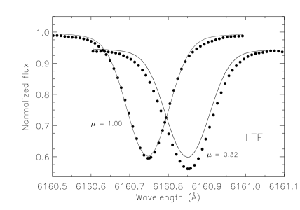
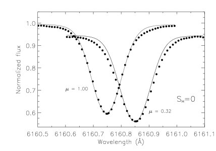
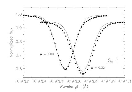
Figure 7: Center (at rest with the continuum normalized to 1) and limb (shifted to the red with the continuum normalized to 1 and subtracted 0.05) spectra for Na I $\lambda 6160.8$. Observations (filled circles) and calculations are compared for three different models: LTE, NLTE/$S_{\rm H}=0$, and NLTE/$S_{\rm H}=1$. The bottom-right panel shows the variation of the quality of the fit as a function of the position of the disk as in Fig. 6.

3.2 Na I $\lambda 6160.8$

Departures from LTE in Na I lines have also been extensively studied (e.g. Athay & Canfield 1969; Baumüller, Butler, & Gehren 1998). The level populations are again highly independent of the UV radiation field. We have used the new model atoms and calculations we previously referred to for the oxygen case. A micro-turbulence of 0.9 km s^-1 was adopted, as in Section 3.1, but a lower value of the macro-turbulence than for the oxygen triplet was necessary to fit the profiles at the center of the disk, 1.3 km s^-1, and therefore the total FWHM for the Gaussian broadening was 0.074 Å (note the difference in resolving power, as summarized in Table 1). The effective principal quantum number ($n^{*}$) of the ²S upper state is larger than 3 and therefore exceeds the range of the tables published by Anstee and O’Mara (1995). Barklem et al. (2000) derived damping cross-sections for other Na I transitions with similar energies sharing the same lower state ²P${}^{\rm o}_{3/2}$. For those transitions the FWHM of the Lorentzian (collisional) component of the line absorption profile (per unit perturber number density at 10,000 K) $\log\gamma$ was found to be in the range $-6.86$ to $-7.23$. Comparison with the observed profiles at the disk center showed that, independently of the chosen abundance, the best agreement is found for a value close to $\log\gamma=-6.86$, which was therefore adopted. Accepting $n^{*}=3$ for the upper $s$ state gives $\log\gamma=-6.96$.

Fig. 7 shows the profiles at the extreme positions ($\mu=0.32$ and 1) and the comparison with the synthetic spectra for the three cases considered. Again, we adjusted the Na abundance for each case in order to maximize the agreement between calculated and observed profiles at the center of the disk. It is evident that the sensitivity of the level populations involved in this Na I transition to collisions with H is higher than for the states connected by the O I infrared triplet. This is most likely the result of the line formation and the departures from LTE taking place in this case in higher layers. The LTE response function to the temperature for the core of the O I triplet lines peaks at $\log\tau_{\rm 5000}\simeq 0$, while that for the core of the Na I $\lambda$6160.8 line does so at $\log\tau_{\rm 5000}\simeq-1$. Using the Van Regemorter (1962) and Drawin approximations, for a typical transition of a few electron volts the ratio of the collisional rate coefficients q_H/q${}_{\rm e}\propto(U+2)/U^{2}e^{-U}/E_{1}(U)$, where $U=E_{ij}/(kT)$, and $E_{1}$ is the first-order exponential integral. Thus, q_H/q_e is a fairly flat function of the temperature or the optical depth in the solar photosphere. Between $\log\tau_{\rm 5000}\simeq 0$ and $-1$, N${}_{\rm H}/$N_e increases by an order of magnitude, making the effect of collisions with hydrogen more noticeable in higher layers. Similarly to the case of the oxygen triplet, we find the best agreement with observations when departures from LTE are considered, but now the calculations that neglect collisions with hydrogen grade best, and the differences between the $S_{\rm H}=0$ and 1 cases are now more significant. Not even the NLTE $S_{\rm H}=0$ model can match the wider profile of the sodium line that is observed near the solar limb.

Figure 8: Similar to Fig. 6 for the 3D time-dependent simulation of the solar surface.

4 The O I infrared triplet lines in a time-dependent 3D model atmosphere

Modern radiation hydrodynamics simulations offer a much more realistic representation of the lower solar atmosphere than classical static model atmospheres (Stein & Nordlund 1998; Asplund et al. 2000). In the context of these, more detailed, model atmospheres, surface convection and line broadening due to small- and large-scale velocity fields are naturally included in the calculations. This makes the use of ad hoc parameters such as macro- and micro-turbulence unnecessary, and at the same time improves substantially the agreement between observed and calculated spectral line profiles.

The consideration of several more dimensions makes calculations, however, much more involved, which, with some notable exceptions, has largely limited NLTE studies to 1D modeling. However, O I is among the few ions for which the line formation in a 3D hydrodynamical model has been studied with a complex multi-level model atom. Asplund et al. (2004) have recently shown that it is necessary to consider both, departures from LTE and a 3D geometry, to find good agreement among different spectroscopic indicators of the solar photospheric oxygen abundance, finally settling a long-standing problem. Here we will use similar calculations to revisit the center-to-limb variation of these lines, which were analyzed with a 1D model in Section 3.1.

The 3D solar simulation has been described in detail in previous papers, and the NLTE line formation calculations are identical to those reported by Asplund et al. (2004). We proceed similarly to the 1D analysis. Line profiles for the O I triplet were computed for different inclinations from the vertical axis, and averaged over azimuth, time, and horizontal position. The computed NLTE profiles are the product of an average LTE profile derived from 100 snapshots covering 50 minutes of solar time, and the ratio of the NLTE and LTE line profiles derived from two snapshots. This procedure reduces the computational burden, while introducing negligible errors. The statistical equilibrium equations were solved for the two considered snapshots for two different cases: $S_{\rm H}=0$, and $S_{\rm H}=1$. Three different abundances were used in the calculations ($\log\epsilon$(O) = 8.50, 8.70, and 8.90) and later the profiles were linearly interpolated to find the best match at the disk center in each of the three cases: LTE, $S_{\rm H}=0$, and $S_{\rm H}=1$. The calculated profiles were smoothed by convolution with a Gaussian with a FWHM of 0.088 Å to account for the finite spectral resolution of the observations.

Fig. 8 is the counterpart of Fig. 6 for the 3D case. Admittedly, the computed line profiles are not perfect. In particular, significant discrepancies are noticeable around the cores of the lines. The reader should keep in mind that the lower-right panels of Figs. 6 and 8, cannot be directly compared, as the $\chi^{\prime 2}$ is normalized to unity at the minimum independently for each case: 1D and 3D. The adopted abundances were chosen to optimize the overall fit of the $\mu=1$ observations, and the agreement is considerably better in 3D than in 1D near the line wings – even though macro-turbulence is included in the 1D case and not in 3D. The refined 3D analysis strengthens what the 1D study suggested. The calculated profiles are now close enough to the observations to justify an attempt to quantify statistically the agreement. Making use of the accuracy estimate empirically derived in Section 2, we adopt $\sigma\simeq 0.01$, and evaluate $\chi^{2}=1/\sigma^{2}\sum_{\rm i=1}^{\rm n}(f_{\rm obs}-f_{\rm synth})^{2}$ for $\mu=0.32$ in the three cases. Using only the fluxes below 3% of the continuum level to avoid the interference of obvious blending features between the lines, n$=135$, and we find $\chi^{2}$= 725, 195, and 92 and therefore significance levels of 0 ($<10^{-81}$), 10^-3, and $1$, for LTE, $S_{\rm H}=0$, and $S_{\rm H}=1$, respectively.

In the 1D analyses we have avoided comparing absolute abundances, given that the effect of atmospheric inhomogeneities was neglected. Now that the triplet lines are modeled in more detail, it is tempting to examine the absolute abundances as an additional piece of evidence. The abundances found in each case to match the profiles at the center of the disk are $\log\epsilon$(O) = 8.88, 8.66 and 8.72 for LTE, $S_{\rm H}=0$, and $S_{\rm H}=1$, respectively. The $S_{\rm H}=0$ case provides the best agreement with the average value derived by Asplund et al. (2004): $8.66\pm 0.05$ dex from forbidden and permitted lines of O I and from infrared OH lines. Thus, absolute abundance and $\chi^{2}$ statistics lead to apparently opposite conclusions in the case of the oxygen triplet. We should note that the average value derived by Asplund et al. (2004) includes permitted lines analyzed in a similar manner as in this paper with NLTE line formation and $S_{\rm H}=0$. A higher oxygen abundance from allowed lines is expected for $S_{\rm H}=1$, and in that case, forbidden and permitted lines would suggest a higher abundance (8.67–8.70) than infrared OH lines (8.61–8.65) dex.

We should stress that the necessary atomic data for the NLTE calculations were independently compiled for the 1D and 3D cases, yet the qualitative agreement is excellent. Quantitatively, the abundance corrections necessary to make the LTE and NLTE equivalent widths agree are also remarkably similar in 1D and 3D. This was also found by Asplund et al. (2004) comparing the 3D calculations with 1D abundances based on MARCS model atmospheres. The impact of departures from LTE and that of surface inhomogeneities on the abundances cannot be generally decoupled, but the situation for the OI triplet, where this is actually a good approximation, makes the conclusions from our 1D analysis to be similar as those from a 3D study.

5 Summary and conclusions

The type of observations presented here, as exemplified in Sections 3 and 4, provide a stiff test of theoretical calculations of atmospheric structure and line formation in a solar-type photosphere. The potential of center-to-limb observations to guide modeling was recognized early, but consistent $\mu\neq 1$ observations covering extensive spectral regions are still missing. We have explored how these observations can constrain the effect of collisions with hydrogen atoms on the rate equations for two particular cases.

Our results for Na I $\lambda$6160.8 fall in line with the conclusion drawn from theoretical calculations by Barklem, Belyaev, & Asplund (2003) for excitation of another alkali, lithium, by inelastic collisions with H atoms (see also the discussion by Lambert 1993). Limited by the accuracy of the observations, and approximations involved in computing line profiles, we have only tested here the extreme cases of $S_{\rm H}=0$ (no collisions with H), or $S_{\rm H}=1$ (Drawin-like formula). Comparison with detailed NLTE calculations based on multidimensional time-dependent model atmospheres and improved solar observations free from scattered light may be able to answer whether or not the use of a simplified formula scaled by a constant factor ($<<1$ for Na I or Li I) is a useful approach. Our results and a quick inspection of the literature lead to the naive conclusion that such a factor would need to vary for different species. For example, the role of hydrogen collisions compared to those with electrons increases for atmospheres more metal-poor (or cooler) than solar, and Korn, Shi, & Gehren (2003) have recently found that $S_{\rm H}=3$ is needed to satisfy the iron ionization balance in several metal-poor stars.

In the case of the oxygen infrared triplet, the solar observations are best reproduced considering inelastic hydrogen collisions in the rate equations. However, the oxygen abundance obtained when hydrogen collisions are neglected (8.66 dex) is in better agreement with the abundance inferred from OH infrared lines (8.61–8.65 dex; Asplund et al. 2004) than the abundance derived from the NLTE $S_{\rm H}=1$ analysis (8.72 dex). The higher $S_{\rm H}=1$ abundance is nevertheless still consistent with the values from forbidden lines (8.67–8.69 dex). The weighted average of the abundances from permitted lines derived by Asplund et al. (2004) changes from $8.64\pm 0.02$ dex to $8.70\pm 0.04$ dex when inelastic collisions with hydrogen are considered with the Drawin-like formula. Therefore, this apparent inconsistency could signal that the abundance derived from infrared OH lines is more uncertain than the values obtained from a detailed analysis of forbidden and permitted O I lines.

We should bear in mind that the effect of collisions with hydrogen on the statistical equilibrium is not the only important uncertainty for NLTE calculations in late-type stellar atmospheres. Electron collisions, for example, are only approximately included in our models, mainly due to the lack of reliable data for particular states. Our results should be confirmed by taking into account refined data as they become available (see, e.g., Zatsarinny & Tayal 2003). In addition, the electron density in high atmospheric layers is highly uncertain even in the 3D hydrodynamical simulations, due to the assumption of LTE. Our NLTE calculations are always ‘restricted’, in the sense that the temperature and electron density are adopted from the LTE structure calculations.

The examples discussed in this paper show how the different ingredients involved in modeling spectral line formation can begin to be unraveled when high-quality observations of spatially resolved solar line profiles are compared with detailed calculations. High quality solar observations with low spatial resolution are still missing at most wavelengths and can play a crucial role guiding theory in the quest for accuracy in the interpretation of stellar spectra.