Seismology of the Accreting White Dwarf in GW Lib

Abstract

We present a first analysis of the g-mode oscillation spectrum for the white dwarf (WD) primary of GW Lib, a faint cataclysmic variable (CV). Stable periodicities have been observed from this WD for a number of years, but their interpretation as stellar pulsations has been hampered by a lack of theoretical models appropriate to an accreting WD. Using the results of Townsley and Bildsten, we construct accreting models for the observed effective temperature and approximate mass of the WD in GW Lib. We compute g-mode frequencies for a range of accreted layer masses, $M_{\rm acc}$, and long term accretion rates, $\langle\dot{M}\rangle$. If we assume that the observed oscillations are from $\ell=1$ g-modes, then the observed periods are matched when $M\approx 1.02M_{\odot}$, $M_{\rm acc}\approx 0.31\times 10^{-4}M_{\odot}$ and $\langle\dot{M}\rangle\approx 7.3\times 10^{-11}M_{\odot}$ yr^-1. Much more sensitive observations are needed to discover more modes, after which we will be able to more accurately measure these parameters and constrain or measure the WD’s rotation rate.

1. Introduction

Dwarf Novae (DN) are the subset of CVs with low time-averaged accretion rates $\langle\dot{M}\rangle\lesssim 10^{-9}M_{\odot}\ {\rm yr}^{-1}$ and thermally unstable accretion disks that lead to sudden accretion events which interrupt the otherwise quiescent state. In quiescence, the UV (and sometimes optical) emission from the binary is dominated by light from the WD surface, allowing for a measurement of the WD’s $T_{\rm eff}$. These $T_{\rm eff}$’s are much hotter than expected for a WD of the age of the binary (a few Gyr) and must be related to accretion (Sion, 1999). Calculations of the heating of the deep interior of the WD by the prolonged accretion (Townsley & Bildsten, 2004) explains the observed values of $T_{\rm eff}$ and yields a unique relationship between $\langle\dot{M}\rangle$, the WD mass, $M$, and the orbital period $P_{\rm orb}$ (Townsley & Bildsten, 2003).

GW Lib is one of the shortest orbital period CVs known, $P_{\rm orb}=77$ min (Thorstensen et al., 2002), and therefore has a very low $\langle\dot{M}\rangle\sim 5\times 10^{-11}M_{\odot}$ yr^-1 (Townsley & Bildsten, 2003). Only one disk outburst has been observed from GW Lib (González, 1983). Much later photometric observations during quiescence led to the discovery of periodic variability (van Zyl et al., 2000) similar to that of isolated WDs which pulsate due to non-radial g-modes (see Bradley 1998 for a review of the DAV WDs). The highest signal to noise photometric observations comprise two weeks of single-site data taken in 1998 with some supplement from other longitudes (van Zyl et al., 2004). There are three clear periodicities, listed in Table 1, with some evidence for mild period variability.

Table 1Observed Periods

System	Principal Period, $P$
	(seconds)
GW Lib	$236$, $377$, $646$
SDSS 1610	345, 607
SDSS 0131	$\simeq$ 330, $\simeq$ 600
SDSS 2205	$\simeq$ 330, $\simeq$ 600

Three additional CV WD pulsators have been found (Warner & Woudt, 2003; Woudt & Warner, 2004) by taking photometric time series of DN identified in the Sloan Digital Sky Survey (SDSS; Szkody et al. 2003) which show WD spectral features in the optical. These objects and their dominant periods are also listed in Table 1. At this discovery fraction we expect $\simeq$15 CV WD pulsators total by the end of the SDSS. Seismology of the CV WD pulsators provides the prospect of well-determined masses for these systems and the parameters we derive for GW Lib are the first step in this process.

Mass determinations are especially interesting due to possible implications for progenitor systems of Type Ia supernovae. Thought to be accreting WDs near the Chandrasekhar mass (Hillebrandt & Niemeyer, 2000), these progenitors are closely related to the CV population, but the precise nature of this relationship is unknown. Important clues in this mystery lie in how the masses of CV primary WDs change over the accreting lifetime of the binary, but progress is hampered by the difficulty of measuring CV primary masses (Patterson, 1998). This mass evolution, as well as probing the $M_{\rm acc}$ directly with seismology, is also important for determining how much, if any, of the original WD material has been ejected into the ISM in classical nova outbursts, contributing to the ISM metallicity (Gehrz et al., 1998).

We begin in §2 by discussing the observed properties of the WD in GW Lib and constructing accreting WD models that are consistent with the observations. Section 3 discusses the g-mode properties for the accreting model of GW Lib, and in Section 4 we show what can be learned about the accreting WD from the observed mode periods. We conclude in Section 5 with a discussion of future work.

2. Observed Properties of the White Dwarf in GW Lib

Though the periods make it clear that the oscillations in GW Lib are non-radial g-modes, without secure identification of the radial and angular quantum numbers ($n$ and $\ell$), it is difficult to carry out the seismology. Hence, we start by using the binary’s observed properties to constrain a few of the WD’s properties, thus reducing the range of possibilities we need to consider in our modeling efforts.

2.1. Limits from Distance and $T_{\rm eff}$

We use three observations: (1) the parallax (2) a $T_{\rm eff}$-$\log g$ relationship determined from the UV spectrum, and (3) the $P_{\rm orb}$. The parallax of GW Lib has been measured from the ground (Thorstensen, 2003) and gives a distance of $104^{+30}_{-20}$ pc. Current UV spectroscopic observations can only constrain $T_{\rm eff}$ and $\log g$ to a well-determined linear relationship (see Howell et al. 2002 for a discussion). In the case of GW Lib, $T_{\rm eff}/{\rm K}=14700+2000\log_{10}g_{8}$ where $g_{8}$ is the surface gravity measured in $10^{8}$ cm s^-2 (Szkody et al., 2002). By using this, the UV flux measured from the same observation, the distance, and a WD mass-radius relation we find $M=1.03$ to $1.36M_{\odot}$ from the range of allowed distances. This constraint excludes the diagonally shaded regions in Figure 1.

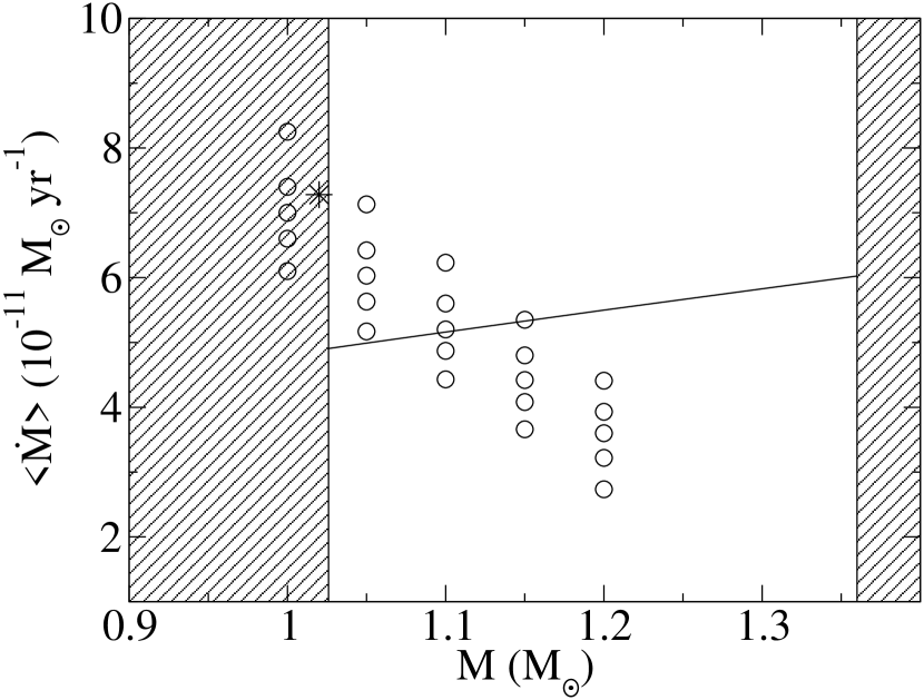
Figure 1.— Parameter space constraints from non-seismological observations. Distance, UV flux and UV spectral measurements constrain $M$ (diagonal shading) and gravitational wave radiation provides a (mass dependent) lower limit on $\langle\dot{M}\rangle$ (solid line). Actual models considered here are indicated by the circles. The $*$ indicates our best fit to the observed pulsations.

Another parameter needed is the time-averaged accretion rate, $\langle\dot{M}\rangle$. For each $M$, $P_{\rm orb}$ sets the orbital separation, and with a mass-radius relation for the Roche Lobe filling companion (we use Kolb & Baraffe’s 1999 for a low mass main sequence star) this allows a derivation of a mimimum $\langle\dot{M}\rangle$ due only to gravitational radiation from the orbit. This limit is shown by the solid line in Figure 1, and can be high if the system has passed through the period minimum, so that the companion is a sub-stellar object which is out of thermal equilibrium and has a lower mean density.

Optical spectroscopy (Szkody, Desai, & Hoard 2000; Thorstensen et al. 2002) has given lower $T_{\rm eff}$ (11000 K and 13220 K respectively), however both of these studies used gravities much lower than the allowed range derived above ($\log g=8$ and 7.4 as opposed to 8.6 for $M=1.0M_{\odot}$), and were unable to effectively account for contamination by the quiescent accretion disk, both of which would lead to low fitted $T_{\rm eff}$. The UV spectrum is the most reliable indicator of $T_{\rm eff}$.

2.2. The Accreting White Dwarf Structure

The WD interior structure is from Townsley & Bildsten (2004, hereafter TB). We chose a simple compositional structure consisting of a solar composition accreted layer of mass $M_{\rm acc}$ on the WD core, an equal mixture of ¹²C and ¹⁶O. For calculation of the buoyancy properties, a smooth transition region of $0.2$ times the local pressure scale height was put in between these layers (see TB for a discussion of the diffusion timescales). With this compositional structure, a WD model is parameterized by $M$, $T_{\rm core}$, $\langle\dot{M}\rangle$ and $M_{\rm acc}$, and compression of material by accretion powers a surface luminosity $L$. TB related $T_{\rm core}$ to $\langle\dot{M}\rangle$ by finding the equilibrium state where between classical novae outbursts (as $M_{\rm acc}$ is growing) the WD core would suffer no net heating or cooling. For a fixed $T_{\rm eff}$ at the observed value, TB also relate $\langle\dot{M}\rangle$ and $M_{\rm acc}$, with a higher $M_{\rm acc}$ implying a lower $\langle\dot{M}\rangle$ for the same $T_{\rm eff}$. Using these two constraints we are left with $M$ and $M_{\rm acc}$ as free parameters, where we only consider $M_{\rm acc}\leq M_{\rm ign}\sim 10^{-4}M_{\odot}$, the classical nova ignition mass.

This smaller grid of models are shown by the circles in Figure 1, and have $M/M_{\odot}=1.0,1.05,1.1,1.15,$ and 1.20, each with $M_{\rm acc}=0.1$, 0.3, 0.5, 0.7, and 0.9$M_{\rm ign}$. The ignition masses for these models were $M_{\rm ign}=1.40$, 1.32, 1.22, 1.14, and $1.08\times 10^{-4}M_{\odot}$. The model at $M=1.05M_{\odot}$ and $M_{\rm acc}=0.3M_{\rm ign}=0.40\times 10^{-4}M_{\odot}$ has $T_{\rm eff}=16070$ K (that implied for this $M$ by the UV spectrum), $\langle\dot{M}\rangle=6.4\times 10^{-11}M_{\odot}$ yr^-1, and $T_{\rm core}=5.9\times 10^{6}$ K. The downward trend in $\langle\dot{M}\rangle$ with increasing $M$ is due to $L$ decreasing with the WD radius with $T_{\rm eff}$ constrained to the measured relation.

3. G-modes in GW Lib’s White Dwarf

In a nonrotating star, all variables can be decomposed into spherical harmonics $Y_{lm}(\theta,\phi)$. We ignore the perturbed gravitational potential (the Cowling approximation) and work in the adiabatic approximation. The linearized momentum and energy equations are then written in terms of the radial displacement $\xi_{r}(r)$ and the Eulerian pressure perturbation $\delta p(r)\equiv\rho\psi(r)$ as (See e.g. eq.14.2 and 14.3 in Unno et al. 1989)

$$\frac{d\psi}{dr} = \frac{N^{2}}{g}\psi-(N^{2}-\omega^{2})\xi_{r}\ ,$$

$$\frac{d\xi_{r}}{dr} = -\left(\frac{1}{c^{2}}-\frac{l(l+1)}{r^{2}\omega^{2}}\right)\psi-\left(\frac{2}{r}-\frac{g}{c^{2}}\right)\xi_{r}\ .$$ (1)

Here $\omega=2\pi/P$ is the mode frequency, $P$ is the period, $c=(\Gamma_{1}p/\rho)^{1/2}$ is the adiabatic sound speed, $g=GM(r)/r^{2}$ is the downward gravitational acceleration, and $N^{2}=-g\left(d\ln\rho/dr-\Gamma_{1}^{-1}d\ln p/dr\right)$ is the square of the Brunt-Väisälä frequency. For boundary conditions, we impose zero Lagrangian pressure perturbation, $\Delta p/\rho=\psi-g\xi_{r}=0$, at the top of the model and $\xi_{r}=0$ at the interface between the solid core and surrounding liquid. This interface occurs at the freezing point for a Coulomb solid (Bildsten & Cutler 1995; Montgomery & Winget 1999) and g-modes cannot penetrate into the solid core as their frequency is too low to excite significant shearing motion of the Coulomb solid. A solid core is present in the GW Lib model due to the high mass.

Figure 2.— Comparison of propagation diagram (top panel) and WKB integrand (bottom panel) for an accreting model (solid lines) and non-accreting model (dashed line) with the same composition and $T_{\rm eff}$. The vertical solid (dashed) line on the right indicates the liquid-solid boundary. The solid horizontal lines are the observed frequencies and the dotted horizontal line is the breakup frequency. The accreting model has $M=1.05M_{\odot}$, $M_{\rm acc}=0.3M_{\rm ign}=0.40\times 10^{-4}M_{\odot}$, $T_{\rm eff}=16070$ K (that implied for this $M$ by the UV spectrum), $\langle\dot{M}\rangle=6.4\times 10^{-11}M_{\odot}$ yr^-1, and $T_{\rm core}=5.9\times 10^{6}$ K. The non-accretor has $T_{\rm core}=9.3\times 10^{6}$ K.

The propagation cavity for the observed short wavelength g-modes (Unno et al. 1989) in GW Lib is bounded from above by $\omega^{2}=L_{l}^{2}=l(l+1)c^{2}/r^{2}$, the Lamb frequency, and by the solid core below. The propagation diagram for the model with $M=1.05M_{\odot}$ and $M_{\rm acc}=0.3M_{\rm ign}=0.40\times 10^{-4}M_{\odot}$ is shown in the upper panel of Figure 2. The large peak in $N$ at $\log_{10}p\simeq 19$ is due to the change in mean molecular weight in the transition layer from the solar composition accreted envelope to the C/O core. In the roughly constant flux envelope, $N^{2}\simeq g/z$ where $z$ is the depth from the surface. In the degenerate core, $N^{2}\simeq(g/H_{p})(k_{b}T/E_{F})$, where $E_{F}$ is the electron Fermi energy and $H_{p}=p/\rho g$ is the pressure scale height. In the propagation zone of the wave, the WKB dispersion relation for low frequency g-modes gives a radial wavenumber $k_{r}=(N/\omega)[l(l+1)]^{1/2}/r$. The quantized WKB phase $\varphi$ accrued by the wave in a given region is $\varphi=\int drk_{r}=[l(l+1)]^{1/2}\omega^{-1}\int Ndr/r$ so that $\omega\propto\int NH_{p}\,d\ln p$. The integrand is shown in the bottom panel of Figure 2, representing the number of nodes per decade in pressure. Shown are two WD models: an accreting model with $M=1.05M_{\odot}$ and $M_{\rm acc}=0.3M_{\rm ign}=0.40\times 10^{-4}M_{\odot}$ used in our mode analysis (solid line), and a non-accreting model with the same $T_{\rm eff}$ (dashed line) and composition.

Not shown in Figure 2 is the difference due to the envelope mean molecular weight, $\mu$, from the case of a pure H or He envelope to one of solar compositon. Such a change is reflected in the periods as $P_{n}\propto\mu^{0.5}$, since the envelope is well-approximated by an $n=4$ polytrope. The non-accreting model also has a higher $T_{\rm core}$ than the accreting model by about 50%, leading to two important effects: (1) the WKB integrand has a higher value in the core for the non-accreting model ($\omega\propto T_{\rm core}^{1/2}$), and (2) the solid core is smaller, pushing the inner boundary condition deeper into the star. Both effects directly influence the observed periods, and period spacings, hence it is essential to use a WD model including the effects of compressional heating and nuclear burning, rather than a passively cooling WD model.

4. Inferring the WD Properties from the Periods

The existing optical time-series photometry of GW Lib (van Zyl et al., 2004) consists of 7 time series taken in 1997, 1998, and 2001. Here we focus on the best of these, the two weeks of data from May 1998. Table 1 represents our estimate of the three periods. From the $O-C$ phase plots shown by van Zyl et al. (2004), the periodicity near 646 s varies with $\dot{\nu}=\dot{\omega}/2\pi\simeq-10^{-11}$ Hz s^-1, and the phase is tracked by the observations. For that near 377 s, the phase is lost, and therefore it is inconclusive whether there are multiple closely spaced periods or just unresolved variability. The highest frequency is quite stable, and though close to a sum is unlikely to be a combination frequency. Splittings $\simeq 1$ $\mu$Hz are ubiquitous in the Fourier transforms, but their origin is unclear. The Doppler shift due to the orbit should have a magnitude of $0.5$ to 1.3 $\mu$Hz for the 646 and 236 s periods respectively. The frequency resolution set by the inverse length of the time series is also $\sim\mu$Hz.

As mentioned by van Zyl et al. (2004), the mode frequencies might drift due to the cooling of the material accreted in the last DN outburst. The magnitude and sign of this drift can be approximated using the cooling time of the freshly accreted material and its fractional contribution to the WKB integral discussed above. For a recurrence time of 20 years (the time since the last outburst) with $\langle\dot{M}\rangle\simeq 5\times 10^{-11}M_{\odot}$ yr^-1, $\Delta M\simeq 10^{-9}M_{\odot}$ was deposited in the last outburst. For $M=1.0M_{\odot}$ the base of this layer has $p_{b}\simeq 2\times 10^{14}$ dyne cm^-2, and a thermal time of $\tau_{\rm th}=c_{p}T_{b}\Delta M/L\sim 1$ yr $(p_{b}/10^{14}{\rm dyne\ cm^{-2}})^{1.2}$, implying that this layer relaxes to close to the static solution in a few years after the outburst, though a small amount of cooling continues. As can be seen from the lower panel in Figure 2, the mode frequencies are largely determined deeper in the WD; however, this outer layer does have a contribution $\int Ndz\propto p_{b}^{1/10}\propto T_{b}^{1/2}$, for an $n=4$ polytrope. This accounts for about 20% of the whole integral, and leads to $\dot{\nu}\simeq 0.2\nu\dot{T}/2T=-\nu/10\tau_{\rm th}\sim-10^{-12}{\rm Hz\ s^{-1}}$ for $\nu=1/646$ s, close enough to the observed drift to warrant further calculations of this effect, which we do not undertake here. Shorter period (lower $n$) modes reside deeper in the star, making them less vulnerable to transient heating and cooling effects.

Figure 3.— Contours in the root mean squared difference between the mode periods observed and the closest modes in the model, $\Delta P_{\rm rms}$. The best solution lies in the lower left hand corner where $M=1.02M_{\odot}$, $M_{\rm acc}=0.23M_{\rm ign}=0.31\times 10^{-4}M_{\odot}$. The dot-dashed line demonstrates approximately how $M_{\rm acc}/M_{\rm ign}$ scales with $M$ for a fixed period and $n$.

We have calculated the g-mode spectrum of model WDs with parameters on the grid indicated in Figure 1 for $\ell=1$. By interpolating within this grid we compute the model periods $P_{n}(M,M_{\rm acc})$. The root mean square period difference between the observed three modes and the models is defined as $\Delta P_{\rm rms}^{2}=\sum_{i=1}^{3}{\rm min}_{\{n\}}[(P_{n}-P_{i})^{2}]/3$, where the observed periods have been indexed with $i=1,2,3$. The contours of $\Delta P_{\rm rms}$ are shown in Figure 3, implying a best fit solution with $\Delta P_{\rm rms}=1.8$s for $M=1.02M_{\odot}$ and $M_{\rm acc}=0.23M_{\rm ign}=0.31\times 10^{-4}M_{\odot}$. The mode identifications for this best fit model are $n=3$, 8, and 17 for the three observed periods. These do not appear to correspond to any particular mode trapping pattern reflected in the mode kinetic energy. For this model, we can predict additional mode periods yet to be observed; up to $n=17$ these are 141, 191, 234, 268, 289, 310, 351, 377, 400, 432, 463, 492, 519, 553, 586, 617, 647, 678 s.

The contours for $\Delta P_{\rm rms}$ do not close around a single solution, implying additional data is needed to get better constraints. There are two other areas in the $M$-$M_{\rm acc}$ plane which also provide fairly good matches ($P_{\rm rms}<3$ s) to the observed periods. These are centered near $(M/M_{\odot},\ M_{\rm acc}/M_{\rm ign})$ of (1.06, 0.53) and (1.15, 0.6), and extend in the $M_{\rm acc}$ direction. Each of the three minima represent a different set of mode IDs, the shallower ones having $n=4$, 9, 19 and 5, 11, 22 for the 236, 377, and 646 s modes. The $M$, $M_{\rm acc}$ degeneracy can be simply explained. For a mode trapped in the envelope, $P_{n}\propto n/\int_{\rm env}Ndz\propto nM_{\rm acc}^{-0.1}M^{-2.3}$ for a polytrope of index $4$ and an assumed scaling $R\propto M^{-1.8}$, suitable for $M=1.0$ to $1.2M_{\odot}$. Thus fixing $n$ and $P_{n}$ defines the relation $M_{\rm acc}/M_{\rm ign}\propto M^{-21.5}$, where $M_{\rm ign}\propto M^{-1.5}$, leading to the degeneracy shown by the dot-dashed line in Figure 3.

5. Conclusions and Uncertainties

We have found non-rotating accreting WD models which fit the periodic variability observed in GW Lib, implying $M=1.02M_{\odot}$, $M_{\rm acc}=0.31\times 10^{-4}M_{\odot}$ and $\langle\dot{M}\rangle=7.3\times 10^{-11}M_{\odot}$ yr^-1. This model is quite simple, but since it is capable of accounting for the observed periods, a more complex model is not called for at this time. A number of important issues were not dealt with, such as the presence of a residual He layer due to inefficient nova mass ejection, or our treatment of the accreted layer-C/O boundary. More detailed non-adiabatic calculations will be undertaken to address mode excitation. The most essential omission in our calculations is the WD rotation, since it is expected to be spun up by accretion. If the WD is rapidly rotating, the model parameters derived here are likely to be inaccurate. Better observations are necessary for this next essential parameter to be constrained. These observations should accomplish two goals (1) to clearly characterize the substructure or variability of the 377 s and 646 s periods, (2) probe for lower amplitude signals. A larger number of identified modes are essential for conclusive seismology.

Rotation may significantly modify the mode frequencies. Since the maximum rotation rate for our GW Lib models is $\sim 1{\rm\ rad\ s^{-1}}$ and the observed mode frequencies are $\omega\sim 10^{-2}{\rm\ rad\ s^{-1}}$, spin frequencies above 1% breakup will cause large frequency shifts for observed modes. In fact Szkody et al. (2002) estimate $v\sin i<300\ {\rm km\ s^{-1}}$, allowing spin rates up to 6% of breakup even for high $i$. Rotation rates this large lead to a qualitative change in mode properties. When the spin frequency $\Omega_{\rm spin}\lesssim 0.5\omega$, rotation can be treated as a small perturbation. Also, observationally this rotational frequency splitting allows a determination of the $l$ quantum number. If, however, $\Omega_{\rm spin}\gtrsim 0.5\omega$, the Coriolis force has a “nonperturbative” effect on the mode frequencies, modifying the relation between the frequency and quantum numbers (Bildsten, Ushomirsky, & Cutler, 1996). Hence accreting WDs may provide a unique proving ground for techniques of seismology for rapidly rotating stars.

This work was supported by the National Science Foundation under grants PHY99-07949, AST02-05956, and 0201636, and by NASA through grant AR-09517.01-A from STScI, which is operated by AURA, Inc., under NASA contract NAS5-26555. Phil Arras is a NSF AAPF fellow.

References

- Bildsten & Cutler (1995) Bildsten, L. & Cutler, C. 1995, ApJ, 449, 800
- Bildsten et al. (1996) Bildsten, L., Ushomirsky, G., & Cutler, C. 1996, ApJ, 460, 827
- Bradley (1998) Bradley, P. A. 1998, Baltic Astronomy, 7, 111
- Gehrz et al. (1998) Gehrz, R. D., Truran, J. W., Williams, R. E., & Starrfield, S. 1998, PASP, 110, 3
- González (1983) González, L. E. 1983, IAU Circ, 3854
- Hillebrandt & Niemeyer (2000) Hillebrandt, W. & Niemeyer, J. C. 2000, ARA&A, 38, 191
- Howell et al. (2002) Howell, S. B., Gänsicke, B. T., Szkody, P., & Sion, E. M. 2002, ApJ, 575, 419
- Kolb & Baraffe (1999) Kolb, U. & Baraffe, I. 1999, MNRAS, 309, 1034
- Montgomery & Winget (1999) Montgomery, M. H. & Winget, D. E. 1999, ApJ, 526, 976
- Patterson (1998) Patterson, J. 1998, PASP, 110, 1132
- Sion (1999) Sion, E. M. 1999, PASP, 111, 532
- Szkody et al. (2000) Szkody, P., Desai, V., & Hoard, D. W. 2000, AJ, 119, 365
- Szkody et al. (2002) Szkody, P., Gänsicke, B. T., Howell, S. B., & Sion, E. M. 2002, ApJ, 575, L79
- Szkody et al. (2003) Szkody, P. et al. 2003, AJ, 126, 1499
- Thorstensen (2003) Thorstensen, J. R. 2003, AJ, 126, 3017
- Thorstensen et al. (2002) Thorstensen, J. R., Patterson, J., Kemp, J., & Vennes, S. 2002, PASP, 114, 1108
- Townsley & Bildsten (2003) Townsley, D. M. & Bildsten, L. 2003, ApJ, 596, L227
- Townsley & Bildsten (2004) —. 2004, ApJ, 600, 390, TB
- Unno et al. (1989) Unno, W., Osaki, Y., Ando, H., Saio, H., & Shibahashi, H. 1989, Nonradial oscillations of stars (Nonradial oscillations of stars, Tokyo: University of Tokyo Press, 1989, 2nd ed.)
- van Zyl et al. (2000) van Zyl, L., Warner, B., O’Donoghue, D., Sullivan, D., Pritchard, J., & Kemp, J. 2000, Baltic Astronomy, 9, 231
- van Zyl et al. (2004) van Zyl, L. et al. 2004, To appear in MNRAS, (astro-ph/0401459)
- Warner & Woudt (2003) Warner, B. & Woudt, P. A. 2003, in ASP Conf. Ser. 2nn: Variable Stars in the Local Group, ed. D. W. Kurtz & K. Pollard, (astro-ph/0300072)
- Woudt & Warner (2004) Woudt, P. A. & Warner, B. 2004, MNRAS, 348, 599