Altair: The Brightest Delta Scuti Star

Abstract

We present an analysis of observations of the bright star Altair ($\alpha$ Aql) obtained using the star camera on the Wide-Field Infrared Explorer (WIRE) satellite. Although Altair lies within the $\delta$ Scuti instability strip, previous observations have not revealed the presence of oscillations. However, the WIRE observations show Altair to be a low-amplitude ($\Delta m<1$ ppt) $\delta$ Scuti star with at least 7 modes present.

1 Introduction

Delta Scuti stars are a variety of pulsating variable star located within the classical instability strip of the HR diagram (Rodriguez & Breger 2001). They inhabit the region between $3.8<\log\rm T_{eff}<3.95$ and $0.6<\log\rm(L/L_{\sun})<2.0$, and display periods ranging from 0.02 to 0.3 days. Some belong to the high-amplitude $\delta$ Scuti (HADS) class, which display $V$ amplitudes in excess of 0.3 mag, and generally oscillate in radial modes, while the lower-amplitude members of the class have more complex frequency structure, typically showing numerous nonradial modes.

Altair ($\alpha$ Aql) is an A7 IV-V main sequence star (Johnson & Morgan 1953) and is the 12th brightest star in the sky (V = 0.755, Cousins 1984). While it lies inside the instability strip, we are unaware of any reports of photometric variability. Erspamer & North (2003) report $\rm T_{eff}=7550K$ and $\log g=4.13$, and Zakhozhaj (1979, see also Zakhozhaj & Shaparenko 1996) derives a mass of $1.75M_{\sun}$ and a radius of $1.58R_{\sun}$ based on photometry. The Hipparcos parallax for Altair is $194.44\pm 0.94\rm~{}mas$, giving a distance of $5.143\pm 0.025\rm~{}pc$. Combined with the observed V magnitude and the bolometric correction from Flower (1996) gives $\rm M_{bol}=2.18$. Altair is a rapid rotator, with spectroscopically derived $v\sin i$ values in the literature ranging from $190\rm~{}km~{}s^{-1}$ to $250\rm~{}km~{}s^{-1}$ (Royer et al. 2002).

Altair is nearby enough to make direct measurement of its diameter possible. Richichi et al. (2002) reported a diameter of $3.12\rm~{}mas$, corresponding to a radius of $1.72\rm R_{\sun}$. Recent interferometric observations (Van Belle et al. 2001) have established that Altair is oblate, with equatorial diameter of $3.46\rm~{}mas$ (corresponding to a radius of $1.9\rm R_{\sun}$) and polar diameter of $3.037\rm~{}mas$, for an axial ratio $a/b=1.14\pm 0.029$. Van Belle et al. also derive a value for $v\sin i$ of $210\pm 13\rm~{}km~{}s^{-1}$.

Altair’s absolute V magnitude is +2.22 (based on the Hipparcos distance) and its $\rm(b-y)_{0}=0.137$ (Hauck & Mermilliod 1998; Nekkel et al. 1980), which places it well inside the $\delta$ Scuti instability strip (Breger 1990). However, like many such objects, Altair has never been detected to oscillate. It is as yet unclear whether these non-oscillating stars within the instability strip are truly non-oscillating, or whether the non-detections are instead due to either periods or amplitudes which are undetectable from the ground; some indications are that slow rotation is a necessary condition for large oscillation amplitudes (Breger 1982, Solano & Fernley 1997, but for an alternate view see Rasmussen et al. 2002).

2 Observations and Data Reduction

The Wide-Field Infrared Explorer (WIRE) mission was launched by NASA into a sun-synchronous orbit on 4 March 1999. The primary mission failed several days after launch, but conversion of the spacecraft into an asteroseismology platform using the onboard star camera as the new science instrument began on 30 April 1999.

The star camera consists of a 52 mm, f/1.7 refractive optic feeding a $512^{2}$ SITe CCD and a 16-bit analog-to-digital converter. The camera has a field of view of roughly 7.8 degrees square, corresponding to an image scale of 1 arc minute per pixel; it is unfiltered, but the effective response is roughly $\rm(V+R)$. Observations of Altair were carried out with a cadence of 0.5 seconds. Details of the instrument and its performance can be found in Buzasi (2000, 2002, 2003).

Altair was observed from 18 October through 12 November 1999. Exposures of 0.1 second were taken during about 40% of the spacecraft orbital period. Some additional gaps due to mission operations constraints were also present, resulting in an overall duty cycle of approximately 27%.

We have reduced the data using two independent techniques, which we now describe. In the first approach, as described in Buzasi (2000), data reduction began by applying a simple aperture photometry algorithm, which simply involved summing the central $4\times 4$ pixel region of the $8\times 8$ pixel field of view. The background level, due primarily to scattered light from the bright Earth, was estimated based on the four corner pixels of each image, and subtracted. A total of approximately 1.27 million data points were acquired during the observing window.

Following aperture photometry, a clipping algorithm was applied to the time series, resulting in the rejection of any points deviating more than $2.5\sigma$ from the mean flux, image centroid, or background level. In practice, at this point in the data reduction process, the rms noise in the signal is extremely large ($\sigma\approx 12$ ppt) due to incomplete subtraction of scattered light, so clipping in this way only removes truly deviant points. The majority of these are due to either data from the wrong 8x8 CCD “window” being returned, or to data acquired before the spacecraft pointing had settled during a particular orbital segment. After this stage, approximately 1.21 million data points remained.

As noted in the previous paragraph, the crude scattered light removal discussed above is clearly inadequate. Much of the difficulty inherent in the reduction of WIRE photometric data is in successfully characterizing and removing the scattered light signature (Buzasi 2000). We phased the data at the satellite orbital period, binned the result in steps of phase $10^{-3}$, and fit and subtracted a spline to the result, which lowered the rms noise level by approximately an order of magnitude. For an example of this process, see Retter et al. (2003).

The resulting distribution of magnitudes is a Gaussian with some outliers. We discarded 466 points that were more than $4\sigma$ from the mean, and then binned into $50\rm~{}s$ intervals, discarding bins containing fewer than 20 points. To remove slow trends, we also fitted and subtracted a third-order polynomial. The final binned time series contained 9828 points.

In the second approach we first fit a 2D-Gaussian profile to each $8\times 8$ image in order to examine changes in the central $(x,y)$ position of the stellar profile and to find out how the FWHM changes. The $(x,y)$ position of the main target is found to be extremely stable, ie. $x=3.271\pm 0.006$ and $y=3.158\pm 0.008$, where $(x,y)=(3.5,3.5)$ is the center of of the $8\times 8$ window. The FWHM of the stellar profile is also very stable, $F=1.860\pm 0.003$ pixels.

For each image we measured the stellar flux using aperture photometry. The sky level was determined by the average flux of the four pixels in the corners of the CCD image, and the aperture was centered on the $(x,y)$ position found from the Gaussian 2D-fit. The aperture sizes were scaled with the FWHM of the fitted Gaussian to ensure that approximately the same region of the PSF profile is sampled. To ensure robustness, the sky background, the $(x,y)$ position, and the FWHM we used were the average of the preceding 20 and following 20 images, thus averaging over a full 20 seconds.

We used eight different apertures with increasing radii, and found the lowest noise when applying an aperture with radius $r=1.39F$, corresponding to $r=2.52$ pixels.

We binned the light curve into groups of $n=51$ data points, requiring that each $(x,y)$ position be within 0.1 pixels of the mean; 3 $\sigma$ outliers were removed. We also required that the time interval between subsequent data points not exceed 10 seconds. The resulting light curve has 40 088 data points. The original data points have a point to point noise of 0.73 ppt, while in the binned light curve the noise is 0.16 ppt.

We note that after subtracting the detected oscillation modes (cf. Section 3) we detected a slight correlation with the FWHM and have removed this by fitting a second degree polynomial to the residual flux vs. FWHM.

The entire Altair light curve is shown in Figure 1, while Figure 2 zooms in on a portion. In the latter figure, the fit is overlaid as a solid curve.

Figure 1: The complete observed light curve of Altair. The time is the heliocentric Julian date relative to the time $t_{0}=2\,451\,480$, and individual panels are labeled according to range of days they encompass relative to that date.

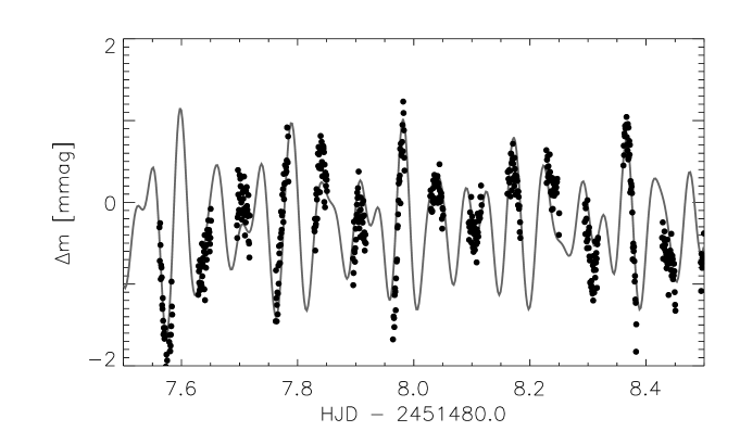
Figure 2: 18 hours of the observed light curve of Altair. The solid curve is the fit to the light curve, based on the frequencies shown in Table 1. The time is the heliocentric Julian date relative to the time $t_{0}=2\,451\,480$.

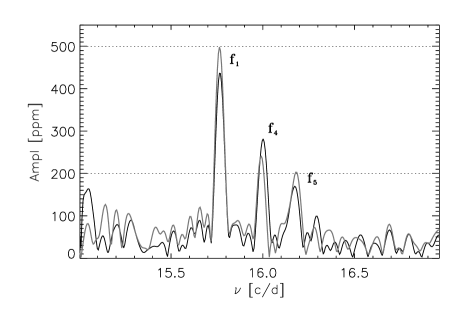
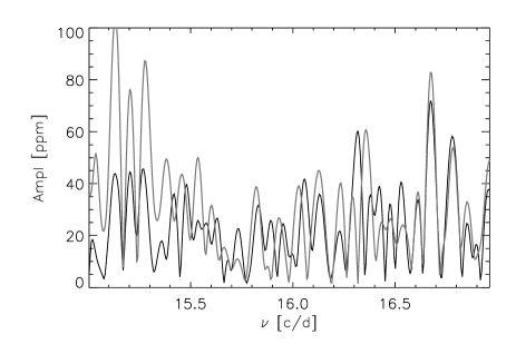
Figure 3: The left panel shows the amplitude spectra of the light curve of Altair in the range 15.3–16.6 c/day. The gray and black colors correspond to the first and second data reduction techniques (see text for details). In the right panel the three main modes have been subtracted from the light curve. While the apparent amplitude is larger for the “gray” spectrum the noise level is also significantly higher. The horizontal dotted lines are added to aid the eye.

3 Analysis

Figure 3 shows the a portion of the amplitude spectrum for the light curve extracted as described in Section 2. In the left panel the oscillation signal around 16.0 c/day can be seen. The right panel shows the amplitude spectrum when the three detected modes are removed.

Note that in both data sets a slow drift has been observed corresponding to a peak in the amplitude spectrum at a period of 27.0 days and an amplitude of just 320 ppt. Due to aliasing this will give rise to a group of peaks around $f_{\rm alias}=f_{\rm orb}-f_{0}$, where $f_{\rm orb}$ is the orbital frequency of WIRE, ie. 15.00 c/day. This is just below the frequency of the three observed peaks in the amplitude spectrum and with comparable amplitudes.

After removing the oscillation signal from the light curves we measured the noise level in the amplitude spectrum. In the high frequency range (30–60 c/day) the Buzasi (2000) approach (technique 1; gray curve) gives a noise level of 10.5 ppm, while our new approach (technique 2; black curve) gives a noise level of 9.8 ppm. In the range 15–17 c/day (around the oscillation peaks) we find 26.6 and 21.0 ppm, respectively. Thus, the noise levels are comparable at high frequencies but significantly lower for the second method at the lower frequencies. The apparently higher amplitude of the three oscillation modes (see left panel of Figure 3) derived from technique 1 is due to this higher noise level.

Figure 4 shows the amplitude spectrum of Altair from the second reduction method. We identify seven modes in this spectrum. Note that both reduction methods yield identical oscillation frequencies within the estimated uncertainties.

Figure 4: Amplitude spectrum of Altair in the range 15.5 – 26.5 c/day. The seven modes have been labeled. Note that the $f_{7}$ peak lies to the left of the label; compare to Figure 5. The horizontal dotted line is added to aid the eye.

Figure 5: The amplitude spectrum of Altair in the range 15.5 – 26.5 c/day, prewhitened to remove frequencies $f_{1}$ – $f_{5}$. The significance of the peaks we identify as $f_{6}$ and $f_{7}$ is clearly apparent.

Table 1 shows for each oscillation mode the frequency, amplitude, phase, and signal to noise ratio for the two different techniques. We used the software period98 (Sperl 1998) to determine the mode parameters. The phase corresponds to the heliocentric Julian date $t_{0}=2\,451\,480$ and the phase $\phi$ is in units of $2\pi$, thus, the light curve fit shown in Figure 2 is represented by $\delta m=\sum_{i=1}^{7}A_{i}*\sin(2\pi[f_{i}*(t-t_{0})+\phi_{i}])$. We estimate amplitude errors to be of the order of $\pm 20$ ppm; this is apparent from a comparison of the amplitude of $f_{2}$ in Figure 4 to that derived from period98 and shown in Table 1. Frequency errors are approximately $\pm 0.001\rm~{}c/d$.

Table 1: Parameters of the observed oscillation modes in Altair.

	$\nu$ [c/d]	$A$ [ppm]	$\phi$	(S/N)1	(S/N)2
$f_{1}$	15.768	413	0.383	19.7	23.3
$f_{2}$	20.785	373	0.299	28.6	28.5
$f_{3}$	25.952	244	0.141	19.2	18.7
$f_{4}$	15.990	225	0.689	8.7	12.6
$f_{5}$	16.182	139	0.461	7.5	7.8
$f_{6}$	23.279	111	0.102	8.0	8.5
$f_{7}$	28.408	132	0.553	7.4	7.4

4 Discussion

The accepted definition of a $\delta$ Scuti star (Breger 1979, Rodríguez et al. 1994) is a variable star with spectral type between A2 and F0, oscillation periods less than $0.3\rm~{}d$, and visual amplitudes typically less than $0.3\rm~{}mag$. SX Phe stars are similar to $\delta$ Scuti in most respects, but show Population II characteristics combined with anomalously large masses and young ages, while $\lambda$ Bootis stars combine $\delta$ Scuti-type oscillations with abundance anomalies in Fe, C, N, O, and S. Since Altair shows neither abundance anomalies nor Pop II characteristics (indeed, it lies towards the low-mass end of the instability strip), and has spectral type A7 IV-V and primary oscillation period 0.0634 days, we identify it as a $\delta$ Scuti star. In the following we will compare the observed oscillation modes with a number of published models with parameters close to Altair. However, we stress that these models do not take into account rotation, which will significantly change the structure of the star. In a future paper we will address the detailed modeling of Altair.

Using the basic pulsation relation

$$P\sqrt{\rho/\rho_{\sun}}=Q$$ (1)

where $P$ is the pulsation period, $\rho$ the mean stellar density, and $Q$ the pulsation constant, it is straightforward to derive a theoretical period-luminosity relation of the form (Breger & Bregman 1975)

$$\log Q=-6.454-\log f+0.5\log g+0.1M_{bol}+\log T_{e}$$ (2)

where frequency $f$ is in $\rm d^{-1}$. The pulsation constant $Q$ varies depending on both stellar structural considerations and the specific mode in question, but for the radial fundamental mode $Q=0.033\rm~{}d$ for $\delta$ Scuti stars (Breger 1979). Using our fundamental parameters for Altair from Section 1, we then predict the frequency of the fundamental mode to be $15.433\rm~{}d^{-1}$, remarkably close to our observed $f_{1}=15.768\rm~{}d^{-1}$.

Extensive linear and nonlinear analysis of $\delta$ Scuti oscillation properties has been published (see, e.g. Bono et al. 1997, Milligan & Carson 1992, Andreasen, Hejlesen, & Petersen 1983, Stellingwerf 1979, and references therein). Use of these model grids allows us to further clarify the mode identification in Altair.

Stellingwerf (1979) calculated a grid of models intended to represent both dwarf Cepheids and $\delta$ Scuti stars. His models 4.2 and 4.3 appear to best represent Altair on the basis of global physical properties. Model 4.2 has $\rm M=2.0M_{\sun}$, $\rm T_{e}=7700\rm K$, $\rm R=2.03R_{\sun}$, and $\log\rm g=4.12$, while model 4.3 is somewhat smaller ($\rm R=1.88R_{\sun}$) and hotter ($\rm T_{e}=8000\rm K$). Both models have $X=0.7$, $Z=0.02$. Table 2 shows the comparison between our observations and Stellingwerf’s models for our $f_{1}$, $f_{2}$, and $f_{3}$. Overall agreement is quite good, with our observations generally lying between the model predictions. Stellingwerf’s models also predicted that the third overtone should also be visible, at a frequency between $27.701$ and $31.056\rm~{}d^{-1}$. There is no conclusive evidence in our amplitude spectrum for such a mode, though the location of our $f_{7}$ is certainly suggestive.

Milligan & Carson (1992) calculated a grid of $\delta$ Scuti oscillation frequencies based on evolved Kippenhahn et al. (1967) interiors models. They label models both by mass and age. Their $1.6\rm M_{\sun}$ models are the best fit to Altair in terms of global observable parameters; model m16e02 has $\rm T_{e}=7765\rm K$ and $\log\rm g=4.21$, model m16e03 has $\rm T_{e}=7560\rm K$ and $\log\rm g=4.15$, and model m16e04 has $\rm T_{e}=7285\rm K$ and $\log\rm g=4.08$. The usage is such that m16e01 has mass $\rm 1.6M_{\sun}$ and $\log\tau=2.6$, where age $\tau$ is measured in units of $10^{6}$ years; m16e03 has $\log\rm~{}age=2.7$, and m16e04 has $\log\rm~{}age=2.8$. Table 2 gives the comparison between our measured frequencies and those predicted by Milligan & Carson for the three largest amplitude modes.

Table 2: Parameter Comparison to the models of Stellingwerf (1979) and Milligan & Carson (1992). Model labels are described in the text.

Parameter	Measured	4.2	4.3	m16e02	m16e03	m16e04
$f_{1}$	15.768	14.641	16.340	18.5235	16.6514	14.6556
$f_{2}$	20.785	18.692	20.833	24.4240	21.8936	19.2231
$f_{3}$	25.952	23.095	25.840	30.4406	27.2681	23.9363
$\Pi_{1}/\Pi_{0}$	0.75862	0.78328	0.78433	0.75841	0.76056	0.76240
$\Pi_{2}/\Pi_{0}$	0.60758	0.63395	0.63235	0.60852	0.61066	0.61227
$Q_{0}$	0.03230	0.03479	0.03117	0.03244	0.03253	0.03256
$Q_{1}$	0.02451	0.02725	0.02445	0.02460	0.02474	0.02482
$Q_{2}$	0.01963	0.02205	0.01971	0.01974	0.01986	0.01994

Milligan & Carson also used nonlinear models to investigate oscillation amplitudes for a number of their models, including m16e03. In each case, they searched for an initial velocity amplitude that would give a settled pulsation with constant maximum kinetic energy per period. For the case of m16e03, they found that the resulting second overtone frequency was $26.67\rm~{}d^{-1}$ – similar to that of the linear calculation – and that the required velocity amplitude was $100\rm~{}m~{}s^{-1}$, corresponding to an approximate $V$ amplitude of $0.5$ ppt. Both results are quite close to those determined from our observations. We note that spectroscopic detection of such a small velocity amplitude would be quite challenging, though certainly within the current state of the art (Butler 1998).

Figures 4 and 5 and Table 1 show the presence of four additional peaks ($f_{4}$ – $f_{7}$) in the amplitude spectrum with semi-amplitudes greater than $100$ ppm. $f_{4}$ and $f_{5}$ are located near the frequency of the radial fundamental mode, but are well-separated in frequency space. Given their frequencies, these peaks must correspond to nonradial oscillation modes, but beyond that our identification is uncertain. The identifications of $f_{6}$ and $f_{7}$ are likewise uncertain, although we tentatively identify $f_{7}$ with the third radial overtone.

More modern models of $\delta$ Scuti stars, incorporating OPAL and OP opacities, were explored by Petersen & Christensen Dalsgaard (1996, 1999). Updated versions of the stellar model sequences used in these papers were published online by Petersen (1999), and we compared our frequencies to these results. Unfortunately, the metallicity of Altair appears to be somewhat uncertain; the value given in Cayrel de Stroebel et al. (1992) is actually that of $\alpha$ Aqr rather than $\alpha$ Aql. However, Zakhozhaj & Shaparenko (1996) and Erspamer & North (2003) give $\rm[Fe/H]=-0.24$, while use of the TempLogG tool (http://ams.astro.univie.ac.at/templogg/) together with Strömgren photometry gives $\rm[Fe/H]=-0.15$, so we have chosen to compare our data to Petersen’s models with $Z=0.02$ (equivalent to $\rm[Fe/H]=-0.16$).

The effective temperature and bolometric magnitude of Altair fall slightly below Petersen’s $1.8M_{\sun}$ evolutionary track, a result which is in accord with Erspamer & North’s value of $1.75M_{\sun}$. In addition, Petersen’s Figure 4 allows us to estimate the stellar mass based on $(\log T_{eff},\log\Pi_{0})$ – the result once again is $M\approx 1.75M_{\sun}$.

Our first harmonic, however, does not fit well onto Petersen’s $(\log\Pi_{0},\Pi_{1}/\Pi_{0})$ diagram. In particular, for our value of $\log\Pi_{0}=-1.198$, all Petersen’s models with $Z=0.02$ fall in the range $\Pi_{1}/\Pi_{0}=0.771-0.773$, quite different from our measured value of 0.759. We suspect that this difference is due to the fact that Petersen’s models were calculated in the absence of rotation, while Altair is an extremely rapid rotator. We can estimate the frequency shift due to rotation by using Saio’s (1981) polytropic models (see also Perez Hernandez et al. 1995 for a similar application). We take the frequency shift to be

$$\nu_{n00}-\nu_{n0}^{(0)}=(Z_{n0}+X_{0})\frac{\nu_{rot}^{2}}{\nu_{n0}^{(0)}}$$ (3)

where $\nu_{nlm}$ is the frequency of the mode with radial order $n$, degree $l$, and azimuthal order $m$, $\nu_{nl}^{(0)}$ is the frequency of the same mode in a non-rotating star, $\nu_{rot}$ is the stellar rotational frequency (rigid body rotation is assumed), and the coefficients $X_{0}$ and $Z_{nl}$ are structural coefficients. Here $X_{0}\approx 1.333$ and the the $Z_{n0}$ are estimated by interpolation from the values in Saio (1981). The result indicates frequency shifts in the direction of lower frequencies, on the order of a few percent for the fundamental mode and nearly 10% for the first harmonic. In addition, the prescription of Saio does not take into account departures from rigid body rotation that likely occur for extremely high rotation rates (in this case, for example, $\Pi_{0}/\Omega\approx 0.15$). It is thus unsurprising that the period ratios from Petersen do not correspond well to our measured values; perhaps the larger surprise is that the period of the fundamental mode seems to fit so well! We note without comment that assuming $M=1.8M_{\sun}$ and fitting to Petersen’s evolutionary tracks in the $(\log\Pi_{0},\log\rm Age)$ domain yields an age for Altair of $630\pm 50$ Myr, which in turn is in accord with the A7 IV-V spectral type generally assigned to Altair.

5 Conclusions

We have determined that the bright A7 IV-V star Altair is an oscillating variable of the $\delta$ Scuti type, and that its three most significant oscillation frequencies correspond well to the fundamental radial mode and its first two overtones. Four additional frequencies are present at lower amplitudes, and these may represent nonradial modes. Our result suggests that oscillation may in fact be present in many putatively “non-oscillating” stars in the instability strip.

On the basis of the observed frequencies and the model fits, several specific points are clear:

1. As suggested by the theoretical P-L relation of Breger & Bregman (1975), the highest-amplitude mode is the radial fundamental mode. The amplitude of this oscillation, 0.5 ppt, is several times smaller than is typically detected in non-HADS $\delta$ Scuti stars from ground-based observations. The first and second overtones are also apparent.

2. It has been suggested that (Breger 1982) that slow rotation is a necessary (but not sufficient) condition for the development of large-amplitude oscillations in $\delta$ Scuti stars. Our result supports this contention.

3. A number of authors (see, e.g. Rasmussen et al. 2002 and references therein) have tried to understand the excitation mechanism in $\delta$ Scuti stars by searching for systematic differences between variable and non-variable stars. Our result suggests that such searches may be complicated by the fact that “non-variable” stars may in fact be variable at levels undetectable from the ground. In fact, the division between “variable” and “non-variable” stars in the instability strip may truly be an observational (detection technology-limited) one, with the objects in question occupying a broad continuum of photometric amplitudes.

4. Non-rotating models should not be expected to yield accurate representations of oscillation frequencies or ratios in rapidly rotating $\delta$ Scuti stars. There is a significant need for calculations of oscillation frequencies that incorporate the effects of rotation.

References

- (1) Andreasen, G.K., Hejlesen, P.M. & Petersen, J.O. 1983, A&A, 121, 241
- (2) Bono, G., Caputo, F., Cassisi, S., Castellani, V., Marconi, M., & Stellingwerf, R.F. 1997, ApJ, 477, 346
- (3) Breger, M. 1979, PASP, 91, 5.
- (4) Breger, M. 1982, PASP, 94, 845.
- (5) Breger, M. 1990, in “Confrontation Between Stellar Pulsation and Evolution,” (San Francisco: ASP), 263-273
- (6) Breger, M. & Bregman, J.N. 1975, ApJ, 200, 343
- (7) Butler, R. P. 1998, ApJ, 494, 342
- (8) Buzasi, D.L. 2000, in “The Third MONS Workshop: Science Preparation and Target Selection, ” eds. T.C. Teixeira & T.R. Bedding, 9
- (9) Buzasi, D. 2002, in “Radial and Nonradial Pulsations as Probes of Stellar Physics,” IAU Colloquium 185, eds. C. Aerts, T. R. Bedding, & J. Christensen-Dalsgaard (San Francisco: ASP), 616.
- (10) Buzasi 2003, in “Proceedings, Second Eddington Workshop,” in press.
- (11) Cayrel de Stroebel, G., Hauck, B. Francois, P, Thevenin, F., Friel, E., Mermilliod, M., & Borde, S. 1992, A&AS, 95, 273
- (12) Cousins, A.W.J. 1984, SAAO Circ. 8, 59
- (13) Erspamer, D. & North, P. 2003, A&A, 398, 1121
- (14) Flower, P. J. 1996, ApJ, 469, 355
- (15) Hauck, B. & Mermilliod, M. 1998, A&AS, 129, 431
- (16) Johnson, H.L. & Morgan, W.W. 1953, ApJ, 117, 313
- (17) Kippehnhahn, R., Weigert, A., & Hofmeister, E. 1967, in “Methods in Computational Physics 7,” eds. B. Alder, S. Fernbach, & M. Rotenburg (New York: Academic), 129.
- (18) Milligan, H. & Carson, T.R. 1992, ApJS, 189, 181
- (19) Neckel, T., Klare, G., & Sarcander, M. 1980, Bull. D’Inf. Cent. Donnees Stellaires, 19, 61.
- (20) Perez Hernandez, F., Claret, A., & Belmonte, J.A. 1995, A&A, 295, 113
- (21) Petersen, J.O. & Christensen Dalsgaard, J. 1996, A&A, 312, 463
- (22) Petersen, J.O. & Christensen Dalsgaard, J. 1999, A&A, 352, 547
- (23) Retter, A., Bedding, T.R., Buzasi, D.L., Kjeldsen, H., Kiss, L.L. 2003, ApJ, 591, L151
- (24) Richichi, A. & Percheron, I. 2002, A&A, 386, 492
- (25) Rasmussen, M.B., Bruntt, H., Frandsen, S., Paunzen, E., & Maitzen, H.M. 2002, A&A, 390, 109
- (26) Rodríguez, E. & Breger, M. 2001, A&A, 366, 178
- (27) Rodríguez, E. Lopez de Coca, P., Rolland, A., Garrido, R., & Costa, V. 1994, A&AS, 106, 21
- (28) Royer, F., Grenier, S., Baylac, M.-O., Gomez, A.E., & Zorec, J. 2002, A&A, 393, 897
- (29) Saio, H. 1981, ApJ, 244, 299
- (30) Solano, E. & Fernley, J. 1997, A&AS, 122, 131
- (31) Sperl, M. 1998, Comm. in Asteroseismology (University of Vienna), 111, 1.
- (32) Stellingwerf, R.F. 1979, ApJ, 227, 935
- (33) Van Belle, G.T., Ciardi, D.R., Thompson, R.R., Akeson, R.L., & Lada, E. 2001, ApJ, 559, 1155
- (34) Zakhozhaj, V.A. & Shaparenko, E.F. 1996, Kinematika Fiz. Nebesn. Tel., 12, 20-29.