An intense soft-excess and evidence for light bending in the luminous narrow-line quasar PHL 1092

Abstract

The narrow-line quasar PHL 1092 was observed by XMM-Newton at two epochs separated by nearly thirty months. Timing analyses confirm the extreme variability observed during previous X-ray missions. A measurement of the radiative efficiency is in excess of what is expected from a Schwarzschild black hole. In addition to the rapid X-ray variability, the short UV light curves ($<$ 4 hours) obtained with the Optical Monitor may also show fluctuations, albeit at much lower amplitude than the X-rays. In general, the extreme variability is impressive considering that the broad-band (0.4–10 keV rest-frame) luminosity of the source is $\sim$ 10⁴⁵ erg s^-1. During at least one of the observations, the X-ray and UV light curves show common trends, although given the short duration of the OM observations, and low significance of the UV light curves it is difficult to comment on the importance of this possible correlation. Interestingly, the high-energy photons ($>$ 2 keV) do not appear highly variable. The X-ray spectrum resembles that of many narrow-line Seyfert 1 type galaxies: an intense soft-excess modelled with a multi-colour disc blackbody, a power-law component, and an absorption line at $\sim$ 1.4 keV. The $\sim$ 1.4 keV feature is curious given that it was not detected in previous observations, and its presence could be related to the strength of the soft-excess. Of further interest is curvature in the spectrum above $\sim$ 2 keV which can be described by a strong reflection component. The strong reflection component, lack of high-energy temporal variability, and extreme radiative efficiency measurements can be understood if we consider gravitational light bending effects close to a maximally rotating black hole.

1 Introduction

The narrow-line quasar PHL 1092 ($z=0.396$) was observed by XMM-Newton as part of the Guaranteed Time Program to study Narrow-Line Seyfert 1 type objects (NLS1). The importance of PHL 1092 was realised by Bergeron & Kunth (1980) when it appeared unique among a sample of quasars due to its outstanding Fe II emission. During the $ROSAT$ era PHL 1092 was recognised as a high-luminosity analogue of the NLS1 phenomenon (Forster & Halpern 1996; Lawrence et al. 1997). Remarkable variability was observed during an 18-day ROSAT HRI monitoring campaign (Brandt et al. 1999; hereafter BBFR), including a number of high-amplitude flaring events. The most extreme variability was an increase in the rest-frame count rate by nearly a factor of four in less than 3580 s, corresponding to a radiative efficiency (Fabian 1979; see also Section 4.1) of $\eta$ $>$ 0.63. Such extreme variability had never before been observed in such a high-luminosity radio-quiet quasar.

The objectives of this study are to determine if PHL 1092 consistently exhibits such extreme behavior, and to constrain better the physical nature of its X-ray spectral energy distribution.

2 Observation and data reduction

PHL 1092 was observed with XMM-Newton (Jansen et al. 2001) on two separate occasions. The first observation occurred on 2000 July 31 during revolution 0118 and lasted for $\sim$ 32 ks. During this time the EPIC pn (Strüder et al. 2001) and MOS (MOS1 and MOS2; Turner et al. 2001) cameras, as well as the Optical Monitor (OM; Mason et al. 2001) and the Reflection Grating Spectrometers (RGS1 and RGS2; den Herder et al. 2001) collected data. From this first observation EPIC, OM, and RGS event files were created and supplied by the XMM-Newton Science Operations Centre. On analysing the EPIC data it was found that problems with the energy calibration existed. As such, the EPIC spectra could not be exploited due to calibration uncertainties within the small energy bins utilised for spectral analyses. Fortunately, broad-band light curves are not as sensitive to calibration uncertainties as spectra; hence it was possible to construct a pn light curve from these data. RGS and OM files were not affected. Since the Observation Data Files (ODFs) could not be recovered for this observation PHL 1092 was re-observed on 2003 January 18 during AO2 (revolution 0570) for $\sim$ 28.5 ks. During this second observation all instruments were functioning, and the ODFs were successfully produced. At both epochs, the EPIC instruments used the medium filter and were operated in full-frame mode.

The ODFs were processed to produce calibrated event lists using the XMM-Newton Science Analysis System (SAS v5.4.1). Unwanted hot, dead, or flickering pixels were removed as were events due to electronic noise. Event energies were corrected for charge-transfer losses. EPIC response matrices were generated using the SAS tasks ARFGEN and RMFGEN. Light curves were extracted from these event lists to search for periods of high background flaring. High-energy background flaring was found to be extensive resulting in a loss of $\sim$ 25% of the data. The total amount of good exposure time selected was 18795 s. The source plus background photons were extracted from a circular region with a radius of 35^′′, and the background was selected from an off-source region with a radius of 50^′′, and appropriately scaled to the source region. Single and double events were selected for the pn detector, and single-quadruple events were selected for the MOS. The total number of counts collected by the pn instrument in the 0.3–10 keV range was 12399. In Table 1 we give a distribution of the counts with respect to energy.

	0.3 $\leq E\leq$ 2	2 $<$ $E$ $<$ 4	4 $\leq E$ $<$ 7.2
Source +	11888	247	203
background
Background	200	40	78

Table 1: Source plus background and background pn counts collected in various energy bins. Energies are given in units of keV. The background counts have been scaled to the source cell size.

The XMM-Newton observation provides a vast improvement in spectral quality over the 72.2 ks $ASCA$ exposure (199.6 ks duration) in which $\approx$ 2900 counts were collected (Leighly 1999a). In addition, XMM-Newton is sensitive at lower energies than $ASCA$ was, and this is critical in analysing this very soft source. Although $ROSAT$ was capable of observing even lower energies than XMM-Newton, only 2235 counts were collected in the 0.1–2 keV range during the PSPC observation (Forster & Halpern 1996; Lawrence et al. 1997).

The RGS event lists were also created from the ODFs following standard SAS procedures. However, it was determined that the RGS data from both epochs were background dominated and would not be useful for this analysis.

The Optical Monitor collected data through the UVW2 filter (1800–2250 Å) for about the first 12 ks of each observation, and then it was switched to UV grism mode for the remaining time. In total, five photometric images were taken at each epoch. The exposure times during the 2000 June observation were 2300 s, and during the 2003 January observation they were 2640 s.

3 X-ray spectral analysis

Each of the EPIC spectra was compared to the respective background spectrum to determine in which energy range the source could be reasonably detected above the background. The data were determined to be source dominated up to energies of $\sim$7.2 keV ($\sim$10 keV in the rest-frame; Figure 1).

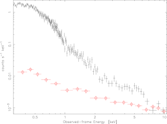
Figure 1: The pn source and background spectra. The upper curve (black crosses) is the source plus background spectrum. The lower curve (red, open circles) is the background spectrum. The data above 7.2 keV are ignored as the source spectrum becomes background dominated.

In addition, the MOS data were ignored below 0.7 keV due to the uncertainties in the low-energy redistribution characteristics of the cameras (Kirsch 2003). When fitted with a power-law, the MOS1 data above 2.5 keV displayed a steeper slope compared to the equivalent pn and MOS2 slopes ($\Delta\Gamma\sim$ 0.20–0.25). This inconsistency in the MOS1 data was previously realised in observations of 3C 273 by Molendi & Sembay (2003). Molendi & Sembay noted a difference in the MOS1 photon index compared to the other EPIC photon indices of $\Delta\Gamma$ $\sim$ 0.1. We note that since the PHL 1092 high-energy spectra are dominated by the pn data, and that the high-energy photon statistics are generally poor compared to the low-energy statistics, the inconsistency in the MOS1 photon index has little adverse effect on the results. All of the MOS data above 0.7 keV, and pn data above 0.3 keV were utilised during the spectral fitting, but the residuals from each instrument were examined separately to judge any inconsistency.

The source spectra were grouped such that each bin contained at least 20 counts. Spectral fitting was performed using XSPEC v11.2.0 (Arnaud 1996). Fit parameters are reported in the rest-frame of the object, although most of the figures remain in the observed-frame. The quoted errors on the model parameters correspond to a 90% confidence level for one interesting parameter (i.e. a $\Delta\chi^{2}$ = 2.7 criterion). Luminosities are derived assuming isotropic emission. The Galactic column density toward PHL 1092 is $N_{H}$ = (3.6 $\pm$ 0.2) $\times$ 10²⁰ cm^-2 (Murphy et al. 1996). A value for the Hubble constant of $H_{0}$=$\rm 70\ km\ s^{-1}\ Mpc^{-1}$ and a standard cosmology with $\Omega_{M}$ = 0.3 and $\Omega_{\Lambda}$ = 0.7 has been adopted.

3.1 The broad-band spectrum

A single absorbed power-law is a poor fit to the 0.3–7.2 keV data ($\chi^{2}$ = 870.5/266 $dof$). The high statistics below $\sim$ 2 keV dominate the fit resulting in large residuals at higher energies which demonstrates the need for multiple continuum components. For illustrative purposes, a single power-law ($\Gamma=$ 1.42${}^{+0.63}_{-0.50}$) modified by Galactic absorption was fitted to the 3–7.2 keV EPIC data and extrapolated to lower energies. The fit reveals the impressive strength of the soft-excess below $\sim$ 2 keV (Figure 2).

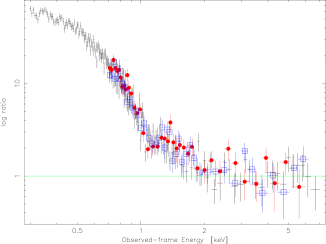
Figure 2: The ratio (data/model) resulting from fitting an absorbed power-law ($\Gamma=$ 1.42${}^{+0.63}_{-0.50}$) to the 3–7.2 keV EPIC data and extrapolating to lower energies. The black crosses, red dots, and blue squares correspond to the pn, MOS1, and MOS2 residuals, respectively. Note that the ratio axis is logarithmic.

Thermal disc models were implemented to fit the soft excess. Either a single blackbody or a multi-colour disc blackbody (MCD; Mitsuda et al. 1984; Makishima et al. 1986) would be a valuable supplement to the initial power-law fit ($\chi^{2}$ = 289.6/264 $dof$ and $\chi^{2}$ = 290.1/263 $dof$, respectively). The intrinsic column density was treated as a free parameter and determined to be insignificant in both models ($<$ 10¹⁹ cm^-2) A double power-law fit and a broken power-law fit were also attempted to assess whether the soft excess could be attributed to Comptonisation. Neither the double power-law nor the broken power-law models were statistically acceptable ($\chi^{2}$ = 480.0/263 $dof$ and 464.3/263 $dof$, respectively). In addition, both Comptonisation models required a high intrinsic column density, on the order of 10²¹ cm^-2. Such a large amount of intrinsic cold absorption above the Galactic value is inconsistent with the previous findings with $ROSAT$ (Forster & Halpern 1996; Lawrence et al. 1997; BBFR). The high column density derived with the power-law models is undoubtably manifested to accommodate a soft excess with intrinsic curvature.

Regardless of the prefered continuum model, a depression remained in the residuals at approximately 1 keV (1.4 keV in the rest-frame; Figure 3).

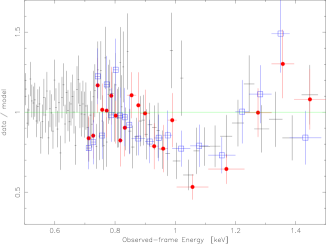
Figure 3: An absorption-like feature detected in all three EPIC instruments at $\sim$ 1 keV ($\sim$ 1.4 keV in the rest-frame). The continuum is represented by the best-fit model described in Sect. 3 and Fig. 5. See also model (a) in Table 2. The black crosses, red dots, and blue squares correspond to the pn, MOS1, and MOS2 residuals, respectively. The data have been re-binned for display purposes.

A Gaussian profile was added to the fits to model a potential absorption line. The supplementary component was an improvement to both the blackbody plus power-law fit ($\Delta\chi^{2}$ = 16.1 for the addition of 3 free parameters) and the MCD plus power-law fit ($\Delta\chi^{2}$ = 31.1 for the addition of 3 free parameters). The best-fit energy and equivalent width ($E=1.43\pm 0.04$; $EW=-82^{+19}_{-22}$) are consistent with similar features observed in other NLS1 (e.g. Leighly 1999b; Vaughan et al. 1999). The addition of a Gaussian profile was also a significant improvement to the Comptonisation models; however, it did not alleviate the requirement of a high column density in these models. Replacing the absorption line with an edge also improved the fit, but not as well as the line model ($\Delta\chi^{2}$ = 17.5 for the addition of 2 free parameters to the MCD plus power-law model). The edge energy is $E$ $\approx$ 1.33 keV, inconsistent with the strong edges arising in a warm absorber (e.g. O VII or O VIII). The residuals between about 1–1.2 keV in Figure 2 show a slight rise. We examined the possibility that the residuals in the 1–2 keV range could be due to an emission feature rather than absorption. Indeed an emission feature was an improvement to the MCD plus power-law fit ($\Delta\chi^{2}$ = 25.3 for the addition of 3 free parameters), but not quite as good as an absorption line. In addition, the energy and strength of the feature ($E\approx$ 1.97 keV and $EW\approx$ 350 eV) are difficult to reconcile with the current understanding of warm emission. Furthermore, residuals still remained at $\sim$ 1 keV, and when these residuals were modelled the parameters of the emission feature were no longer constrained.

3.2 Evidence for a reflection component

In a statistical sense the MCD and power-law model with an absorption line at $\sim$ 1.4 keV is a very good fit ($\chi^{2}$ = 259.0/260 $dof$). However, when the fit is examined in detail, the residuals indicated some curvature in the spectra above 2 keV (Figure 4).

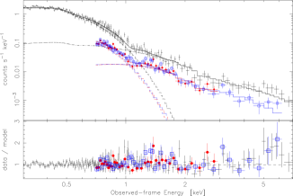
Figure 4: The MCD plus power-law and an absorption line model fitted to the EPIC 0.3–7.2 keV data (see text for details). In the lower panel the residuals (data/model) are show. While the fit is statistically acceptable, it is rather poor above $\sim$2 keV. The black crosses, red dots, and blue squares correspond to the pn, MOS1, and MOS2 points, respectively. For clarity the MOS1 data and residuals above 3 keV are not included in the figure (see text for detail).

Clearly, the degree of curvature observed at high energies will depend on how the soft continuum emission is modelled. Replacing the low-energy thermal component with a power-law did not eliminate the high-energy curvature. In addition, the quality of the fits were worse ($\chi^{2}_{\nu}>$ 1.1), and the models still required a high level of cold absorption.

Gradual flattening of the power-law toward higher energies has been observed in some other NLS1, and can be a quality attributed to a dominant reflection component (e.g. Fabian & Vaughan 2003) or partial-covering (Holt et al. 1980). While partial-covering has been relatively successful in describing the X-ray spectra of 1H 0707–495 (Boller et al. 2002) and IRAS 13224–3809 (Boller et al. 2003), the situation is more ambiguous in PHL 1092 due to the more modest statistics and the absence of a characteristic sharp spectral drop at energies above 7.1 keV (depending on the ionisation state of iron). We considered an absorption model by fitting the spectrum with a power-law plus edge. While the fit to the high-energy spectrum was good, the overall fit, including the soft X-ray components, was unacceptable ($\chi^{2}_{\nu}=$ 1.22).

A reflection dominated spectrum has also been suggested for 1H 0707–495 (Fabian et al. 2002) and IRAS 13224–3809 (Boller et al. 2003), as well as other NLS1 (Ballantyne et al. 2001). To test the reflection spectrum hypothesis a Gaussian profile was added to the fit to emulate an iron emission line. The improvement to the overall fit was significant ($\Delta\chi^{2}$ = 14 for the addition of 3 free parameters). The observed spectra can be described by a MCD plus power-law continuum, with warm absorption as well as a strong reflection component, all of which is modified by an amount of neutral absorption which is consistent with the Galactic column ($\chi^{2}$ = 245.0/257 $dof$; Figure 5; model (a) in Table 1). The temperature at the inner disc radius is 114 $\pm$ 4 eV. The power-law has a photon index of 2.55 $\pm$ 0.11. The absorption line is defined by $E$ = 1.43 $\pm$ 0.04 keV, $\sigma$ = 133${}^{+42}_{-37}$, and $EW$ = $-82^{+19}_{-22}$. The reflection component is modelled by a Gaussian profile with $E$ $\approx$ 6.9 keV, $\sigma$ $\approx$ 2 keV, and $EW$ $\approx$ 5 keV. Other models for the reflection component (e.g. diskline, laor, pexrav) were also effective in handling the high-energy curvature. In these cases the lines were slightly weaker ($EW=$ 2.5–4 keV); however, the quality of the data did not justify the use of these more complicated reflection models. The very strong iron lines suggested for this PHL 1092 observation seem unphysical, and we will address this issue in Section 5.4.

(1)

(2)

(3)

(4)

(5)

(6)

(7)

(8)

(9)

(10)

(11)

(12)

(13)

Model

$\chi^{2}_{\nu}$

NH

$kT$

$\Gamma_{1}$

$\Gamma_{2}$

$E_{brk}$

$E$

$\sigma$

$EW$

$E$

$\sigma$

$EW$

(dof)

(1020 cm-2)

(eV)

(keV)

(keV)

(eV)

(eV)

(keV)

(keV)

(keV)

(a)

0.95 (257)

$<$0.03

114$\pm$4

2.55$\pm$0.11

–

–

1.43$\pm$0.04

133${}^{+42}_{-37}$

$-82^{+19}_{-22}$

6.9

2

5

(b)

0.95 (258)

$<$0.03

112${}^{+2}_{-5}$

2.74${}^{+0.15}_{-0.11}$

1.49${}^{+0.28}_{-0.32}$

2.25${}^{+0.40}_{-0.31}$

1.43$\pm$0.04

144${}^{+41}_{-37}$

$-91^{+21}_{-22}$

–

–

–

(c)

1.07 (257)

6.6$\pm$0.2

–

4.64$\pm$0.12

1.80$\pm$0.26

1.88$\pm$0.11

1.28$\pm$0.06

300${}^{+33}_{-28}$

$-197^{+7}_{-5}$

7.2

0.71

0.52

Table 2: Spectral fits to the 0.3–7.2 keV (0.4–10 keV rest-frame) EPIC data. The two best-fits are models (a) MCD plus power-law continuum plus listed features, and (b) MCD plus broken power-law and listed features. Model (c) is the best-fit Comptonisation continuum model shown for comparison. Columns (4) to (7) are related to the continuum model: $kT$ is the thermal temperature at the innermost disc radius; $\Gamma_{1}$ and $\Gamma_{2}$ are the photon indices of the power-law components (two photon indices are required in the case of a broken power-law); $E_{brk}$ is the energy at which the photon index changes between $\Gamma_{1}$ and $\Gamma_{2}$ in the broken power-law model. Columns (8) to (10) are the absorption line components: line energy, width, and equivalent width ($E$, $\sigma$, $EW$, respectively), and columns (11) to (13) are the emission line components (best-fit values): line energy, width, and equivalent width ($E$, $\sigma$, $EW$, respectively). All models have been modified by line-of-sight Galactic absorption (3.6 $\times$ 10²⁰ cm^-2).

The average 0.3–7.2 keV unabsorbed flux is 1.91 $\times$ 10^-12 erg s^-1 cm^-2 (1.78 $\times$ 10^-12 erg s^-1 cm^-2 in the 0.3–2 keV band), corresponding to an observed luminosity of 8.8 $\times$ 10⁴⁴ erg s^-1. During the 18-day $ROSAT$ HRI monitoring campaign of PHL 1092, BBFR measured a 0.2–2 keV luminosity between 0.5–7.5 $\times$ 10⁴⁵ erg s^-1. Extrapolating our best-fit model from 0.3 keV to 0.2 keV, we estimate an average 0.2–2 keV luminosity of 1.1$\times$ 10⁴⁵ erg s^-1.

In comparison with the $ASCA$ luminosities reported by Vaughan et al. (1999; after correcting for the different cosmology which was assumed), we note that the intrinsic 0.6–10 keV luminosity is about 12% higher during the XMM-Newton observation. However, in the 0.6–2 keV band the XMM-Newton observation is $\approx$ 67% brighter, whereas the 2–10 keV luminosity is about 60% dimmer. The relative change in the various X-ray bands suggests long-term spectral variability in PHL 1092; however, the significance of this result cannot be tested without knowledge of the flux uncertainties in the $ASCA$ data.

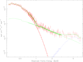
Figure 5: The unfolded model plotted to the EPIC pn data. The strong, broad emission line dominates the high-energy spectrum lending to the hypothesis that the spectrum is reflection dominated.

The broad-band continuum could be modelled equally well with a MCD plus a broken power-law above $\sim$ 2 keV ($\Gamma_{1}\approx$ 2.7, $\Gamma_{2}\approx$ 1.4, $E\approx$ 3.1 keV), and a $\sim$ 1.4 keV absorption line ($\chi^{2}$ = 245.4/258 $dof$). However, it is difficult to understand the physical significance of the high-energy break. Fit parameters for three of the best-fit models are shown in Table 2 for comparison. It is apparent from Table 2 that the low-energy spectrum is better fit with a blackbody component rather than a power-law.

3.3 The true soft-excess and the need for high-energy curvature

When fitting the 3–7.2 keV (4.2–10 keV rest-frame) spectrum and extrapolating downward in energy, as was done for Figure 2, there is evidence for an incredibly extreme soft-excess component, but no support for high-energy curvature. However, the need for high-energy curvature is seen when the broad-band spectrum is modelled in full. The simple power-law plus blackbody fit is significantly improved when a third component is introduced. Success is obtained when the simple continuum model is modified with either a strong, broad $\sim$ 2 keV Gaussian profile, or a high-energy break in the power-law, or a strong, broad iron fluorescence line. We attempt to demonstrate the curvature in the high-energy spectrum on a more basic level.

The 2.5–4 keV rest-frame data were fitted with a single absorbed power-law ($\Gamma\approx$ 2.6). While the photon index is steep compared to what is normally measured in AGN it is not atypical of NLS1-type objects (e.g. Brandt et al. 1997; Porquet et al. 2004). The 2.5–4 keV region was selected because it was the region most unlikely to have a significant contribution from the soft-excess or possible line emission, based on the general knowledge of AGN X-ray spectra.

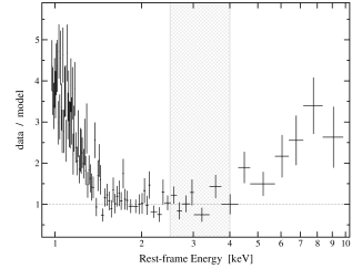
Figure 6: The residuals resulting from fitting the rest-frame 2.5–4 keV pn data (shaded region) with an absorbed power-law, and extrapolating to higher and lower energies. The data have been binned up for display purposes only. Note that the energy axis is given in the rest-frame.

The fit was then extrapolated to lower and higher energies as seen in Figure 6 (note the rest-frame energy axis). The extrapolation to higher energies is clearly poor indicating that there is a change in the spectral slope somewhere between 2.5–10 keV (rest-frame). The extrapolation to lower energies is quite reasonable down to 1.5 keV (rest-frame), at which point there is a rather dramatic upturn in the residual, likely marking the $true$ onset of the soft-excess. Pounds & Reeves (2002) examine the soft-excess in a small sample of Seyfert 1 galaxies. One of their conclusions is that the onset of the soft-excess is related to the 2–10 keV luminosity, such that in more luminous objects the soft-excess originates at higher energies. Comparing PHL 1092 to their sample (correcting for the different cosmology), we determined that a soft-excess starting at 1.5 keV (rest-frame) in PHL 1092 is precisely where the onset is expected.

4 Variability Properties

4.1 Extreme X-ray variability

Light curves from the two XMM-Newton observations of PHL 1092 are displayed in Figure 7; July 2000 on the left side, and January 2003 on the right (hereafter GT and AO2, respectively). The 0.3–1.4 keV (0.4–2 keV in the rest-frame) light curve during the GT observation shows periods of rapid flux drops and periods of relative quiescence. Overall, the X-ray intensity diminishes by nearly 70% during the 26 ks observation. During the AO2 observation the average count rate is about twice as high as during the GT observation. The 0.3–1.4 keV light curve again exhibits a diminishing intensity from the start of the observation to the end. However, during the second observation, the flux drop is more gradual. The peak intensity falls by about 50% over the first 23 ks.

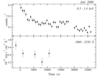
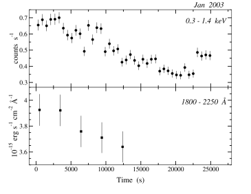
Figure 7: On the left side are the light curves corresponding to the July 2000 (GT) observation of PHL 1092. On the right side are the January 2003 (AO2) light curves. In the upper panels on both sides are displayed the variability in the 0.3–1.4 keV range ($\sim$ 0.4–2 keV in the rest-frame; 600 s bins). In the lower panels on both sides are the UVW2 light curves from each observation (1800–2250 Å observed-frame; $\sim$ 1290–1600 Å rest-frame; 2300 s exposures during GT, and 2640 s exposures during AO2).

The most rapid event during the AO2 observation occurs during the final 5 ks. After reaching a minimum intensity at about 23 ks, the flux suddenly rises by $\sim$ 30%, and remains there to the end of the exposure. Averaging over two low and two high data points in this event (1200 s on each side), the change in the rest-frame count rate is 0.12 counts s^-1 in 860 s. Adopting the average luminosity discussed in the previous section to determine a conversion factor between count rate and flux, we find that the event corresponds to a luminosity change of $\Delta$L = 2.0 $\times$ 10⁴⁴ erg s^-1. The luminosity rate of change is $\Delta$L/$\Delta$t $\approx$ 2.3 $\times$ 10⁴¹ erg s^-2. Quantifying this rate of luminosity change in terms of a radiative efficiency, $\eta>4.8\times 10^{-43}$$\Delta$L/$\Delta$t, (Fabian 1979), we calculate $\eta>0.11$. The measured value of $\eta$ is consistent with that expected from a Kerr black hole, but it exceeds the efficiency limit for a Schwarzschild black hole. While this is the most rapid event measured during this observation, BBFR found that, along with giant-amplitude flares, smaller amplitude flaring events were also rather common in PHL 1092, during periods of relative low flux (see Figure 1 of BBFR).

4.2 Simultaneous UV variability

An interesting discovery from this analysis is the simultaneous UV fluctuations of PHL 1092 which may be apparent at both epochs (Figure 7 lower panels). Fitting a constant to both UV light curves results in $\chi^{2}_{\nu}=$ 2.01 and 1.12 for the GT and AO2 observations, respectively; indicating variability at the $>$ 90% and $\sim$ 66% confidence levels. While not statistically significant, the UV light curves are short ($\sim$ 3 hours), not well-sampled, and of modest signal-to-noise (uncertainties on the level of 5%). Despite these observational constraints, variability trends are seen which appear consistent with the variability detected in the X-rays (more so during AO2). In addition, these short UV light curves are in contrast to what has been observed in the OM light curves of other NLS1 which normally show quite constant UV variability curves (e.g. Gallo et al. 2004a, 2004b). Unfortunately, relative photometry, to test the reliability of the UV light curves in Figure 7, is not possible due to the method in which the OM observation was carried out. As described by Mason et al. (2002), in the default OM imaging mode there are five exposures made up of two image windows each. While one window remains fixed on the central X-ray source during all five exposures (PHL 1092 in our case), the second window is moved across the CCD in order to maximize the field-of-view coverage. As a result, there is minimum overlap in the different windows, and no potential standard star is observed more than once.

Focusing on the AO2 observation, it may appear that the UV and X-rays are undergoing a gradual decline in flux during the first 13 ks. During this time the X-ray count rate drops by about 40%, whereas the UV flux drops by an average of 7% with an upper limit of 13% (not making any corrections for host galaxy and emission-line contamination). Without a longer base line on both light curves (and a higher signal-to-noise UV light curve) it is impossible to discuss how significant this result is, or if the two processes are physically connected (e.g. reprocessing, pivoting power-law, partial-covering).

There also appears to be long-term variability in the UV to X-ray spectral slope between the two epochs. In a rough approximation, utilising the values from the light curves, we see that the fraction of the mean X-ray count rate over the mean UV flux ($\div 10^{-15}$) has changed from 0.030 $\pm$ 0.001 during the GT observation, to 0.133 $\pm$ 0.002 during AO2. We examined whether the change in the UV flux is due to instrumental effects by making note of the UV fluxes of two other objects which were observed at both epochs (Table 3). One of these objects is a G5 star (HD 10214); hence its brightness should be rather stable over the $\sim$ 2 year period. As we see from Table 3 the UV flux in these comparison objects does change, and this could be associated with changes in the intrinsic luminosity of the sources or instrumental effects. However, the UV flux change in PHL 1092 is larger and opposite to that observed in the other two objects; hence the variability appears to be intrinsic to PHL 1092.

Object	Classification	GT Flux	AO2 Flux	Change
HD 10214	G5 star	307 $\pm$ 1	325 $\pm$ 1	$+6$%
UGC 00649	Sab galaxy	30.7 $\pm$ 0.3	33.2 $\pm$ 0.3	$+8$%
PHL 1092	AGN	4.43 $\pm$ 0.05	3.79 $\pm$ 0.05	$-14$%

Table 3: Long-term differences in the UV fluxes of identified OM sources. UVW2 flux densities are given in units of $\times$10^-15 erg s^-1 cm^-2 Å^-1.

A typical $\alpha_{ox}$ derivation is difficult to accomplish without making some assumptions about the UV spectral slope; hence it will not be calculated here.

In general, the variability is impressive for an object with an X-ray luminosity of $\sim$ 10⁴⁵ erg s^-1. Moreover, the rapid variability seems to extend to lower energies.

4.3 Spectral variability

Comparing the $ASCA$ and XMM-Newton observations there appears to be long-term X-ray spectral variability. Considering the OM and EPIC fluxes from the two XMM-Newton observations there also appears to be significant variability in the UV/X-ray spectral slope. However, examining short-term spectral variability within a single observation is difficult given the degree of high-energy background flaring during AO2. We search for flux related spectral variability, by constructing and comparing a high-flux spectrum and a low-flux spectrum. The high-flux state corresponded to all events with a count rate greater than 0.5 counts s^-1 in Figure 7 (right panel). This was roughly equivalent to selecting all events prior to $\sim$ 12 ks. The low-flux state was made up of all remaining events. In Figure 8 we have plotted the ratio between the high-flux and low-flux background-subtracted spectra. Note that the ratio spectrum only goes to $\sim$6.5 keV, as the low-flux spectrum is background dominated above this energy.

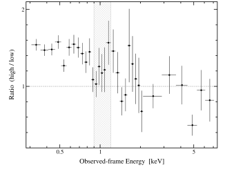
Figure 8: The EPIC pn background-subtracted ratio spectrum (high/low). To compare the spectrum to a constant a dotted-line is drawn in at high/low = 1. While the flux difference in the soft emission is remarkable, the variability above 2 keV is insignificant. The shaded region marks the approximate position of the $\sim$ 1.4 keV absorption feature based on Fig. 3.

For comparison to a constant, a line is drawn at a value of high/low = 1. The variability is obvious. At low-energies, $<$ 1 keV (1.4 keV rest-frame), the variability is remarkable, on the order of 50%. However, at energies above $\sim$ 1.4 keV (2 keV in the rest-frame), Figure 8 shows no indication of significant variability. Despite the extreme soft X-ray variability seen in Figure 7, it would seem that the hard X-rays are not particularly variable.

The shaded region in Fig. 8 marks the approximate position of the $\sim$ 1.4 keV absorption feature based on Fig. 3. Within the uncertainties, the variability in this region is weak, and most likely related to the underlying continuum rather than the absorption line itself.

5 Discussion

5.1 General findings

The main results of this study are listed below.

• The soft excess can be best-fit with a MCD (or blackbody) modified by Galactic absorption. An absorption feature was detected at $E\approx$ 1.4 keV ($EW\approx-$82 eV). The emission gradually flattens as the energy increases, introducing curvature to the high-energy ($>$ 2 keV) spectra. This curvature can be modelled empirically with a Gaussian profile ($E\approx$ 6.9 keV, $EW\approx$ 5 keV) or a broken power-law ($\Gamma_{1}\approx$ 2.7, $\Gamma_{2}\approx$ 1.4, $E\approx$ 3.1 keV in the rest-frame).

• Comparing the high-flux and low-flux spectra suggests significant short-term spectral variability. While the soft component is remarkably variable, the hard component shows no considerable variability. Long-term X-ray spectral variability is also suggested by a simple comparison between the $ASCA$ and XMM-Newton luminosities in different energy bands. In addition, long-term fluctuations in the X-ray/UV spectral slope are indicated by comparing the simultaneous UV and X-ray fluxes for each XMM-Newton observation.

• The UV and soft X-ray light curves from the two separate XMM-Newton observations show extraordinary short-term variability for such a luminous quasar ($\sim$ 10⁴⁵ erg s^-1). Radiative efficiency calculations during the AO2 observation exceed the limit for accretion onto a Schwarzschild black hole.

5.2 The $\sim$1.4 keV absorption feature

An absorption line at $\sim$ 1.4 keV has been detected in a number of NLS1 (e.g. Leighly 1999b; Vaughan et al. 1999; Boller et al. 2003). Leighly et al. (1997) examined the possibility that such features were O VII-O VIII edges, significantly blueshifted due to relativistic outflows. On the other hand, Nicastro et al. (1999) explain this type of absorption feature as a blend of resonant absorption lines, mainly due to Fe L, in a highly ionized warm absorber. A strong, steep, soft-excess is a requisite for the Nicastro et al. interpretation, which appears relevant in PHL 1092. To the best of our knowledge, PHL 1092 is the most luminous, NLS1 type object, in which possible Fe L absorption has been detected.

The absorption feature in PHL 1092 was not detected during the $ASCA$ observations. We simulated $ASCA$-SIS data by using the XMM-Newton model with the same number of counts that were obtained during the real $ASCA$ observation. In this case, the absorption line could have been detected, although it was not clearly seen in the residuals ($\Delta\chi^{2}\approx$ 16 for 3 additional free parameters). This could be indicative of long-term variability in the absorption feature, but we cannot dismiss the possibility of normalisation and/or profile changes in the low-energy continuum which will alter the apparent strength of any constant line features. However, since the ionising X-ray luminosity in PHL 1092 is so highly variable it is possible to consider that the strength of the $\sim$1.4 keV feature is also time variable.

As mentioned, during the $ASCA$ observations the total intrinsic 0.6–10 keV luminosity was about 10% lower than during the AO2 observation. Variability on this scale is typical for PHL 1092 in the course of hours. What may be more relevant here is the strength of the soft-excess component. During the $ASCA$ observations the soft-to-total intrinsic luminosity ratio ($l=L_{0.6-2~{}keV}/L_{0.6-10~{}keV}$) was $l_{ASCA}\approx 0.56$, where as during AO2 the ratio was $l_{AO2}=0.84\pm 0.04$ (uncertainties were not published for the $ASCA$ observation). The strength of the soft-excess could be an important consideration if the $\sim$ 1.4 keV feature is indeed variable in PHL 1092.

5.3 The rapid flux variability

The large-amplitude and rapid X-ray variability is impressive for a quasar of this luminosity, but more extreme behavior has been observed in this object before. It was during the $ROSAT$ HRI monitoring campaign that BBFR critically examined the underlying assumptions in the derivation of the radiative efficiency limit. The standard derivation assumes a uniform, spherical emission region with the release of radiation localized at its centre. It assumes that relativistic Doppler boosting and light bending are unimportant. Therefore, it is more than likely that the high and sometimes extreme values of the radiative efficiency measured in PHL 1092 are due to one or more of these standard assumptions being violated. The spectral properties discussed in Section 3, in particular the large equivalent width of the iron line, may suggest that light bending effects are considerable in this object (see also Section 5.4).

A new development, however, is the apparent simultaneous UV variability, and lack of hard X-ray variability. Without a high quality UV spectrum of PHL 1092, it is difficult to determine what could be the driving component responsible for the UV variability. Assuming that the UV spectrum of PHL 1092 is similar to that of I Zw 1 (Laor et al. 1997), another strong iron emitting NLS1, we can hypothesis that the source of the variability is continuum since line-emission is rather modest in this spectral region (1290–1600 Å intrinsic). Therefore, it is unlikely that the continuum variations are much stronger than those seen in Figure 7 (i.e. the continuum variability is probably not suppressed by line emission). Any models to be considered must, therefore allow for rapid, large-amplitude X-ray variability and weak UV variability. Currently, such models cannot be meaningfully discussed without longer base line and higher quality light curves.

5.4 Light Bending Model

A number of empirical models can been used to fit the high-energy curvature successfully, for example: a reflection-dominated spectrum, a high-energy broken power-law, or a broad 2 keV emission line in addition to the continuum. The problem with the latter two models is that they lack a clear physical interpretation. Recently, it was demonstrated how a spectrum could be reflection dominated via light bending effects (Martocchia, Karas, & Matt 2000; Fabian & Vaughan 2003; Miniutti et al. 2003; Miniutti & Fabian 2004). Uttley et al. (2003) consider a strong reflection component enhanced by light bending effects in describing the spectrum of the NLS1 NGC 4051 in its extended low-flux state.

The very strong iron line ($EW\approx$ 2.5–5 keV depending on the adopted model) suggested for this PHL 1092 observations seems highly unphysical, and in contrast to the general belief that the overall strength of the line diminishes with luminosity (e.g. Reeves & Turner 2000; but also see Porquet & Reeves 2003). However, the large equivalent width can be understood through light bending. Theoretical modelling by Dabrowski & Lasenby (2001) demonstrate that in a maximally rotating black hole, with the primary source located off the rotation axis, and the observer at an inclination of 60°, fluorescence line equivalent widths as high as $\sim$ 5.5 keV could be realised. Interestingly, Miniutti & Fabian (2004) show that the power-law component could be significantly more variable than the reflection component which could help explain the apparently constant high-energy X-ray emission in the presences of the highly variably low-energy X-ray emission. In addition, the high values that have been measured for the radiative efficiency in PHL 1092 on numerous occasions can also be understood if gravitational light bending effects are accounted for.

5.5 Alternatives to light bending

We have already discussed that high-energy curvature could be an indication for partial-covering. In addition, much of the long-term spectral variability could be explained in terms of partial-covering. However, a basic partial-covering model is simply not a good fit to the current spectral data and the data quality to not warrant the use of more advanced models.

With respect to the amazing variability it is natural to consider relativistic beaming due to jet emission. PHL 1092 is radio-quiet, and to the best of our knowledge, only detected in the sensitive NRAO VLA Sky Survey (NVSS; Condon et al. 1998) at 1.4 GHz at the 1 mJy level. Furthermore, the spectra at higher energies are not consistent with jet emission.

There are, of course, other possibilities that could produce some of the features observed in PHL 1092 (e.g. steep spectrum, extreme $\eta$, short-lived flares). For example, an intervening medium, such as: ions (e.g. Di Matteo et al. 1997), magnetic fields (e.g. Merloni & Fabian 2001), bulk motion of flaring material (Reynolds & Fabian 1997; Beloborodov 1999), or a combination could explain a number of the effects seen in PHL 1092 over the years.

6 Conclusions

PHL 1092 has been long known for its extreme variability and large luminosity. This most detailed X-ray observation to date revealed interesting spectral features which certainly warrant a deeper look. The complicated mixture of spectral and timing properties can be explained $simultaneously$ if we consider light bending effects. In addition, the possibly correlated soft X-ray/UV variability demonstrates the potential for fruitful variability and reverberation mapping studies of PHL 1092.

References

- [1] Arnaud, K. A. 1996, Astronomical Data Analysis Software and Systems V, eds. Jacoby G. and Barnes J., ASP Conf. Series, 101, 17
- [2] Ballantyne, D. R., Iwasawa, K., & Fabian, A. C. 2001, MNRAS, 323 506
- [3] Beloborodov A. M. 1999, ApJ, 510, 123
- [4] Bergeron, J. & Kunth, D. 1980, A&A, 85, L11
- [5] Bergeron, J. & Kunth, D. 1984, MNRAS, 207, 263
- [6] Boller, Th., Fabian, A. C., Sunyaev, et. al. 2002, MNRAS, 329, 1
- [7] Boller, Th., Tanaka, Y., Fabian, A., et. al. 2003, MNRAS, 343, 89
- [8] Brandt, W. N. 1996, PhD thesis, Univ. Cambridge
- [9] Brandt, W. N., Mathur, S., & Elvis, M. 1997, MNRAS, 285, 25
- [10] Brandt, W. N., Boller, Th., Fabian, A. C., & Ruszkowski, M. 1999, MNRAS, 303, L58 (BBFR)
- [11] Condon, J. J., Cotton, W. D., Greisen, E. W., et al. 1998, AJ, 115, 1693
- [12] Dabrowski, Y. & Lasenby, A. N 2001, MNRAS, 321, 605
- [13] Di Matteo T., Celotti A., & Fabian A. C. 1997, MNRAS, 291, 805
- [14] Fabian, A. C. & Vaughan, S. 2003, MNRAS, 340, 28
- [15] Fabian, A. C., Ballantyne, D. R., Merloni, A., et al. 2002, MNRAS, 331, 35
- [16] Fabian, A. C. 1979, Proc. R. Soc. London, Ser. A, 366, 449
- [17] Forster, K. & Halpern J. P. 1996, ApJ., 468, 565
- [18] Gallo, L. C., Boller, Th., Tanaka, Y., et al. 2004a, MNRAS, 347, 269
- [19] Gallo, L. C., Boller, Th., Brandt, W. N., et al. 2004b, A&A, 417, 29
- [20] den Herder, J. W., Brinkman, A. C., Kahn, S. M., et al. 2001, A&A, 365, 7
- [21] Holt, S. S., Mushotzky, R. F., Boldt, E. A., et al. 1980, ApJ, 241, 13
- [22] Jansen, F., Lumb, D., Altieri, B., et al. 2001, A&A, 365, 1
- [23] Kawaguchi, T., Mineshige, S., Umemura, M., & Turner, E. L. 1998, ApJ. 504, 671
- [24] Kirsch, M. 2003, XMM-Newton Calibration Presentations (CAL-TN-0018-2-1)
- [25] Laor, A., Jannuzi, B. T., Green, R. F., & Boroson, T. A. 1997, ApJ, 489, 656
- [26] Lawrence, A., Elvis, M., Wilkes, B. J., et al. 1997, MNRAS, 285, 879
- [27] Leighly, K. 1999a, ApJS, 125, 297
- [28] Leighly, K. 1999b, ApJS, 125, 317
- [29] Leighly, K. M., Mushotzky, R. F., Nandra, K., & Forster, K. 1997 ApJ., 489, 25
- [30] Makishima K., Maejima Y., Mitsuda K., et al., 1986, ApJ, 308, 635
- [31] Mason, K. O., Breeveld, A., Much, R., et al. 2001, A&A, 365, 36
- [32] Martocchia, A., Karas, V., & Matt, G. 2000, MNRAS, 312, 817
- [33] Merloni A. & Fabian, A. C. 2001, MNRAS, 321, 549
- [34] Miniutti, G., Fabian, A. C., Goyder, R., & Lasenby, A. N. 2003, MNRAS, 344, 22
- [35] Miniutti, G. & Fabian, A. C., 2004, MNRAS, 349, 1435
- [36] Mitsuda K., Inoue H., Koyama K., et al., 1984, PASJ, 36, 741
- [37] Molendi, S. & Sembay, S. 2003, XMM-Newton Calibration Presentations (CAL-TN-0036-1-0)
- [38] Murphy, E. M., Lockman, R. J., Laor, A., & Elvis, M. 1996, ApJS, 105, 369
- [39] Nandra, K., Le, T., George, I. M., et al. 2000, ApJ, 544, 734
- [40] Nicastro, F., Fiore, F., & Matt, G. 1999, ApJ, 517, 108
- [41] Porquet, D. & Reeves, J. N. 2003, A&A, 408, 119
- [42] Porquet, D., Reeves, J. N., O’Brien, P., & Brinkmann, W. 2004, accepted by A&A (astro/ph-0404385)
- [43] Pounds, K. A. & Reeves, J. N. 2002, (astro/ph-0201436)
- [44] Reeves, J. N. & Turner, M. J. L. 2000, MNRAS, 316, 234
- [45] Reynolds, C. & Fabian, A. 1997, MNRAS, 290, 1
- [46] Strüder, L. Briel U., Dennerl K., et al. 2001, A&A, 365 18
- [47] Turner, M. J. L., Abbey A., Arnaud M., et al. 2001, A&A, 365, 27
- [48] Uttley, P., Fruscione, A., McHardy, I., & Lamer, G. 2003, ApJ., 595, 656
- [49] Vaughan, S., Reeves, J., Warwick, R., Edelson, R. 1999, MNRAS, 309, 113