The Hubble Constant from gravitational lens CLASS B0218+357 using the Advanced Camera for Surveys

Abstract

We present deep optical observations of the gravitational lens system CLASS B0218+357 from which we derive an estimate for the Hubble Constant ($H_{0}$). Extensive radio observations using the VLA, MERLIN, the VLBA and VLBI have reduced the degeneracies between $H_{0}$ and the mass model parameters in this lens to one involving only the position of the radio-quiet lensing galaxy with respect to the lensed images. B0218+357 has an image separation of only 334 mas, so optical observations have, up until now, been unable to resolve the lens galaxy from the bright lensed images. Using the new Advanced Camera for Surveys, installed on the Hubble Space Telescope in 2002, we have obtained deep optical images of the lens system and surrounding field. These observations have allowed us to determine the separation between the lens galaxy centre and the brightest image, and so estimate $H_{0}$.

We find an optical galaxy position – and hence an $H_{0}$ value – that varies depending on our approach to the spiral arms in B0218+357. If the most prominent spiral arms are left unmasked, we find $H_{0}$ = 70$\pm$5 km s^-1 Mpc^-1(95% confidence). If the spiral arms are masked out we find $H_{0}$ = 61$\pm$7 km s^-1 Mpc^-1(95% confidence).

1 Introduction

Objects at cosmological redshifts may be multiply imaged by the action of the gravitational field of foreground galaxies. The first such example of gravitational lensing was the system 0957+561 (Walsh, Carswell & Weymann 1979) in which the core of a background quasar is split into two images 6″ apart. Since then approximately 70 cases of gravitational lensing by galaxies have been found.

Refsdal (1964) pointed out that such multiple-image gravitational lens systems could be used to measure the Hubble constant, if the background source was variable, by measuring time delays between variations of the lensed image and inferring the difference in path lengths between the corresponding ray paths. The combination of typical deflection angles of $\sim$1″ around galaxy-mass lens systems with typical cosmological distances implies time delays of the order of weeks, which are in principle readily measurable. Time delays have been measured for eleven gravitational lenses to date: CLASS B0218+357 (Biggs et al. 1999; Cohen et al. 2000), RXJ 0911.4+0551 (Hjorth et al. 2002), 0957+561 (Kundic et al. 1997; Oscoz et al. 2001), PG 1115+080 (Schechter et al. 1997) CLASS B1422+231 (Patnaik & Narasimha 2001), SBS 1520+530 (Burud et al. 2002a), CLASS B1600+434 (Koopmans et al. 2000; Burud et al. 2002b), CLASS B1608+656 (Fassnacht et al. 1999; Fassnacht et al. 2002), PKS 1830$-$211 (Lovell et al. 1998), HE 2149$-$2745 (Burud et al. 2002b) and HE 1104$-$1805 (Ofek & Maoz 2003). In principle, given a suitable variable source, the accuracy of the time delay obtained can be better than 5%. This has already been achieved in some cases (eg. 0957+561) and there is no doubt that diligent future campaigns will further improve accuracy and also produce time delays for more gravitational lens systems.

Gravitational lenses provide an excellent prospect of a one-step determination of $H_{0}$ on cosmological scales. The major problem is that, in addition to the time delay, a mass model for the lensing galaxy is required in order to determine the shape of the gravitational potential. The model is needed to convert the time delays into angular diameter distances for the lens and source. In double-image lens systems in which the individual images are unresolved this is a serious problem as the number of constraints on the mass model (lensed image positions and fluxes) allows no degrees of freedom after the most basic parameters characteristic of the system (source position and flux together with galaxy mass, ellipticity and position angle) have been fitted. In four-image systems the extra constraints provide assistance, and in a few cases, such as the ten-image lens system CLASS B1933+503 (Sykes et al. 1998) more detailed constraints on the galaxy mass model are exploited (Cohn et al. 2001).

There are two further systematic and potentially very serious problems. The first is that the radial mass profile of the lens is almost completely degenerate with the time delay, and hence $H_{0}$ (Gorenstein, Shapiro & Falco 1988; Witt, Mao & Keeton 2000; Kochanek 2002). Given a time delay, $H_{0}$ scales as $2-\beta$, where $\beta$ is the profile index of the potential, $\phi\propto r^{\beta}$. Work by Koopmans & Treu (2003) shows that mass profiles may vary from an isothermal slope by up to 10% for single galaxies, producing corresponding uncertainties in $H_{0}$. The problem is particularly serious for four-image systems, because the images are all approximately the same distance from the centre of the lens and thus constrain the radial profile of the lensing potential poorly. On the other hand, for CLASS B1933+503, with three sources producing ten images, the radial mass profile is well constrained (Cohn et al. 2001). Unfortunately B1933+503 does not show radio variability (Biggs et al. 2000) and is optically so faint that measuring a time delay is likely to be very hard.

In some cases Einstein rings may provide enough constraints, despite the necessity to model the extended source which produces them (Kochanek, Keeton & McLeod 2001) although models constrained by rings may still be degenerate in $H_{0}$ (Saha & Williams 2001).

The mass profile degeneracy is particularly sharply illustrated by “non-parametric” modelling of lens galaxies (Williams & Saha 2000; Saha & Williams 2001). Such models assume only basic physical constraints on the galaxy mass profile, such as a monotonic decrease in surface density with radius. They find consistency with the observed image data for a wide range of galaxy mass models, which are themselves consistent with a wide range of $H_{0}$. Combining two well-constrained cases of lenses with a measured time delay, CLASS B1608+656 and PG 1115+080, Williams & Saha (2000) find H${}_{0}=61\pm 18$km s^-1 Mpc^-1(90% confidence).

There are a number of approaches to the resolution of the mass profile degeneracy problem. One is to assume that galaxies have approximately isothermal mass distributions. ($\beta\sim 1$). There are two parts to the lensing argument in favour of isothermal galaxies: from the lack of odd images near the centre of observed lens systems Rusin & Ma (2001) are able to reject the hypothesis that significant number of lensing galaxies have profiles which are much shallower ($\beta>1.2$) than isothermal, assuming a single power-law model is appropriate for the mass contained interior to the lensed images. Similarly it can be shown that models which are significantly steeper than isothermal are unable to reproduce constraints from positions and fluxes in existing lenses with large numbers of constraints (e.g. Muñoz, Kochanek & Keeton 2001; Cohn et al. 2001). The most straightforward approach, that of assuming an isothermal lens, has been taken by many authors. In most cases this yields $H_{0}$ estimates of between 55 and 70 km s^-1 Mpc^-1 (e.g. Biggs et al. 1999; Koopmans & Fassnacht 1999; Koopmans et al. 2000; Fassnacht et al. 1999) but studies of some lenses imply much lower values (e.g. Schechter et al. 1997; Barkana 1997; Kochanek 2003). In fact, Kochanek (2003) finds a serious discrepancy with the HST key project value of $H_{0}$=71km s^-1 Mpc^-1 (Mould et al. 2000; Freedman et al. 2001) unless, far from being isothermal, galaxy mass profiles follow the light distribution.

Falco, Gorenstein & Shapiro (1985) pointed out the second important problem. Any nearby cluster produces a contribution to the lensing potential in the form of a convergence which is highly degenerate with the overall scale of the lensing system and hence with $H_{0}$. Unfortunately, the systems with the most accurately determined time delays and the best-known galaxy positions are often those with large angular separation such as 0957+561, and these are the systems in which lensing is most likely to be assisted by a cluster. Again progress can be made by appropriate modelling of the cluster, and many attempts have been made to do this for 0957+561 (e.g. Kundic et al. 1997; Bernstein & Fischer 1999; Barkana et al. 1999) although there remain uncertainties in the final $H_{0}$ estimate. As an alternative, the optical/infra-red images of the host galaxy may make an important contribution towards the breaking of degeneracies (Keeton et al. 2000).

Kochanek & Schechter (2004) summarise the contribution of lensing to the $H_{0}$ debate so far and present options for further progress. One approach is simply to accumulate more $H_{0}$ determinations and rely on statistical arguments to iron out the peculiarities which affect each individual lens system; this approach is vulnerable only to a systematically incorrect understanding of galaxy mass profiles. The alternative approach is to select a lens system in which additional observational effort is most capable of decreasing the systematic errors on the $H_{0}$ estimate to acceptable levels. In this paper we argue that CLASS B0218+357 is the best candidate for this process. We describe new Hubble Space Telescope (HST) observations using the Advanced Camera for Surveys (ACS) which are aimed at removing the last major source of systematic uncertainty in this system. We then describe how we use the imaging data to derive a value for the Hubble constant.

2 CLASS B0218+357 as a key object in $H_{0}$ determination

CLASS B0218+357 was discovered during the early phase of the CLASS survey, the Jodrell Bank-VLA Astrometric Survey (JVAS; Patnaik et al. 1992). B0218+357 consists of two images (A and B) of a background flat-spectrum radio source separated by 0$\aas@@fstack{\prime\prime}$334, together with an Einstein ring (Patnaik et al. 1993). The optical spectrum shows a red continuum source superimposed on a galaxy spectrum. The redshift of the lensing galaxy has been measured optically by Browne et al. (1993) and Stickel & Kuehr (1993), and by Carilli, Rupen & Yanny (1993) at radio wavelengths giving the most accurate result of 0.6847. Cohen et al. (2003) have measured the source redshift of 0.944.

It quickly became apparent that the lensing was performed by a spiral galaxy. Spiral lenses generally produce smaller image separations than elliptical lenses because of their lower mass. The spiral nature of B0218+357 was deduced directly from early high-resolution optical images from the Nordic Optical Telescope (Grundahl & Hjorth 1995), and was consistent with evidence from molecular line studies which revealed absorption of the radio emission from the background radio source by species in the lensing galaxy including CO, HCO⁺, HCN (Wiklind & Combes 1995), formaldehyde (Menten & Reid 1996) and water (Combes & Wiklind 1997). Moreover, in the optical, the A image, which is further from the galaxy, is fainter than the B image (Grundahl & Hjorth 1995) , despite being a factor $\sim$3 brighter in the radio. This suggests that the line of sight to the A image intercepts a great deal of dust, possibly associated with a giant molecular cloud in the galaxy. The lensing galaxy appears close to face-on, a conclusion deduced from its symmetrical appearance in optical images. This conclusion is consistent with the small velocity line-width of the absorption lines (e.g. Wiklind & Combes 1995).

Further radio imaging resolved both the A and B images into core-jet structures (Patnaik, Porcas & Browne 1995; Kemball et al. 2001; Biggs et al. 2003), as well as revealing more details of the Einstein ring (Biggs et al. 2001). The combined constraints from the core-jet structure and the ring together strongly constrain mass models. A and B lie at different distances from the galaxy, and with the Einstein ring constraints permits determination of both the angular structure of the lensing mass (Wucknitz et al. 2004) and (most importantly) the mass–radius relation for the lens.

Biggs et al. (1999) have determined a time delay of 10.5$\pm$0.4 days (95% confidence) for B0218+357 using radio monitoring observations made with the VLA at both 8.4 GHz and 15 GHz. Consistent results were obtained from the variations in the total intensity, the percentage polarization and the polarization position angle. Biggs et al. used the time delay and existing lens model to deduce a value for the Hubble constant of 69${}^{+13}_{-19}$ km s^-1 Mpc^-1(95% confidence). It should be noted, however, that the error bars on the assumed position for the lensing galaxy with respect to the lensed images were over-optimistic and hence their quoted error on $H_{0}$ is too small. Cohen et al. (2000) also observed B0218+357 with the VLA, and measured a value for the time delay of 10.1${}^{+1.5}_{-1.6}$ days. This corresponds to an $H_{0}$ value of 71${}^{+17}_{-21}$ km s^-1 Mpc^-1(95% confidence), the larger error bars in Cohen et al.’s measurement being due to their use of a more general model for the source variability, although they used the same model for the lensing effect as Biggs et al. The error bars do not take into account any systematic error associated with the uncertain galaxy position.

Lehár et al. (2000) used the then existing constraints to model the CLASS B0218+357 system. They found that, even for isothermal models, the implied value of $H_{0}$ was degenerate with the position of the centre of the lensing galaxy, with a change of about 0.7 km s^-1 Mpc^-1(about 1 per cent) in the value of $H_{0}$ for every 1 mas shift in the central galaxy position. Their uncertainty on the position derived from HST infra-red observations using the NICMOS camera is approximately $\pm$30 mas.

Recently, using a modified version of the LensClean algorithm (Kochanek & Narayan 1992; Ellithorpe et al. 1996; Wucknitz 2004), Wucknitz et al. (2004) have been able to constrain the lens position from radio data of the Einstein ring. With the time delay from Biggs et al. (1999) of $(10.5\pm 0.4)$ days, they obtain for isothermal models a value of H${}_{0}=78\pm 6$ km s^-1 Mpc^-1(95% confidence). They use VLBI results from other authors (Patnaik et al. 1995, Kemball et al. 2001) as well as their own data (Biggs et al. 2003) to constrain the radial profile from the image substructure and obtain $\beta\approx 1.04$, very close to isothermal ($\beta=1$). Our aim in this paper is to use new optical observations to determine the lensing galaxy position directly and to compare this with the indirect determination of Wucknitz et al. (2004).

We briefly summarise the reasons why, given the observations presented here, CLASS B0218+357 offers the prospect of the most unbiased and accurate estimate of $H_{0}$ to date.

1. The observational constraints are arguably the best available for any lens system with a measured time-delay.

2. The radio source is relatively bright (a few hundred mJy at GHz frequencies) and variable at radio frequencies, so time delay monitoring is relatively straightforward and gives a small error (Biggs et al. 1999) which can be improved with future observations.

3. The system is at relatively low redshift. This means that the derived values for $H_{0}$ will not depend on the matter density parameter and cosmological constant by more than a few percent.

4. The lens is an isolated single galaxy and there are no field galaxies nearby to contribute to the lensing potential (Lehár et al., 2000).

Although most lenses have at least one of these desirable properties, CLASS B0218+357 is the only one known so far which has all of them. It thus becomes a key object for $H_{0}$ determination. It is only the lack of an accurate galaxy position that led in the past to it being excluded from consideration by many authors (e.g. Schechter 2001; Kochanek 2003).

3 The ACS observations

Resolving the lens galaxy and lensed images is an aim that benefits from high resolution combined with high dynamic range, and so we asked for and were awarded time on the Advanced Camera for Surveys (ACS; Clampin et al. 2000) on the Hubble Space Telescope.

Although observations in the blue end of the spectrum would have maximised angular resolution, the likely morphological type of the lensing galaxy (Sa/Sab) meant that asymmetry due to star formation in the spiral arms could have caused problems in the deconvolution process which relies on symmetry in the lensing galaxy (see Section 5). Hence observations at wavelengths longer than 4000Å in the rest frame of the galaxy were desirable. At the redshift of the lens this dictated the use of I band, i.e. the F814W filter on the HST.

The ACS has two optical/near-IR “channels”, the Wide Field Channel (WFC) and the High Resolution Channel (HRC). The HRC’s pixel response exhibits a diffuse halo at longer wavelengths due to scattering within the CCD. As a result, roughly 10% of the flux from a point source will be scattered into this halo at 8000Å, possibly making it more difficult to resolve the lensing galaxy from the lensed images. We selected the WFC for use in our observing programme since it does not suffer from this effect. Unlike the HRC, the WFC moderately under-samples the HST point-spread function (PSF) at 8000Å. To counter this effect, we selected two distinct four-point dither patterns, alternating between them over the course of the observations. The dither patterns used are shown in Figure 1 (see also Mutchler & Cox 2001 for more information on HST dither patterns).

Figure 1: 4+4 dither pattern used for the observations of 0218+357. The pattern provides steps to the level of $\frac{1}{4}$-pixel.

The WFC has a field of view of 202″$\times$202″, and a plate scale of approximately 50 mas pixel^-1. Since we used a gain of unity, saturation in the images occurs near the 16-bit analogue to digital conversion limit of 65,000 e^- pixel^-1 rather than at the WFC’s full well point of 85,000 e^- pixel^-1. We determined the exposure time required on B0218+357 through simulation.

The full programme of B0218+357 observations was carried out over the period from August 2002 to March 2003. Details of the observing dates and exposure times are shown in Table 1. The total available telescope time was split into 7 visits on B0218+357, 6 of which provided 2 hours integration time on the science target. The remaining visit (16) was designed to permit the programme to be salvaged in the unlikely case that the observing pattern chosen for visits 10-15 proved to be both inappropriate and uncorrectable. This visit suffered from increased observing overheads relative to the other visits and provided an integration time of 1 hour, 22 minutes on B0218+357 as a result. In order to deconvolve the images we required an ACS/WFC PSF, so two short visits (1 and 2 in Table 1) were dedicated to observing two Landolt standard stars (Landolt 1992). Following McLure et al. (1999), observations were taken with several different exposure times to allow the construction of a composite PSF that would have good signal-to-noise in both core and wings whilst avoiding saturation of the core. Standards were selected to be faint enough not to saturate the WFC chip on short integration times, and to have the same $V-I$ colour, to within 0.2 magnitudes, as the lensed images in the B0218+357 system. The exposure times on the standard stars ranged from 0.5 seconds to 100 seconds each, the longest exposures each being split into two 50 second exposures to simplify cosmic ray rejection.

Visit no.	Target	Observation date	Exposure time	Dither pattern	File name root
10	CLASS B0218+357	2003 February 28	20$\times$360 sec	4+4	j8d410
11	CLASS B0218+357	2003 March 01	20$\times$360 sec	4+4	j8d411
12	CLASS B0218+357	2003 January 17-18	20$\times$360 sec	4+4	j8d412
13	CLASS B0218+357	2003 March 06	20$\times$360 sec	4+4	j8d413
15	CLASS B0218+357	2003 March 11	20$\times$360 sec	4+4	j8d415
14	CLASS B0218+357	2002 October 26-27	20$\times$360 sec	4+4	j8d414
16	CLASS B0218+357	2002 September 11	12$\times$360 sec	4+4	j8d416
			8$\times$75 sec	4C
1	92 245	2002 October 17-18	8$\times$0.5 sec	4+4	j8d401
			8$\times$8 sec	4+4
			1$\times$360 sec	-
2	PG0231+051B	2002 August 25	8$\times$0.5 sec	4+4	j8d402
			8$\times$8 sec	4+4
			8$\times$50 sec	4C

Table 1: Log of HST observations. All observations were taken with the ACS using the F814W filter, corresponding to I band. A 4+4 dither pattern refers to an eight-point dither consisting of two nested parallelograms, whereas 4C refers to a four-point dither parallelogram with the exposure at each point split into two for explicit cosmic-ray rejection.

4 Reduction of the ACS data

The uncalibrated data produced by automatic processing of raw HST telemetry files by the OPUS pipeline at the Space Telescope Science Institute (STScI) were retrieved along with flat fields, superdarks and other calibration files.

The data were processed through the ACS calibration pipeline, CALACS (Pavlovsky et al. 2002), which runs under NOAO’s IRAF software. The CALACS pipeline de-biased, dark-subtracted and flat-fielded the data, producing a series of calibrated exposures. The pipeline also combined the CR-SPLIT exposures in visits 1, 2 and 16 to eliminate cosmic rays. The calibrated exposures were in general of acceptable quality for use in the next stage of reduction, except for visit 15 in which there was some contamination of the images by stray light, probably from a WFPC2 calibration lamp (R. Gilliland and M. Sirianni, private communication). It is possible that this defect can be corrected in the future using the techniques which were used by Williams et al. (1996) to remove stray light from some HDF exposures, but we have not attempted to deconvolve the contaminated visit.

The calibrated exposures were fed to the next stage of reduction, based around the dither package (Fruchter & Hook 2002), and the STSDAS packages pydrizzle (Hack 2002) and multidrizzle (Koekemoer et al. 2002). These tools clean cosmic rays, remove the ACS geometric distortion and “drizzle” the data on to a common output image (Fruchter & Hook 2002). The drizzle method projects the input images on to a finer grid of output pixels. Flux from each input pixel is distributed to output pixels according to the degree of overlap between the input pixel and each output pixel. To successfully combine dithered images into a single output image, knowledge of the pointing offsets between exposures is needed. The expected offsets are determined by the dither pattern used, but the true offsets might vary from those expected due to thermal effects (Mack et al. 2003) within single visits. To determine the true pointing offsets between dithered exposures, we cross-correlated the images. Since the WFC at I-band moderately undersamples the HST’s PSF, and since most of the features detected in the images were extended rather than stellar, we opted for pixel-by-pixel cross-correlation rather than comparisons of positions of stars between different pointings, to maximise our use of the available information.

Images in each visit were drizzled on to a common distortion-corrected frame and then pairs of these images were cross-correlated. The two-dimensional cross-correlations have a Gaussian shape near their centres. The shift between pairs of images is measured by fitting a Gaussian function to the peak in the cross-correlation, and the estimated random error in the shift is derived from the position error given by the Gaussian fit. For our data, the random errors in the measured shifts ranged from 0.8 to 2.5 mas. The RMS scatter between corresponding pointings within a visit was typically less than 10 mas, or 20% of a single WFC pixel. We fed these shifts to the multidrizzle script, which carried out the drizzling of visits to common, undistorted output frames. As part of the drizzling process, we opted to decrease the output pixel size from 50 mas square (the natural size of the undistorted output pixels) to 25 mas square. To avoid blurring and “holes” in the output image, the input pixels were shrunk to 70% of their nominal size before being drizzled on to the output frames (Fruchter & Hook 2002). We used a gaussian drizzling kernel to slightly improve resolution and reduce blurring. At the end of this process each visit, except for visit 15, provided us with a output image with improved sampling compared to the individual input exposures. The deconvolution of these images is described in Section 5.

Since deconvolution depends greatly on the accuracy of the PSF model, we have produced a number of different PSFs. Unfortunately the Landolt standard star (Landolt 92 245) observed in visit 1 was resolved into a 0.5″ double by the ACS/WFC, so we have concentrated on extracting a PSF from visit 2 (Landolt PG0231+051B). The calibrated exposures were combined using multidrizzle. Saturated pixels were masked. The resulting PSF suffered from serious artifacts consisting of extended wings approximately 80 mas up and down the chip from the central peak, possibly due to imperfect removal and combination of pixels which were affected by bleeding of saturated columns. We believe these extended wings to be artifacts since they rotate with the telescope rather than the sky, and are not present in stars in other visits.

In lieu of ideal standard star PSFs, we have created per-visit PSFs by averaging field stars together. These field star PSFs do not suffer from the artifacts present in the visit 2 PSF. Manual examination, pixel-by-pixel, of the difference between the PSFs and the central regions close to image B, indicate that the RMS error in the PSFs is between 5 and 15%. Such an error increases linearly with the counts, rather than with their square root; lacking a perfectly-fitting PSF, we have allowed for this error when performing the data analysis described in Section 5.

5 Analysis of the position data and results

5.1 General remarks

Figure 2 shows the ACS image of the CLASS B0218+357 system from the combined dataset, consisting of all science visits on B0218+357 excluding visit 15. To produce this combined image, separate visits were related through restricted linear transformations (rotation and translation) based on the positions of unsaturated stars common to all images, and then co-added. In locating the lensing galaxy, however, we did not use this combined image, preferring to work with the separate visits. The two compact images (A and B) can be distinguished as can the lensing galaxy which lies close to B. The spiral arms of the galaxy are clearly seen confirming the earlier deductions that the lensing galaxy is a spiral (Wiklind & Combes 1995; Carilli et al. 1993). The spiral arms appear to be smooth and regular and there is no sign of significant clumping associated with large-scale star formation. The galaxy appears almost exactly face-on. We deduce this by assuming a galaxy position close to B and comparing counts between pixels at 90 degree angles from each other about the assumed centre. Examination of the residuals reveals no sign of ellipticity.

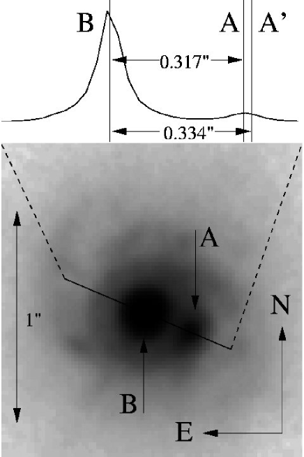
Figure 2: Combined ACS image of B0218+357. The lensed images are both visible; the brighter image, B, is close to the centre of the lensing galaxy. The spiral arms of the galaxy are clearly visible. The plot above the image shows a one dimensional slice passing through images A and B. The best-fit positions of A and B on this slice are marked, along with A’, the position of A expected from the radio image separation (334 mas). The separation between A and B in the optical image is 317$\pm$4 mas ($2\,\sigma$).

The core of the lensing galaxy is strongly blended with B (Figure 2) and is relatively weak. Extrapolation of an exponential disk fit to the outer isophotes of a slice through the central region shows that the peak surface brightness of image B exceeds that of the galaxy by a factor of about 30-50. Thus the determination of an accurate position for the galaxy is a challenging task. Before discussing the process in more detail below, we outline the various steps we go through to obtain a galaxy position. They are:

1. For each visit we measure the positions of the A and B images.

2. We subtract PSFs from these positions.

3. Using PSF-subtracted data we look for the galaxy position about which the residuals left after PSF subtraction appear most symmetric. We do not subtract a galaxy model from the images. This approach finds the centre of the most symmetric galaxy consistent with the data.

4. We compute the mean and variance of the galaxy positions found from the individual visits.

5.2 Analysis procedure

Our reduced ACS/WFC images are over 8450x8500 pixels in size, and cover 202″x202″on the sky. We cut out a region of 128x128 pixels (3.2″x3.2″) centred on the lens and analyse this to make fitting computationally practical and to isolate the lens from other objects on the sky.

Since the images, particularly image B, have much higher surface brightnesses than the galaxy, their positions can be located relatively accurately by subtracting parametric or empirical PSFs from the data and minimising the residuals. Fits were carried out on circular regions centred on the brightest pixel of each compact image. The regions chosen were 11 pixels in diameter. To avoid any bias arising from the choice of PSF, we used both parametric models (Airy and Gaussian functions) and the field star PSFs in the fits. The field star PSFs were consistently better fits to both A and B than the parametric models, Gaussians being insufficiently peaked and Airy functions having diffraction rings that were too prominent. A linear sloping background was modelled along with the PSF in order to take account of the flux due to the galaxy. Typically the various methods agreed on positions to within a tenth of a pixel (2.5 mas).

The separation of A and B determined by optical PSF fitting is consistently less than the radio separation of 334 mas. We find that the mean image separation in the optical is 317$\pm$2 mas (1$\,\sigma$) when the field star PSFs are used, and 315$\pm$4 mas when Gaussian PSFs are used. The corresponding result for Airy function PSFs is 311$\pm$10 mas. These values are mean separations taken over the six processed visits on B0218+357. We have checked the plate scale of drizzled images against stars listed in the US Naval Observatory’s B1.0 catalogue, and find that the nominal drizzled plate scale of 25 mas pixel^-1 is correct to better than 1% for all visit images.

An anomalous optical image separation has been suggested before for B0218+357, starting with ground-based optical imaging by Grundahl & Hjorth (1995) and again by Hjorth (1997). Jackson, Xanthopoulos & Browne (2000) used NICMOS imaging to find an image separation of 318$\pm$5 mas, in agreement with our result from field star PSFs.

We hypothesise that that this low separation may be a result of the high, and possibly spatially variable, extinction in the region of A. We suggest that some of the image A optical emission arises from the host galaxy rather than from the AGN which dominates the B image emission. Thus the centroid of A may not be coincident with the AGN image. Image A may be obscured completely and the emission seen could be due to a large region of star formation associated with an obscuring giant molecular cloud. In view of this possibility and the fact that B is consistently much brighter than A in the optical, we measure galaxy positions as offsets from our measured position for B. Thus, although A’s position may be distorted in the optical it does not directly influence our measurements of $H_{0}$.

Having determined positions and fluxes for A and B, we created an image containing two PSFs as a model for the flux from the lensed images alone (the “model image”). A model image was made separately for each visit and subtracted from each observed image, leaving a residual image which contained only the galaxy plus subtraction errors. Figure 3 shows a typical image with A and B subtracted. The model allowed us to keep track of how much PSF flux was removed from each pixel in producing the residual images.

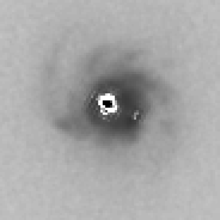
Figure 3: A visit image with A and B subtracted after fitting fluxes and positions. The residuals near the centre of each subtracted image show maxima of approximately 20% of the unsubtracted light.

We opted to use the criterion of maximum symmetry in the residuals as a goodness-of-fit parameter rather than attempting to fit a parametric model, such as an exponential disk profile, to the light distribution of the galaxy. The symmetry fit statistic is expressed as

$$\chi^{2}=\sum_{P}\frac{{\left|s({\bf r})-s({\bf r}^{\prime})\right|}^{2}}{\sigma({\bf r})^{2}+\sigma({\bf r}^{\prime})^{2}},$$ (1)

in which $s({\bf r})$ is the count-rate at image pixel position ${\bf r}=(x,y)$ in counts per second, $\sigma({\bf r})$ is the estimated noise at ${\bf r}$, $P$ is the set of pixels included in the fit (see below) and ${\bf r}^{\prime}$ is the reflection of ${\bf r}$ around the galaxy position ${\bf g}$, given by simple geometric considerations as

$${\bf r}^{\prime}=2{\bf g}-{\bf r}.$$ (2)

The random error for each pixel in the image, $\sigma({\bf r})$ is estimated from the CCD equation (Merline & Howell 1995) summed with a contribution from the assumed random error in the PSF. The estimate of the noise is given by

$$\sigma({\bf r})^{2}=\frac{q^{4}}{\tau^{2}}\frac{q^{-2}\tau s({\bf r})+S+R^{2}}{N}+\mu^{2}s_{p}({\bf r})^{2},$$ (3)

where $\tau$ is the integration time at a single dithered pointing, $\mu$ is the assumed fractional error in the PSF, $s_{p}({\bf r})$ is the count-rate from A and B alone (stored in the model image), $q$ is the drizzling scale factor (the ratio between output and input pixel size, 0.5 for these images) $N$ is the number of dithered pointings combined in the drizzle process, $S$ is the sky noise and $R$ is the ACS/WFC read noise. Both sky noise and read noise are expressed in units of electrons, and the integration time is in seconds. The resulting noise figure has units of counts per second, as does the drizzled image. We have checked this noise estimate against the background noise in our images and against simulations of the drizzling process.

The set of pixels (P) included in the calculation of this $\chi^{2}$ figure can bias the fit if it is ill-chosen. When ${\bf r}^{\prime}$ falls outside the boundaries of the image, the pixel ${\bf r}$ is considered to contribute nothing to the $\chi^{2}$ statistic and the pixel is not included in the set P. Such pixels therefore do not contribute to the number of constraints available and as a result do not increase the number of degrees of freedom in the fit. Alternative treatments can introduce bias; for instance, if these pixels are assigned large $\chi^{2}$ values the fitting program is biased towards placing the galaxy in the geometrical centre of the image. If the same pixels are considered to contribute zero towards the $\chi^{2}$ statistic but are still counted as part of the set P, they increase the number of degrees of freedom in the fit and bias the fit to positions away from the image’s geometrical centre. To avoid these possibilities we do not count degrees of freedom from pixels whose reflection about the galaxy centre ends up outside the image boundaries.

The symmetry criterion is non-parametric and has the advantage of minimizing the assumptions that are imposed on the data; the use of a particular distribution as a function of radius in any case contains an implicit assumption of symmetry. Using the symmetry criterion on its own is in principle robust whether or not the galaxy has a central bulge, and should also be unaffected if the galaxy contains a bar. The symmetry criterion will also hold for galaxies having moderate inclinations to the line of sight. For a circularly symmetric galaxy, the main effect of a small deviation away from a face-on orientation will be to render the observed image slightly elliptical. The basic symmetry criterion is that points and their reflections about the true centre of the galaxy’s image should have the same flux (to within the measurement errors). Therefore whether the galaxy’s image has circular or slightly elliptical isophotes is unimportant because in both cases the same isophote passes through both point and reflection. This argument breaks down for spirals with significant inclinations as absorption is likely to become important and destroy any symmetry present in the image.

The centre of maximum symmetry could be displaced by spiral arms if they are not themselves symmetric about the galaxy centre. To analyse the possible effect on $H_{0}$ of spiral arms we have made two sets of fits. In the first set we used all the data and did not apply any masking. In the second set we masked off the most obvious spiral arms by using an annular mask centred on image B with an inner radius of 0.375″and an outer radius of 0.875″. Regions within the inner radius or beyond the outer radius of the mask were left free to contribute to the symmetry fit. We implemented the symmetry fits so that masked pixels did not contribute to either the number of degrees of freedom or to the $\chi^{2}$ value.

The PSF error ($\mu$ in equation 3) can cause a systematic change in galaxy position when varied between 0.05 and 0.15 (5 to 15%). An increase of $\mu$ from 0.05 to 0.15 can increase $H_{0}$ by up to 10 km s^-1 Mpc^-1. For values above 0.15 the systematic change in galaxy position is small compared with the random error. We estimate the PSF error separately for each visit, by taking the range of the highest and lowest residuals and dividing that range by the peak count-rate of image B. We find values between 0.07 (visit 11) and 0.19 (visit 10) for $\mu$. For the other visits, the estimated value for $\mu$ is found to be 0.12. In the remainder of the paper we do not allow $\mu$ to vary freely but fix it to these estimated values.

5.3 Extraction of the galaxy position

In applying the symmetry criterion to 0218 we calculated the symmetry $\chi^{2}$ statistic (i.e. that of equation 1) for a grid of galaxy positions extending 20 mas east to 100 mas west of B, and from 80 mas south to 50 mas north of B. The spacing between adjacent grid points is 5 mas. We present these grids in Figure 4 for visits 10, 11, 12, 13, 14 and 16. The grids are shown both with and without masking of spiral arms. Table 2 lists the resulting galaxy positions.

Figure 4: $\chi^{2}$ grids for the galaxy position. The visit number is shown to the right of each pair of grids. The right-hand plot for each visit shows the effect of masking out the spiral arms, whilst the left-hand plot shows the $\chi^{2}$ grid when no masking is applied. The position of B is marked, as is a line pointing towards the (radio) A component. The ellipse represents the position of the galaxy centre found by Wucknitz et al. (2004) using LensClean modelling of the Einstein ring, and the dotted lines represent $H_{0}$ of (90,80,70,60,50)km s^-1 Mpc^-1 from left to right, assuming an isothermal model. The axes are RA/Dec offsets from the position of B, expressed in arc-seconds. The RA offset is given with west as positive.

Visit	Centre		Centre
	(No masking)		(Spiral arms masked)
	$\Delta\alpha$	$\Delta\delta$	$\Delta\alpha$	$\Delta\delta$
10	$+$50	$+$6	$+$70	$+$12
11	$+$60	$-$4	$+$69	$-$18
12	$+$59	$+$9	$+$84	$+$8
13	$+$54	$-$2	$+$72	$-$5
14	$+$59	$+$0	$+$76	$-$16
16	$+$61	$-$6	$+$79	$-$14
Mean	$+$57$\pm$4	$+$1$\pm$6	$+$75$\pm$6	$-$6$\pm$13

Table 2: Derived optical centre of the galaxy, expressed as offsets in mas from the measured optical position of B. RA offsets are given with west as positive.

In Figure 5 we show the per-pixel $\chi^{2}$ contributions between the two cases of no masking and masked spiral arms for the optimum galaxy position, together with the contributions when no masking is used and zero PSF error is applied. With zero PSF error it is clear that the residuals from the subtraction of A and B dominate the $\chi^{2}$ measure. The effect of a non-zero PSF error is to suppress the A/B subtraction residuals and cause the spiral arms to dominate the $\chi^{2}$ measure, unless they are masked. Because it is unclear which position (masked or unmasked) best represents the mass centre of the lensing galaxy, we report both masked and unmasked galaxy positions (and hence estimates for $H_{0}$) on equal terms.

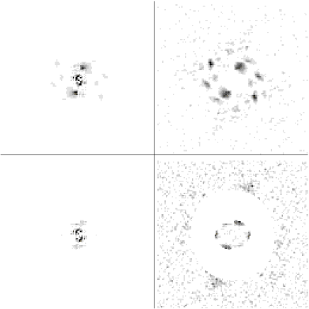
Figure 5: These images show the contribution of each pixel to the symmetry $\chi^{2}$ for visit 11, using the best-fit optical galaxy positions. The top-left image shows the per-pixel $\chi^{2}$ contributions when no masking is used and no PSF error is used. The image on the top-right shows the contributions when no masking is applied and a 7% PSF error is used. The bottom-left image shows the contributions when spiral arms are masked, with no PSF error. The bottom-right image shows the $\chi^{2}$ contributions when the prominent spiral arms are masked and a 7% PSF error is used. All images are 128 pixels (3.2″) in both width and height.

Deriving errors on position from the individual visits is difficult because the symmetry $\chi^{2}$ increases very rapidly away from the minimum. An error measure derived from the shape of the minimum for a single visit implies a spuriously high accuracy for the galaxy position. It is likely that the number of degrees of freedom in the fit is over-estimated and that many pixels do not contribute any useful information to the fit statistic, since the drizzling process introduces correlations between neighbouring drizzled pixels. However, the scatter between positions derived from different visits is large. We therefore estimate errors on the galaxy position by taking ellipses that enclose 68% and 95% of the measurements from all visits to define our $1\,\sigma$ and $2\,\sigma$ confidence levels. Figure 6 shows the 95% confidence ellipses on the galaxy position for both sets of fits, as well as the position derived from LensClean applied to VLA data by Wucknitz et al. (2004).

The positions obtained from the symmetry fits were combined with the extra constraints available from the VLBI substructure described in Patnaik et al. (1995) and Kemball et al. (2001), which were used to constrain mass models by Wucknitz (2004). The optical galaxy position was combined with the models of Wucknitz (2004) by adding $\chi^{2}$ values for the galaxy position to the $\chi^{2}$ values from the lens models. However, the $\chi^{2}$ values taken from the symmetry fitting grid have too many degrees of freedom, and so we assume that the optical position minimum is parabolic and form a new $\chi^{2}$ statistic based on our 68% and 95% confidence ellipses. We define the new $\chi^{2}$ statistic to have a value of 2.31 on our 68% confidence ellipse, and a value of 5.99 on the 95% ellipse, and sum this statistic with that from the lens modelling. We emphasize that the scatter between visits dominates the random error budget for our measurement of $H_{0}$.

Combining the VLBI and optical constraints shows that the best-fit galaxy position and the optical galaxy position are not coincident, as shown in Table 3. The galaxy position shifts by up to 13 mas between the optical fit and the optical+VLBI fit. The shapes of the confidence regions are also altered. However, the value of $H_{0}$ is not very sensitive to this mainly northerly shift.

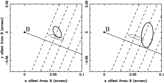
Figure 6: The optical galaxy position compared to that determined by Wucknitz et al. (2004) using LensClean. The error ellipses are 95% confidence regions. The left-hand plot is for the case with no masking. The right-hand plot represents the case with masking of spiral arms. The position of B is marked, as is a line pointing towards the A component. The dotted lines are contours of $H_{0}$ in the strictly isothermal case, and correspond (from right to left) to $H_{0}$ = (90,80,70,60,50) km s^-1 Mpc^-1. The positions determined from optical data are shown as bold ellipses.

Data used	Masking	Mass profile	Position (mas)		$H_{0}$	$H_{0}$	$\beta$	Ellipticity
			$\Delta\alpha$	$\Delta\delta$	(isothermal)	(variable $\beta$)		(of potential)
Optical	None	-	$+$57	$+$0	79$\pm$7	68$\pm$6	1.13${}^{+0.07}_{-0.09}$	0.08$\pm$0.03
Optical	Spiral	-	$+$75	$-$5	66$\pm$9	56${}^{+12}_{-15}$	1.16$\pm$0.19	0.05$\pm$0.04
VLBI+Optical	None	Isothermal	$+$60	$-$13	74$\pm$5	-	-	0.05$\pm$0.02
VLBI+Optical	Spiral	Isothermal	$+$74	$-$19	64$\pm$7	-	-	0.03$\pm$0.02
VLBI+Optical	None	Variable	$+$60	$-$12	-	70$\pm$5	1.05$\pm$0.03	0.04$\pm$0.02
VLBI+Optical	Spiral	Variable	$+$74	$-$18	-	61$\pm$7	1.05$\pm$0.04	0.04$\pm$0.02

Table 3: Lens galaxy positions and the corresponding values of $H_{0}$ and the mass profile slope $\beta$. The optical positions are derived from the ACS images only. The “VLBI+Optical” positions incorporate constraints from the LensClean-based lens modelling of Wucknitz et al. (2004). The “Mass profile” column indicates what mass profile was assumed when combining the VLBI and optical constraints. $H_{0}$ values are given in km s^-1 Mpc^-1. Position offsets are referenced to image B, and RA offsets are given taking west as positive. All errors are quoted at 95% confidence.

6 Extraction of $\mn@boldsymbol{H_{0}}$

The general relation between the time delay $\Delta t_{i,j}$ between the $i^{th}$ and $j^{th}$ images, the Hubble constant $H_{0}$ and the lens model, parametrised by the potential $\psi$, is given by

$$c\,\Delta t_{i,j}=\frac{1+z_{\mathrm{d}}}{H_{0}}\frac{d_{\mathrm{d}}\,d_{\mathrm{s}}}{d_{\mathrm{ds}}}{\left(\phi_{i}-\phi_{j}\right)}\quad\text{,}$$ (4)

where $z_{\mathrm{d}}$ is the redshift of the lens, $d_{\mathrm{d}}$ and $d_{\mathrm{s}}$ are the angular size distances to the lens and source, respectively, $d_{\mathrm{ds}}$ is the angular size distance to the source measured from the lens, and $\phi_{i}$ is the scaled time delay at the position of the $i^{th}$ image ($\mn@boldsymbol{\theta}_{i}$),

$$\phi_{i}=\frac{1}{2}|\nabla\psi(\mn@boldsymbol{\theta}_{i})|^{2}-\psi(\mn@boldsymbol{\theta}_{i})\quad\text{.}$$ (5)

The angular size distances are normalized in these equations, since they do not include factors of $H_{0}$. For general isothermal models without external shear the relation becomes particularly simple and can be written as a function of the image positions alone, without explicitly using any lens model parameters (Witt et al. 2000):

$$\phi_{i}=\frac{1}{2}|\mn@boldsymbol{\theta}_{i}-\mn@boldsymbol{\theta}_{0}|^{2}$$ (6)

Here $\mn@boldsymbol{\mn@boldsymbol{\theta}}_{0}$ is the position of the centre of the lens. External shear $\gamma$ changes $\phi_{i}$ by a factor between $1\pm\gamma$ depending on the relative direction, typically resulting in similar factors for the value deduced for $H_{0}$. A general analysis for power-law models with external shear can be found in Wucknitz (2002).

Using the recipe described in previous sections our lens position translates to a Hubble constant of H${}_{0}=79\pm 7$ km s^-1 Mpc^-1in the shearless isothermal case without masking, and to $66\pm 9$ with masking.

Estimates of external shear and convergence from nearby field galaxies and large scale structure are of the order 2 per cent (Lehár et al. 2000) and would affect the result only to the same relative amount, sufficiently below our current error estimate to allow us to neglect these effects.

The value of the Hubble constant we derive depends on the slope of the mass distribution of the lensing galaxy. In Figure 7 we show the permitted values of the Hubble constant for different models – isothermal and with a variable $\beta$ in an elliptical potential model – plotted against measured galaxy position. The elliptical power-law potential is parametrised as follows:

$$\psi(\mn@boldsymbol{\theta})=\frac{\theta_{\mathrm{E}}^{2-\beta}}{\beta}\,r_{\epsilon}^{\beta}(\mn@boldsymbol{\theta})\quad\text{,}$$ (7)

$$r_{\epsilon}^{2}=\frac{\theta_{x}^{2}}{(1+\epsilon)^{2}}+\frac{\theta_{y}^{2}}{(1-\epsilon)^{2}}\quad\text{,}$$ (8)

$$\mn@boldsymbol{\theta}=(\theta_{x},\theta_{y})\quad\text{,}$$ (9)

where $\theta_{E}$ is the Einstein radius of the model, $\beta$ is the power-law index of the potential’s profile and $\epsilon$ is the ellipticity of the potential. For details of our modelling procedure the reader is referred to Wucknitz et al. (2004). It is evident that the preferred value of the Hubble constant is somewhat reduced compared to what is obtained by forcing the mass distribution to be isothermal. We also show contours of the radial power law $\beta$ plotted against galaxy position. The optical lens position gives $\beta=$1.13${}^{+0.07}_{-0.09}$ ($2\,\sigma$).

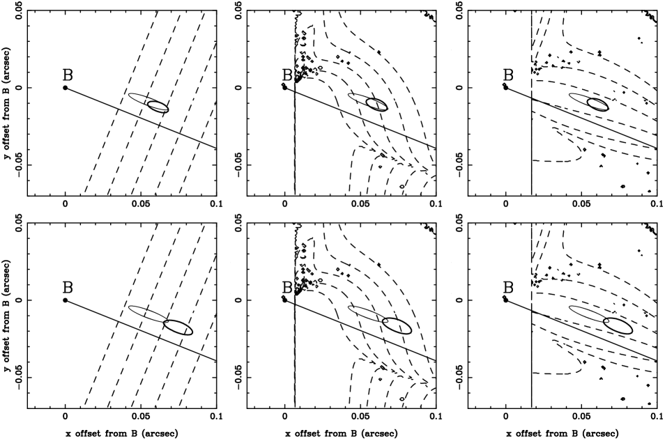
Figure 7: The 95% confidence regions for the cases of no masking (top row) and masked spiral arms (bottom row). The plots in the left-hand column show the galaxy position confidence regions and contours of $H_{0}$ calculated for isothermal models. The plots of the central column show the confidence regions superimposed over contours of $H_{0}$ calculated whilst allowing the logarithmic mass slope $\beta$ to vary. This reduces $H_{0}$ slightly compared to the fixed $\beta=1$ (isothermal) case. The plots in the right-hand column show the same confidence regions superimposed over contours of $\beta$. The confidence regions take both our optical position and the VLBI constraints used by Wucknitz et al. (2004) into account. The 95% confidence error ellipse of Wucknitz et al. is also shown. Contours of $H_{0}$ are again at (90,80,70,60,50)km s^-1 Mpc^-1reading from left to right across an image, and contours of $\beta$ are (0.8,0.9,1.0,1.1,1.2,1.3) reading from bottom to top. The optical+VLBI error ellipses are shown in bold relative to the LensClean ellipse of Wucknitz et al.

As discussed before, B0218+357 has the advantage of clear substructure in the two images which can be mapped with VLBI. The VLBI data can be used independently to derive the slope of the mass profile of the lens (Wucknitz et al., 2004). Biggs et al. (2003) and Wucknitz et al. find a value of $\beta$=1.04$\pm$0.02. Combining the VLBI constraints with the optical lens position gives a value of $\beta$=1.05$\pm$0.03 (95% confidence). We therefore adopt this value for the mass profile’s logarithmic slope and obtain a Hubble constant of 70$\pm$5 km s^-1 Mpc^-1(95% confidence) for the case with no masking and 61$\pm$7 km s^-1 Mpc^-1(95% confidence) when the spiral arms are masked. The ellipticity of the potential is small (about 0.04) in each case, but the ellipticity of the mass distribution will be about three times this, 0.12. The lens galaxy could be more inclined than it appears, or there could be a bar or similar feature present.

7 Conclusions

We have analysed the deepest optical image yet taken of B0218+357 to measure the position of the lens galaxy. We find that simple subtraction of a parametric galaxy model and two point sources is insufficient to constrain the galaxy position, and we confirm earlier suggestions that the image separation in the optical is lower than that in the radio, most probably due to significant extinction around image A. Taking advantage of the symmetric appearance of the lens, we have defined the centre as that point about which the residuals (after subtraction of A and B) are most symmetric. To account for artifacts in our empirical PSF model we have introduced an extra noise term. We have also masked off the most prominent spiral arms to test the effect on $H_{0}$. We find that the lens galaxy position is 57$\pm$4 mas west and 0$\pm$6 mas south of image B when no masking is applied. Combined with the results of Wucknitz et al. (2004) this leads to a value for $H_{0}$ of 70$\pm$5 km s^-1 Mpc^-1(95% confidence). When the most obvious spiral arms are masked out, we find an optical galaxy position of 75$\pm$6 mas west and $-$5$\pm$13 mas south from image B. This results in a value for $H_{0}$ of 61$\pm$7 km s^-1 Mpc^-1(95% confidence) when combined with VLBI constraints.

Further work on this lens will involve increased use of LensClean to further limit the power law exponent $\beta$ using VLBI constraints. Observations have also been made using the VLA with the Pie Town VLBA antenna, which together with VLBI will further improve the lens model for this system.

References

Barkana R., 1997, ApJ, 489, 21

Barkana R., Lehár J., Falco E.E., Grogin N.A., Keeton C.R., Shapiro I.I., 1999, ApJ, 520, 479

Bernstein G., Fischer P., 1999, AJ, 118, 14

Biggs A.D., Browne I.W.A., Helbig P., Koopmans L.V.E., Wilkinson P.N., Perley R.A., 1999, MNRAS, 304, 349

Biggs A.D., Xanthopoulos E., Browne I.W.A., Koopmans L.V.E., Fassnacht C.D., 2000, MNRAS, 318, 73

Biggs A.D., Browne I.W.A., Muxlow T.W.B., Wilkinson P.N., 2001, MNRAS, 322, 821

Biggs A.D., Wucknitz O., Porcas R.W., Browne I.W.A., Jackson N.J., Mao S., Wilkinson P.N., 2003, MNRAS, 338, 599

Browne I.W.A., Patnaik A.R., Walsh D., Wilkinson P.N., 1993, MNRAS, 263, L32

Burud I., Hjorth J., Jaunsen A.O., Andersen M.I., Korhonen H., Clasen J.W., Pelt J., Pijpers F.P., Magain P., Ostensen R., 2000, ApJ, 544, 117

Burud I., Hjorth J., Courbin F., Cohen J.G., Magain P., Jaunsen A.O., Kaas A.A., Faure C., Letawe G., 2002a, A&A, 391, 481

Burud I., et al., 2002b, A&A, 383, 71

Carilli C.L., Rupen M.P., Yanny B., 1993, ApJL, 412, L59

Clampin M., et al., 2000, SPIE, 4013, 344

Cohen, A.S., Hewitt, J.N., Moore, C.B., Haarsma, D.B., 2000, ApJ, 545, 578

Cohen J.G., Lawrence C.R., Blandford R.D., 2003, ApJ, 583, 67

Cohn J.D., Kochanek C.S., McLeod B.A., Keeton C.R., 2001, ApJ, 554, 1216

Combes F., Wiklind T., 1997, ApJ, 486, L79

Ellithorpe J.D., Kochanek C.S., Hewitt J.N., 1996, ApJ, 464, 556

Falco E.E., Gorenstein M.V., Shapiro I.I., 1985, ApJL, 289, L1

Fassnacht C.D., Pearson T.J., Readhead A.C.S., Browne I.W.A., Koopmans L.V.E., Myers S.T., Wilkinson P.N., 1999, ApJ, 527, 498

Fassnacht C.D., Xanthopoulos E., Koopmans L.V.E., Rusin D., 2002, ApJ, 581, 823

Freedman W.L., Madore B.F., Gibson B.K., Ferrarese L., Kelson D.D., Sakai S., Mould J.R., Kennicutt R.C., Jr., Ford H.C., Graham J.A., et al., 2001, ApJ, 553, 47

Fruchter A.S., Hook R.N., 2002, PASP, 114, 144

Gorenstein M.V., Shapiro I.I., Falco E.E., 1988, ApJ, 327, 693

Grundahl F., Hjorth J., 1995, MNRAS, 275, L67

Hack W.J., 2002, in Bohlender D., Durand D., Handley T.H., eds, ASP Conf. Ser. Vol. 281, Astronomical Data Analysis Software and Systems XI. Astron. Soc. Pac., San Francisco, p.197.

Hjorth J., 1997, Helbig P., Jackson N., eds, Proc. Golden Lenses, Hubble’s Constant and Galaxies at High Redshift Workshop. Jodrell Bank Observatory, Cheshire.

Hjorth J., et al., 2002, ApJ, 572, L11

Jackson N., Xanthopoulos E., Browne I.W.A., 2000, MNRAS, 311, 389

Keeton C.R., et al., 2000, ApJ, 542, 74

Kemball A.J., Patnaik A.R., Porcas R.W., 2001, ApJ, 562, 649

Kochanek C.S., Keeton C.R., McLeod B.A., 2001, ApJ, 547, 50

Kochanek C.S., Narayan R., 1992, ApJ, 401, 461

Kochanek C.S., 2002, ApJ, 578, 25

Kochanek C.S., 2003, ApJ, 583, 49

Kochanek C.S., Schechter P., 2004, in “Measuring and Modelling the Universe”, Carnegie Obs. Centennial Symposium, CUP, ed. W. Freedman, p. 117

Koekemoer A.M., Fruchter A.S., Hook R.N., Hack W., 2002, in Arriba S., ed., The 2002 HST Calibration Workshop : Hubble after the Installation of the ACS and the NICMOS Cooling System. Space Telescope Science Institute, Baltimore, MD, p. 339

Koopmans L.V.E., de Bruyn A.G., Xanthopoulos E., Fassnacht C.D., 2000, A&A, 356, 391

Koopmans L.V.E., Fassnacht C.D., 1999, ApJ, 527, 513

Koopmans L.V.E., Treu T., 2003, ApJ, 583, 606

Krist J., 1995, in Shaw R.A., Payne H.E., Hayes J.J.E., eds, ASP Conf. Ser. Vol. 77, Astronomical Data Analysis Software and Systems IV. Astron. Soc. Pac., San Francisco, p. 349

Kundic T., Hogg D.W., Blandford R.D., Cohen J.G., Lubin L.M., Larkin J.E., 1997, AJ, 114, 2276

Landolt A.U., 1992, AJ, 104, 340

Lehár J., Falco E.E., Kochanek C.S., McLeod B.A., Muñoz J.A., Impey C., Rix H., Keeton C.R., Peng C.Y., 2000, ApJ, 536, 584

Lovell J.E.J., Jauncey D.L., Reynolds J.E., Wieringa M.H., King E.A., Tzioumis A.K., McCulloch P.M., Edwards P.G., 1998, ApJ, 508, L51

Mack J., et al., 2003, ACS Data Handbook, Version 2.0 (Baltimore:STScI)

McLure R.J., Kukula M.J., Dunlop J.S., Baum S.A., O’Dea C.P., Hughes D.H., 1999, MNRAS, 308, 377

Menten K.M., Reid M.J., 1996, ApJL, 465, L99

Merline W., Howell S.B., 1995, Expt. Astron., 6, 163

Mould, J.R., et al., 2000, ApJ, 529, 786

Muñoz J.A., Kochanek C.S., Keeton C.R., 2001, ApJ, 558, 657

Mutchler M., Cox C., 2001, Instrument Science Report ACS 2001-07 (Baltimore: STScI)

Ofek E.O., Maoz D., 2003, ApJ, 594, 101

Oscoz A., Alcalde D., SerraRicart M., Mediavilla E., Abajas C., Barrena R., Licandro J., Motta V., Muñoz J.A., 2001, ApJ, 552, 81

Patnaik A.R., Browne I.W.A., Wilkinson P.N., Wrobel J.M., 1992, MNRAS, 254, 655

Patnaik A.R., Browne I.W.A., King L.J., Muxlow T.W.B., Walsh D., Wilkinson P.N., 1993, MNRAS, 261, 435

Patnaik A.R., Porcas R.W., Browne I.W.A., 1995, MNRAS, 274, L5

Patnaik A.R., Narasimha D., 2001, MNRAS, 326, 1403

Pavlovsky C., et al., 2002, ACS Instrument Handbook, Version 3.0 (Baltimore: STScI).

Refsdal S., 1964, MNRAS, 128, 307

Rusin D., Ma C., 2001, ApJL, 549, L33

Saha P., Williams L.L.R., 2001, AJ, 122, 585

Schechter P.L., 2001, in Brainerd T.G., Kochanek C.S., eds, ASP Conf. Ser. Vol. 237, Gravitational Lensing: Recent Progress and Future Goals. Astron. Soc. Pac., San Francisco, p. 427

Schechter P.L., Bailyn C.D., Barr R., Barvainis R., Becker C.M., Bernstein G.M., Blakeslee J.P., Bus S.J., Dressler A., Falco E.E., et al., 1997, ApJL, 475, L85

Stickel M., Kuehr H., 1993, A&AS, 101, 521

Sykes C.M., et al., 1998, MNRAS, 301, 310

Walsh D., Carswell R.F., Weymann R.J., 1979, Nature, 279, 381

Wiklind T., Combes F., 1995, A&A, 299, 382

Williams R.E., et al., 1996, AJ, 112, 1335

Williams L.L.R., Saha P., 2000, AJ, 119, 439

Witt H.J., Mao S., Keeton C.R., 2000, ApJ, 544, 98

Wucknitz O., 2002, MNRAS, 332, 951

Wucknitz O., 2004, MNRAS, 349, 1

Wucknitz O., Biggs A.D., Browne I.W.A., 2004, MNRAS, 349, 14