Multiwavelength Observation of WIMP Annihilation

Abstract

The annihilation of neutralino dark matter may result in observable signals in different wavelength. In the present paper we will discuss the effect of neutralino annihilation in the halo of our Galaxy and in its center. According to high resolution cold dark matter simulations, large virialized halos are formed through the constant merging of smaller halos appeared at previous times. At each epoch, dark matter halos have then a clumpy component which is made of these merging subhalos. The annihilation of dark matter in these clumps, always present in the halo of our Galaxy, may be responsible for appreciable fluxes of $\gamma$-rays, potentially detectable. We find that, depending on the fundamental parameters of the clump density profile and on the distribution of clumps in the Galactic halo, the contribution to the diffuse $\gamma$-ray background from clumps could be used to obtain constraints on the neutralino properties such as mass and annihilation cross section. On the other hand the annihilation of neutralino dark matter in the galactic center may result in radio signals. At the galactic center, infact, the accretion flow onto the central black hole sustains strong magnetic fields that can induce synchrotron emission, in the radio wavelength, by electrons and positrons generated in neutralino annihilations during advection onto the black hole. We find that the observed emission from the galactic center is consistent with neutralinos following a Navarro Frenk and White density profile at the galactic center while it is inconsistent with the presence of a spike density profile, supposed to be generated by the formation history of the central black hole.

1 Introduction

Most of the matter in the universe has yet to be observed in any frequency band, thus the name, dark matter (DM). The evidence for the predominance of dark over visible matter comes mainly from the gravitational effects of the dark matter component. However, gravitational studies have been unable to shed light on the nature of the dark matter. Big bang nucleosynthesis constrains most of the dark matter to be of non-baryonic origin. This has encouraged the study of plausible new particle candidates for the dark matter.

Weakly interacting massive particles (WIMPs) are natural candidates for the dark matter. Particles with masses around $\sim 100$ GeV that interact only weakly have freeze-out densities in the required range of densities. In addition, particle physics models that invoke supersymmetry generate a number of plausible WIMPs. In the supersymmetric extensions of the standard model, the lightest supersymmetric particle may be stable due to conservation of R-parity enabling their survival to the present. In addition to massive and weakly interacting, dark matter particles are expected to be neutral. A class of neutral lightest supersymmetric particles is represented by a combination of gauginos and higgsinos, named the neutralino often represented by $\chi$.

Given the requirements of neutralino production in the early universe, it is possible to study the phenomenology of such dark matter candidates in detail [1]. In particular, the annihilation of neutralinos has often been considered a potential source of detectable secondaries: high energy particles and electromagnetic radiation. In this sense, dark matter can be visible through the radiation caused by the annihilation secondaries [2, 3, 4, 5, 6, 7, 8, 9, 10, 11, 12, 13, 14, 15, 16]. Since the neutralino is a Majorana particle, it will self-annihilate at a rate proportional to the square of neutralino density. Thus, as was first realized in [2], the highest density dark matter regions are the best candidates for indirect searches. In the present paper we will review the annihilation signal that could come from the clumped halo component of our Galaxy and from its Galactic Center (GC), in these regions infact it is expected a large enhancement in the neutralino density with a consequent amplification of the annihilation signal.

Recent advances in Cold Dark Matter (CDM) simulations have shown that the large scale structure of the Universe can be explained in terms of a hierarchical scenario in which large halos of dark matter are generated by the continuous merging of smaller halos [17, 18, 19]. In this picture a dark halo is the superposition of a smooth component, characterized by a typical scale comparable with the virial radius of the forming structure, and a clumped structure made of thousand of small scale halos. CDM simulations also show that most halos are well described by a density distribution with cusps at the center of each halo. The exact shape of the central cusp is still a matter of debate. Most recent simulations favor profiles with density cusps varying from the Moore et al. profile [18] where $\rho_{DM}(r\to 0)\sim r^{-1.5}$ to a Navarro, Frenk, and White (NFW) profile [20] where $\rho_{DM}(r\to 0)\sim r^{-1}$.

The debate is exacerbated by observations of galaxy rotation curves that seem to provide no evidence of central cusps [21]. However, the survival of cusps in galactic centers is highly dependent on the galaxy’s merger history in particular on the history of formation of galactic center black holes [22]. The central regions of small mass dark matter halos (DM clumps) are less affected by the dynamics of baryonic matter and less likely to have black hole (BH) mergers at their centers. Thus, a cuspy profile may well describe the density of DM clumps.

Another important piece of information is embedded in the spatial distribution and survival history of clumps on their way to the central part of the host galactic halo. Much physics is involved in the description of the structure of a DM clump moving in a larger DM halo, and different recipes are possible. These unknowns have forced us to consider two different scenarios, that for simplicity we call type I and type II scenario.

In the type I scenario, the clump position in the host Galaxy determines its external radius. In the case of NFW and Moore profiles, the location of the core is then determined by assuming a fixed fraction of this external radius. In the type II scenario, a recipe is taken from the literature for the so-called concentration parameter, defined as the ratio of the core and virial radii of a clump. The recipe allows one to determine the properties of a clump for a given mass. We show that in this scenario the clumps are gradually destroyed on their way to the center of the Galaxy, so that an inner part, depleted of its clumpy structure is formed. This seems compatible with numerical simulations [23]. The effects of these two scenarios on the $\gamma$-ray emission from the annihilation of CDM particles are dramatic: in the type I scenario, the highly concentrated clumps that are implied produce strong $\gamma$-ray emission while in the type II scenario the low concentration clumps imply $\gamma$-ray fluxes several orders of magnitude smaller than in the previous case.

Another important piece of information could come from the annihilation signal at the GC. Infact, apart from the clumped halo component, the GC region may potentially be so dense that all neutralino models would be ruled out [6]. This strong constrain arises in models where the super-massive BH at the galactic center (GC) induces a strong dark matter density peak called the spike. The existence of such a spike is strongly dependent on the formation history of the galactic center BH [22]. If the BH is formed adiabatically, a spike would be present while a history of major mergers would not allow the survival of a spike.

In contrast to the uncertain presence of a central spike in the dark matter distribution, the central BH is known to induce an accretion flow of baryonic matter around its event horizon. The accretion flow carries magnetic fields, possibly amplified to near equipartition values due to the strong compression. The distribution of electrons and positrons (hereafter called electrons) produced by neutralino annihilation at the GC would also be compressed toward the BH radiating through synchrotron and inverse Compton scattering off the photon background.

By considering the injection of electrons, combined with radiative losses and adiabatic compression, we find the equilibrium spatial and spectral electron distribution and derive the expected radiation signal. We find that the synchrotron emission of electrons from neutralino annihilation range from radio and microwave energies up to the optical, in the central more magnetized region of the accretion flow. At low frequencies, synchrotron self-absorption slightly reduces the amount of radiation transmitted outwards. The resulting signal is stronger than the observed emission in the $10$ to $10^{5}$ GHz range for the case of a spiky dark matter profile while for a pure NFW profile the emission is below the observed values.

The paper is structured as follows in the first three paragraphs we will discuss the annihilation signal that could come, in the $\gamma$-ray frequency range, from the clumped halo of the Galaxy, while in the last three paragraphs we will discuss the synchrotron signal that could come, in the radio frequency range, from the GC. We will conclude in paragraph 7.

2 Dark Matter Clumps in the Halo

The contribution to the diffuse $\gamma$-ray background from $\chi\bar{\chi}$ annihilation in the clumpy halo depends on the distribution of clumps in the halo and on the density profile of these clumps. Our purpose here is to investigate the wide variety of possibilities currently allowed by the results of simulations and suggested by some theoretical arguments, concerning the density profiles of dark matter clumps. We consider three cases: singular isothermal spheres (SIS), Moore et al. profiles, and NFW profiles.

The Moore et al. and the NFW profiles are both the result of fits to different high resolution simulations [18]. Although there is ongoing debate over which profile is most accurate, it is presently believed that a realistic descriptions of the dark matter distribution in halos will follow a profile in the range defined by the Moore et al. and the NFW fits [24]. The dark matter density profiles can be written as follows:

$$\rho_{\chi,{\rm SIS}}(r)=\rho_{0}\left({\frac{r}{r_{0}}}\right)^{-2}.$$ (1)

$$\rho_{\chi,{\rm Moore}}(r)=\frac{\rho_{0}}{\left(\frac{r}{r_{f}}\right)^{3/2}\left[1+\left(\frac{r}{r_{f}}\right)^{3/2}\right]}$$ (2)

$$\rho_{\chi,{\rm NFW}}(r)=\frac{\rho_{0}}{\left(\frac{r}{r_{f}}\right)\left(1+\frac{r}{r_{f}}\right)^{2}}~{}.$$ (3)

The SIS and Moore et al. clump density profiles are in the form given in eqs. (1) and (2) down to a minimum radius, $r_{\rm min}$. Inside $r_{\rm min}$, neutralino annihilations are faster than the cusp formation rate, so that $\rho(r\leq r_{\rm min})=\rho(r_{\rm min})$ remains constant. To estimate $r_{\rm min}$, following [2], we set the annihilation timescale equal to the free-fall timescale, so that

$$r_{\rm min,SIS}=r_{0}\left[\frac{\langle\sigma v\rangle_{Ann}\rho_{0}}{\sqrt{GM_{c}}m_{\chi}}r_{0}^{3/2}\right]^{1/2}\qquad r_{\rm min,Moore}=r_{0}\left[\frac{\langle\sigma v\rangle_{Ann}^{2}\rho_{0}^{2}}{GM_{c}m_{\chi}^{2}}r_{f}^{3}\right]^{1/3},$$ (4)

where $\langle\sigma v\rangle_{Ann}$ is the $\chi\bar{\chi}$ annihilation cross-section, $G$ is the Newton constant, $M_{c}$ and $m_{\chi}$ are respectively the clump mass and the neutralino mass.

The fundamental parameters of the clump density profile are the density normalization $\rho_{0}$, the clump radius $r_{0}$ and, in the case of Moore et al. and NFW profiles, the clump fiducial radius $r_{f}$. In order to fix these fundamental parameters we have considered two different scenarios (type I and II).

We have modeled the smooth galactic halo density with a NFW density profile [Eq. (3)], with $r_{f}=27$ kpc and $\rho_{0}$ determined from the condition that the dark matter density at the Sun’s position is $\rho_{DM}(d_{\odot})=6.5\times 10^{-25}{\rm g/cm}^{3}$.

In the type I scenario, the radius of a clump with fixed mass is determined by its position in the Galactic halo. More specifically, the radius of the clump is located at the radius where the clump density equals the density of the Galactic (smooth) dark matter halo at the clump position (namely $\rho_{0}$). The physical motivation for such a choice is to account for the tidal stripping of the external layers of the clump while the clump is moving in the potential of the host halo. For the NFW and Moore profiles, the fiducial radius $r_{f}$ has been taken as a fixed fraction of $r_{0}$: $r_{f}=0.1r_{0}$.

In the type II scenario the external radius of the clumps is taken to be their virial radius, defined in the usual way: $r_{0}=r_{vir}=\left[\frac{3M_{c}}{4\pi\rho_{200}}\right]^{1/3}$, where $\rho_{200}$ is $200$ times the critical density of the Universe $\rho_{c}=1.88\times 10^{-29}h^{2}$ g/$cm^{3}$ (we have assumed $h=0.7$ everywhere). In this scenario, following [12], we have introduced the concentration parameter defined as $\xi=\frac{r_{0}}{r_{-2}}$, where $r_{-2}$ is the radius at which the effective logarithmic slope of the profile is $-2$, set by the equation $\frac{1}{\rho_{0}}\frac{d}{dr}r^{2}\rho(r)=0$. The mass dependence of the concentration parameter used in our calculations is taken from [25].

The definite trend is that smaller clumps have larger concentration parameter, reflecting the fact that they are formed at earlier epochs, when the Universe was denser. In general, the concentration parameter has also a dependence on the redshift at which the parameter is measured. We are not interested here in such dependence, since we only consider what happens at the present time (zero redshift). The normalization constant in the clump density profile $\rho_{0}$ is fixed by the total clump mass $M_{c}$.

In the case of the NFW density profile $r_{f}=r_{-2}$, while in the case of the Moore et al. density profile $r_{f}=r_{-2}/0.63$ [12]. In terms of concentration parameters $\xi_{NFW}=0.63\xi_{Moore}~{}$. Using the concentration parameter as in [25] for NFW clumps, we can estimate the stripping distance, which we define as the typical distance from the galactic center where the density of a clump of fixed mass and the density in the smooth DM profile are equal at the fiducial radius $r_{f}$ of the clump. In other words, at the stripping distance the layers of the clump outside the fiducial radius will have been stripped off. From this estimate it is easy to see that most clumps in the inner parts of a host galaxy are stripped off of most of their material, so that this region has no clumpy structure. Another way of seeing this phenomenon is that the clumps that are able to reach the central part of the Galaxy are effectively merged to give the observed smooth dark matter profile.

The exception to this conclusion may be represented by low mass clumps, which are more concentrated (denser cores) and may then penetrate deeper. Numerical simulations show the disappearance of large clumps in the centers of galaxy size halos, but they cannot resolve the smaller denser clumps that may eventually make their way into the core of the galaxy. For simplicity, in our calculations we assume that the inner 10 kpc of the Galaxy have no clumps at all.

Figure 1: Flux of $\gamma$-rays in units of (GeV cm² s sr)^-1 arriving on Earth averaged in all directions for $m_{\chi}=$ 100 GeV, $\langle\sigma v\rangle_{Ann}=3\times 10^{-27}$ cm³/s and $M_{c,min}=10^{5}$ $M_{\odot}$. SIS density profile (dotted line), Moore et al. density profile (dashed line) and NFW density profile (continuous line). Also shown is the EGRET data on extragalactic diffuse $\gamma$-ray background (left panel: first scenario; right panel: second scenario).

3 Gamma-ray emission in Neutralino Annihilation

In order to determine the $\gamma$-ray emission from the DM clumps, as already pointed out in the previous section, the distribution of clumps in the Galaxy is needed. The probability distribution function of clumps with a given mass and at a given position can be fitted from numerical simulations. In the present paper we follow [26] adopting a spatial (as a function of the distance $d$ from the galactic center) and mass distribution of the clumps reflecting the following expression:

$$N_{c}(d,M_{c})=N_{c,0}\left(\frac{M_{c}}{M_{H}}\right)^{-\alpha}\left[1+\left(\frac{d}{d_{sc}}\right)^{2}\right]^{-3/2},$$ (5)

where $N_{c,0}$ is a normalization constant and $d_{sc}$ is the scale radius of the clump distribution. Simulations find $\alpha\simeq 1.9$ and a halo like that of our Galaxy, with $M_{H}\simeq 2\times 10^{12}~{}M_{\odot}$, contains about $500$ clumps with mass larger than $10^{8}~{}M_{\odot}$ [17]. The $\gamma$-ray flux per unit solid angle and per unit energy along a fixed line of sight in the $(\theta,\phi)$ direction can be computed as

$$\Phi_{\gamma}(E_{\gamma},\theta,\phi)=\frac{1}{4\pi}\int_{0}^{s_{max}}ds\int_{M_{min}}^{\zeta M_{H}}N_{c}(d(s),M)N_{\gamma}~{}dM$$ (6)

where $d(s)=\sqrt{s^{2}-2sd_{\odot}cos\theta+d_{\odot}^{2}}$ is the distance of a generic point on the line of sight from the galactic center (with $\theta$ the angle between the direction $s$ and the axis Sun-galactic center), $M$ is the clump mass, $\zeta M_{H}$ is the maximum allowed mass for DM clumps in the Halo (we have used $\zeta=0.01$) and $N_{\gamma}$ is the total number of photons emitted per unit time and energy by a DM clump of mass $M$. This quantity, depending on the scenario chosen for the clump density profile, may depend or not on the distance $d(s)$ of the considered point from the galactic center. In the first scenario, where the normalization of the clump density is related to the smooth Halo density, one has $N_{\gamma}=N_{\gamma}(M,d,E_{\gamma})$, while in the second scenario $N_{\gamma}=N_{\gamma}(M,E_{\gamma})$. One should remember that Eq. (6) is an average over all possible realizations of a halo with its clumpy structure. Fluctuations around this value may be present due to the accidental proximity of few clumps in the specific realization that we happen to experience in our Galaxy.

We assume that neutralinos mainly annihilate into quark-antiquark pairs, which seems confirmed by more detailed calculations carried out in specific supersymmetric scenarios [12]. Actually, it is easy to see that even when neutralinos annihilate into pairs of $W^{+}W^{-}$ or $Z^{0}Z^{0}$, the end result of the decay chain is dominated by quarks and antiquarks, hadronizing mainly into pions (roughly 1/3 neutral pions and 2/3 charged pions) and their spectral shape is identical to that of direct quark-antiquark production. In fact, each $W$ or $Z$ boson would have a Lorentz factor $\sim m_{\chi}/M_{Z,W}$ (if the neutralino mass is large enough to allow the production of a $W$ or $Z$ pair). In the rest frame of the boson, the maximum energy of the particles generated in the decay is $M_{Z,W}$, so that in the laboratory frame the spectrum has a cutoff at $m_{\chi}$, as in the case of direct quark production in the neutralino annihilation. The spectrum is also left unchanged.

The number of photons produced with energy $E_{\gamma}$ in a single $\chi\bar{\chi}$ annihilation can be written as follows:

$$\frac{dN_{\gamma}}{dE_{\gamma}}=\int_{E_{\pi,min}}^{E_{\pi,max}}dE_{\pi}P(E_{\pi},E_{\gamma})\frac{dN_{\pi}}{dE_{\pi}}$$ (7)

where $P(E_{\pi},E_{\gamma})=2(E_{\pi}^{2}-m_{\pi}^{2})^{-1/2}$ is the probability per unit energy to produce a $\gamma$-ray with energy $E_{\gamma}$ out of a pion with energy $E_{\pi}$. For the pion fragmentation function we assume the functional form introduced by Hill [27]:

$$\frac{dN_{\pi}}{dE_{\pi}}=\frac{1}{m_{\chi}}\frac{15}{16}x^{-3/2}(1-x)^{2}\,$$ (8)

with $x=E_{\pi}/m_{\chi}$, $E_{\pi,\rm max}=m_{\chi}$ and $E_{\pi,\rm min}=E_{\gamma}+m_{\pi}^{2}/4E_{\gamma}$. Finally,

$$\frac{dN_{\gamma}}{dE_{\gamma}}=\frac{5}{4m_{\chi}}\int_{x_{\rm m}}^{1}dx\frac{(1-x)^{2}}{x^{3/2}(x^{2}-\eta^{2})^{1/2}}~{},$$ (9)

where $\eta=m_{\pi}/m_{\chi}$, and $x_{\rm m}=E_{\gamma}/m_{\chi}+m_{\chi}\eta^{2}/4E_{\gamma}$.

The neutralino annihilation rate per unit volume is, $\Gamma_{\chi\bar{\chi}}(r,M,E_{\gamma})=\rho_{\chi}^{2}(r)\langle\sigma v\rangle_{Ann}/m_{\chi}^{2}$, therefore the $\gamma$-ray emissivity $j_{\gamma}(r,M,E_{\gamma})$ associated to the single clump of mass $M$ is obtained by multiplying Eq. (9) by $\Gamma_{\chi\bar{\chi}}$. The number of $\gamma$-rays produced per unit time and per unit energy in a single DM clump of mass $M$ is then

$$N_{\gamma}(M,E_{\gamma})=\int_{0}^{r_{0}}dr4\pi r^{2}j_{\gamma}(r,M,E_{\gamma})~{}.$$ (10)

4 Gamma Ray Emission from Clumps

In this section we present the results of our calculations of the $\gamma$-ray emission from dark matter annihilation in the halo of our Galaxy, including both the smooth and clumped components introduced above. We detail the description of these results for the two scenarios (type I and II) of spatial distribution of the clumped component. We expect the type II scenario to result in a quite weaker signal than that obtained in the type I scenario, because the recipe for the type I clumps implies much stronger concentration. In the type II scenario the $\gamma$-ray signal from clumps overcomes the $\gamma$-ray flux from the smooth dark matter distribution only in the direction of the galactic anticenter and only for SIS and Moore profiles for the dark matter distribution inside the clumps.

On the other hand, in the type II scenario the contribution of the clumped component to the diffuse $\gamma$-ray flux from the galactic halo is several orders of magnitude above the smooth halo component, for any of the three density profiles considered above. This impressive difference in the predictions is symptomatic of a large uncertainty in the physics involved in the formation and survival of dark matter substructures.

In Fig. 1 we plot the flux of $\gamma$-rays in units of (GeV cm² s sr)^-1 arriving on Earth averaged in all directions for $m_{\chi}=$100 GeV and with $\langle\sigma v\rangle_{Ann}=3\times 10^{-27}$ cm³/s. The curves refer to the $\gamma$-ray flux due to the full dark matter profile, made of the smooth and clumped components. For the type II scenario, the $\gamma$-ray flux contributed by the clumped component is comparable to the contribution of the smooth dark matter profile, while for the type I scenario, the clumpy component is overwhelmingly larger than that due to the smooth component.

The fluxes plotted in Fig. 1 are obtained choosing the minimum clump mass of $M_{c,min}=10^{5}M_{\odot}$, but the dependence of these fluxes on the value of $M_{c,min}$ is only logarithmic. In both figures the dotted, dashed and solid lines correspond to SIS, Moore and NFW clump density profiles respectively.

Also shown are the EGRET data (straight line) on the extragalactic diffuse $\gamma$-ray background which can be fitted from 30 MeV to $\sim$ 30 GeV by [28] ${\frac{dN_{eg}}{d\Omega dE}}=1.36\times 10^{-6}\left(\frac{E}{{\rm GeV}}\right)^{-2.10}{\rm GeV}^{-1}{\rm cm}^{-2}{\rm s}^{-1}{\rm sr}^{-1}$. Depending on the density profile the fluxes have different scalings with the neutralino parameters $m_{\chi}$ and $\langle\sigma v\rangle_{Ann}$:

$$\Phi_{SIS}\propto\langle\sigma v\rangle_{Ann}^{1/2}m_{\chi}^{-5/2}\qquad\Phi_{NFW,Moore}\propto\langle\sigma v\rangle_{Ann}m_{\chi}^{-3}~{},$$ (11)

these scalings are the same for the type I and II scenarios.

It is clear from Fig. 1 that the comparison between our predictions and the observed diffuse background is meaningful only for the type I scenario, with highly concentrated clumps. In the second scenario, the fluxes are too low, with the exception of the case in which the density profile is the SIS one. For the other cases the region of parameters that can be constrained is already ruled out from accelerator experiments $m_{\chi}\geq 50$ GeV [29] and from theoretical arguments $\langle\sigma v\rangle_{Ann}\leq 10^{-26}$cm³/s [30].

Figure 2: Limits on the neutralino parameter space in the first scenario for clump density profile.

The situation is different for the type I scenario. As anticipated above, all the density profiles imply $\gamma$-ray fluxes comparable to or largely in excess of the EGRET observations of the diffuse $\gamma$-ray background. These observations may therefore be used as a tool to extract severe constraints on the neutralino parameter space, which unfortunately are restricted to the type I scenario. Using the scalings given above (cfr. Eq. (11)), we can determine the regions of the parameter space which are ruled out by our calculations.

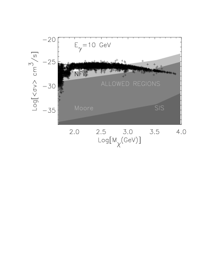
Using EGRET data at 10 GeV, we find that SIS clumps in our halo are ruled out in the region $\langle\sigma v\rangle_{Ann}\geq 2\times 10^{-35}(m_{\chi}/{\rm 100GeV})^{2}{\rm cm}^{3}/{\rm s}$ for $50GeV\leq m_{\chi}\leq 3TeV$, and $\langle\sigma v\rangle_{Ann}\geq 6\times 10^{-40}(m_{\chi}/{\rm 100GeV})^{5}{\rm cm}^{3}/{\rm s}$ cm³/s for $m_{\chi}\geq 3$ TeV.

Moore et al. clumps are also strongly constrained: the 10 GeV EGRET data require that $\langle\sigma v\rangle_{Ann}\leq 2.5\times 10^{-28}(m_{\chi}/{\rm 100GeV})^{3/2}{\rm cm}^{3}/{\rm s}$ for $50GeV\leq m_{\chi}\leq 3TeV$, and $\langle\sigma v\rangle_{Ann}\leq 10^{-30}(m_{\chi}/{\rm 100GeV})^{3}{\rm cm}^{3}/{\rm s}$ for $m_{\chi}\geq 3$ TeV.

If we extrapolate the EGRET measurement of the extragalactic diffuse $\gamma$-ray background to 100 GeV, the bounds get tighter: for $m_{\chi}$ between 50 GeV and 30 TeV, the flux from clumps is below the EGRET data if $\langle\sigma v\rangle_{Ann}\leq 6\times 10^{-29}(m_{\chi}/{\rm 100GeV})^{3/2}$ cm³/s, while for $m_{\chi}\geq 30$ TeV, the region $\langle\sigma v\rangle_{Ann}\leq 10^{-32}(m_{\chi}/{\rm 100GeV})^{3}$ cm³/s is allowed.

The NFW clumps in the type I scenario are the ones that are more weakly constrained. The bounds that can be placed by EGRET at 10 GeV are as follows: if $m_{\chi}$ is between 50 GeV and 3 TeV, the allowed region is defined by $\langle\sigma v\rangle_{Ann}\leq 10^{-26}(m_{\chi}/{\rm 100GeV})^{3/2}$ cm³/s. For $m_{\chi}\geq 3$ TeV, the allowed region is instead $\langle\sigma v\rangle_{Ann}\leq 6\times 10^{-29}(m_{\chi}/{\rm 100GeV})^{3}$ cm³/s. If we extrapolate EGRET data up to 100 GeV, the bounds become as follows: for $m_{\chi}$ between 50 GeV and 30 TeV, one must have $\langle\sigma v\rangle_{Ann}\leq 3\times 10^{-27}(m_{\chi}/{\rm 100GeV})^{3/2}$ cm³/s while for $m_{\chi}\geq 30$ TeV, the allowed region becomes $\langle\sigma v\rangle_{Ann}\leq 5\times 10^{-31}(m_{\chi}/{\rm 100GeV})^{3}$ cm³/s. All these bounds are shown in Fig. 2. The scatter plot reported in Fig. 2 represents all the admitted values of $(m_{\chi},\langle\sigma v\rangle_{Ann})$ allowed by SUSY models [30].

5 Dark Matter and Magnetic Field at the GC

The possibility of detecting neutralino annihilation trough the $\gamma$-ray emission, as discussed in the previous sections, is not the only one. Another appealing possibility is related to the synchrotron emission of electron-positron pairs produced by neutralino annihilation at the GC. In this section we will discuss the major characteristics of the DM density profile at the GC, taking also into account the effects on the GC magnetic field of the advection flow produced by the central BH.

The spatial distribution of dark matter in galactic halos is still a matter of much debate (see, e.g., [24]). Numerical simulations suggest that collisionless dark matter forms cuspy halos while some observations argue for a flat inner density profile [21]. The standard numerical dark matter halo is the NFW profile [20] which is expected to be universal. However, recent simulations have found more cuspy halos [18] as well as shallower profiles [23]. At present, it is not clear if there is a universal dark matter halo profile, but the NFW profile seems to represent well the range of possibilities. Therefore, we assume that the NFW profile describes well the dark matter in our Galaxy and we will use the NFW profile with the parameters introduced in §2.

There is now growing evidence for the presence of a supermassive BH at the GC, with mass $\sim 2\times 10^{6}M_{\odot}$. In fact most galaxies seem to have central black holes with comparable or even larger masses. The presence of a BH can steepen the density profile of dark matter by transforming the cusp at the GC into a spike of dark matter [4]. The density profile of the spike region, where the gravitational potential is dominated by the BH is described by

$$\rho^{\prime}_{sp}(r)=\alpha_{\delta}^{\delta_{sp}-\delta}\left(\frac{M}{\rho_{\odot}R_{\odot}^{3}}\right)^{(3-\delta)(\delta_{sp}-\delta)}\rho_{\odot}g(r)\left(\frac{R_{\odot}}{r}\right)^{\gamma_{sp}}.$$ (12)

Here, $\delta$ is the slope of the density profile of dark matter in the inner region ($\delta=1$ for a NFW profile), and $\delta_{sp}=(9-2\delta)/(4-\delta)$. The coefficients $\alpha_{\delta}$ and $g(r)$ can be calculated numerically as explained in detail in [4]. It is possible to identify a spike radius $R_{sp}$ where the spike density profile given in Eq. (12) matches the NFW dark matter profile. In other words, at $R_{sp}$ the gravitational potential is no longer dominated by the central BH.

Neutralino annihilations affect the density profile in the spike by generating a flattening where the annihilation time becomes smaller than the age of the BH. This effect produces a constant neutralino density given by $\rho_{core}=\frac{m_{\chi}}{\langle\sigma v\rangle_{Ann}t_{BH}}$, where $t_{BH}$ is the BH age. The effect of annihilations on the spike density profile can be written as

$$\rho_{sp}(r)=\frac{\rho^{\prime}_{sp}(r)\rho_{core}}{\rho^{\prime}_{sp}(r)+\rho_{core}},$$ (13)

which accounts for the flattening in the central region.

Several dynamical effects may weaken or destroy the spike in the GC [1, 22], depending on the history of formation of the central BH. If the spike is not formed or gets destroy, the central region should be described by the cuspy profile such as in the NFW case. Here we consider both cases and show that the observed emission is stronger than the predictions for a NFW cusp, while the spike generates signals well above the observations.

In order to determine the synchrotron emission produced by the electrons that come from neutralino annihilations it is necessary to determine the magnetic field present in the GC region. In what follows we will determine the magnetic field strength assuming the equipartition between magnetic field energy and the kinetic pressure due to the accretion flow inside the central BH.

We model the accretion flow of gas onto the BH at the center of our Galaxy following a simple approach described in [31]. More detailed models of the accretion flow around the BH lead to corrections which are negligible when compared to the uncertainties in the dark matter distribution. In the model we adopt, the BH accretes its fuel from a nearby molecular cloud, located at about $0.01$ pc from the BH. The accretion is assumed to be spherically symmetric Bondi accretion with a rate of mass accretion of $\dot{M}=10^{22}\dot{M}_{22}~{}\rm g~{}s^{-1}$. The accretion onto the BH occurs with a velocity around the free-fall velocity, such that

$$v(r)=\sqrt{2GM_{BH}/r}=c\left(\frac{R_{g}}{r}\right)^{1/2}$$ (14)

where $R_{g}=2GM_{BH}/c^{2}=7.4\times 10^{11}(M_{BH}/2.5\times 10^{6}M_{\odot})~{}\rm cm$ is the gravitational radius of the BH and $M_{BH}$ is the BH mass. Therefore,

$$v(r)=1.46\times 10^{8}\left(\frac{M_{BH}}{2.5\times 10^{6}M_{\odot}}\right)^{1/2}\left(\frac{r}{0.01\rm pc}\right)^{-1/2}~{}\rm cm~{}s^{-1}.$$ (15)

Mass conservation then gives the following density profile:

$$\rho(r)=\frac{\dot{M}}{4\pi r^{2}v(r)}=\frac{\dot{M}}{4\pi R_{g}^{2}c}\left(\frac{r}{R_{g}}\right)^{-3/2}\ ,$$ (16)

such that

$$\rho(r)=5.6\times 10^{-21}\dot{M}_{22}\left(\frac{M_{BH}}{2.5\times 10^{6}M_{\odot}}\right)^{-1/2}\left(\frac{r}{0.01\rm pc}\right)^{-3/2}~{}\rm g~{}cm^{-3}\ .$$ (17)

Following [31], we assume that the magnetic field in the accretion flow achieves its equipartition value with the kinetic pressure, namely $\rho v^{2}/2=B(r)^{2}/8\pi$. With this assumption,

$$B_{eq}(r)=\frac{\sqrt{\dot{M}c}}{R_{g}}\left(\frac{r}{R_{g}}\right)^{-5/4}=3.9\times 10^{4}\dot{M}_{22}M_{BH}^{1/4}\left(\frac{r}{0.01\rm pc}\right)^{-5/4}\quad\mu{\rm G}.$$ (18)

It is believed that magnetic fields in the accretion flow will in general reach the equipartition values described in Eq. (18). However, smaller fields may be reached if the equipartition is prevented somehow. In what follows we will always assume the equipartition field in deriving the synchrotron signal from electrons produced by neutralino annihilation.

6 Neutralino Annihilation at the GC

Following our discussion of section §3 we will assume that neutrino annihilation channel is dominated by quark-antiquark production, with a large production of pions described, as already discussed in §3, by the Hill [27] spectrum.

The spectrum of electrons (and positrons) from the $\pi^{\pm}$ decays is calculated by convoluting the spectrum of pions and muons. For relativistic electrons the electron spectrum reads

$$W_{e}(E_{e})=\int_{{\rm max}(E_{e},m_{\mu})}^{m_{\chi}}dE_{\mu}\int_{E_{\pi}^{{\rm min}}}^{E_{\pi}^{{\rm max}}}dE_{\pi}W_{\pi}(E_{\pi})\frac{m_{\pi}^{2}}{m_{\pi}^{2}-m_{\mu}^{2}}\frac{1}{\sqrt{E_{\pi}^{2}-m_{\pi}^{2}}}\frac{dn_{e}(E_{e},E_{\mu},E_{\pi})}{dE_{e}},$$ (19)

where, neglecting the muon polarization, we get

$$\frac{dn_{e}(E_{e},E_{\mu},E_{\pi})}{dE_{e}}=\frac{1}{E_{\mu}\beta}\left\{\begin{array}[]{ll}2\left[\frac{5}{6}-\frac{3}{2}\epsilon^{2}+\frac{2}{3}\epsilon^{3}\right]&{\rm if}~{}~{}~{}\frac{1-\beta}{1+\beta}\leq\epsilon\leq 1\\ \frac{4\epsilon^{2}\beta}{(1-\beta)^{2}}\left[3-\frac{2}{3}\epsilon\left(\frac{3+\beta^{2}}{1-\beta}\right)^{2}\right]&{\rm if}~{}~{}~{}0\leq\epsilon\leq\frac{1-\beta}{1+\beta},\end{array}\right.$$ (20)

with $\epsilon=\frac{2}{1+\beta}\frac{E_{e}}{E_{\mu}}$. Here $\beta$ is the pion speed and $E_{e}$ and $E_{\mu}$ are the total energies of electrons and muons respectively. The two limits of integration $E_{\pi}^{{\rm min}}(E_{\mu})$ and $E_{\pi}^{{\rm max}}(E_{\mu})$ can be derived by inverting the following equations:

$$E_{\mu}\leq\frac{E_{\pi}}{2m_{\pi}^{2}}\left[m_{\pi}^{2}(1+\beta)+m_{\mu}^{2}(1-\beta)\right]$$ (21)

$$E_{\mu}\geq\frac{E_{\pi}}{2m_{\pi}^{2}}\left[m_{\pi}^{2}(1-\beta)+m_{\mu}^{2}(1+\beta)\right]~{}.$$ (22)

Finally, the injection of new electrons, produced in neutralino annihilation, at the distance $r$ from the BH and at energy $E$ can be written as $Q(E,r)=(1/2)(\rho_{DM}(r)/m_{\chi})^{2}W_{e}(E)\langle\sigma v\rangle_{Ann}$, where the density of dark matter has the profile $\rho_{DM}(r)$ discussed in §5 (NFW or spike).

The spectrum of particles at a position $r$ in the accretion flow around the BH is the result of the injection on newly produced electrons at the same position, radiative losses of these electrons and the adiabatic compression that may enhance their momentum while they move inward. Here we neglect spatial diffusion, which occurs on larger time scales.

The transport equation including all these effects can be written as follows:

$$v(r)\frac{\partial f}{\partial r}-\frac{1}{3r^{2}}\frac{\partial}{\partial r}\left[r^{2}v(r)\right]~{}p~{}\frac{\partial f}{\partial p}+\frac{1}{p^{2}}\frac{\partial}{\partial p}\left[p^{2}\dot{p}(r,p)f\right]=Q(r,p),$$ (23)

where $f(r,p)$ is the equilibrium distribution function of electrons injected according with $Q(r,p)$, and losing energy radiatively as described by the function $\dot{p}(r,p)=dp(r,p)/dt$. Here $v(r)=-c(r/R_{g})^{-1/2}$ is the inflow velocity. The equation can be solved analytically if the electrons remain relativistic everywhere in the fluid. The assumption of relativistic electrons can be safely used as discussed in [16]. In Eq. (23), the term

$$\dot{p}_{ad}=-\frac{1}{3}p\nabla v(r)=-\frac{1}{3r^{2}}p\frac{\partial}{\partial r}\left[r^{2}~{}v(r)\right]$$ (24)

describes the rate of change of momentum of a particle at the position $r$ due to adiabatic compression in the accretion flow. The rate of adiabatic momentum enhancement should be compared with the rate of losses due to synchrotron emission:

$$\dot{p}_{syn}(r,p)=\frac{4}{3}\sigma_{T}\frac{B^{2}(r)}{8\pi}\gamma^{2},$$ (25)

where $\sigma_{T}$ is the Thomson cross section and $\gamma$ is the Lorentz factor of the electron. The magnetic field $B_{eq}(r)$ depends on $r$ as described in Eq. (18).

In order to solve the transport equation, Eq. (23), we discuss different loss processes using the equipartition field $B_{eq}$. We first consider synchrotron losses ($\dot{p}_{syn}$), followed by inverse Compton losses ($\dot{p}_{ICS}$) and synchrotron self-compton scattering ($\dot{p}_{SSC}$). The rate of synchrotron losses from Eq. (25) is given by: $\dot{p}_{syn}(r,p)~{}c=1.6\times 10^{-18}\left(\frac{r}{0.01\rm pc}\right)^{-5/2}~{}\gamma^{2}~{}\rm erg~{}s^{-1}$. In the Thomson regime, losses due to Inverse Compton Scattering (ICS) off a photon background with energy density $U_{ph}$ has the following form $\dot{p}_{ICS}(r,p)=\frac{4}{3}\sigma_{T}U_{ph}\gamma^{2}$, ICS dominates synchrotron losses only if $B^{2}>8\pi U_{ph}$. Assuming that $U_{ph}$ is independent of $r$ (i.e. a fixed photon background) ICS becomes important at large radii ($\sim 0.01\rm pc$) and only if $U_{ph}\geq 10^{4}\rm eV~{}cm^{-3}$. Such a strong photon background is unlikely to be present at the GC region. For comparison, the CMB radiation has $U_{CMB}\approx 0.25\rm eV~{}cm^{-3}$ while the optical background has $U_{opt}\approx 1\rm eV~{}cm^{-3}$. If ICS off a fixed background is not dominant at large radii, it becomes even less important as small radii when compared to synchrotron losses. Consequently, we safely neglect the role of ICS off photons of fixed photon backgrounds.

The electrons, radiating in the strong magnetic field near the BH generate a photon background that can become quite intense. The rate of losses due to ICS of electrons off the photons generated through synchrotron emission by the same electrons is $\dot{p}_{SSC}(r,p)=\frac{4}{3}\sigma_{T}U_{ph}^{syn}(r)\gamma^{2}$, where the photon energy density generally depends on the radius $r$. The photon density $U_{ph}^{syn}(r)$ is a nonlinear function of the distribution $f(r,p)$. In other words, the term $\dot{p}$ in Eq. (23) depends in turn on $f(r,p)$ when synchrotron self-Compton scattering is included. If this contribution cannot be neglected, an analytical solution of the transport equation becomes unattainable.

Figure 3: Electron density per unit energy as a function of energy (solid lines) at $r=10^{3}R_{g}$ (upper curve) and $r=10^{4}R_{g}$ (lower curve). Superimposed (dashed curves), we plot the function $n(E,r)$ obtained without the effect of advection. The left panel illustrates the spike case, while the right panel applies to the NFW case.

Given the distribution function $f(r,p)$, one can calculate the synchrotron emissivity $j(\nu,r)$ (energy per unit volume, per unit frequency, per unit time). The photon energy density at the position $r$ is then proportional to the integration over all lines of sight of the emissivity, with the possible synchrotron self-absorption taken into account at each frequency. However, the distribution function $f(r,p)$ is not known a priori, and the problem becomes intrinsically nonlinear. The approach that we follow here is start with neglecting synchrotron self-Compton scattering and check a posteriori whether the assumption is correct in the situation at hand.

An analytic solution of the transport equation can be derived when $\dot{p}(r,p)$ is dominated by synchrotron losses as in Eq. (25). In this case, the equation admits the following analytical solution:

$$f(r,p)=\frac{1}{c}\left(\frac{r}{R_{g}}\right)^{-2}\int_{r}^{R_{acc}}dR_{inj}\left(\frac{p_{inj}}{p}\right)^{4}\left(\frac{R_{inj}}{R_{g}}\right)^{5/2}Q(R_{inj},p_{inj})~{}.$$ (26)

The function $p_{inj}=p_{inj}[p,r,R_{inj}]$ corresponds to the injection momentum of an electron injected at the position $R_{inj}$ that arrives at the position $r$ with momentum $p$. This injection momentum can be obtained by inverting, with respect to $p_{inj}$ the solution of the equation of motion of the electron, in the presence of adiabatic compression and radiative losses:

$$\frac{dp}{dr}=\frac{k_{0}}{c}\left(\frac{r}{R_{g}}\right)^{-2}p^{2}-\frac{1}{2R_{g}}~{}p~{}\left(\frac{r}{R_{g}}\right)^{-1}.$$ (27)

The solution of this equation, with initial condition $p[r=R_{inj},p_{inj},R_{inj}]=p_{inj}$ is

$$p[r,p_{inj},R_{inj}]=p_{inj}\left[\frac{2k_{0}}{3c}\frac{R_{g}^{2}}{r}p_{inj}\left[1-\left(\frac{r}{R_{inj}}\right)^{3/2}\right]+\left(\frac{r}{R_{inj}}\right)^{1/2}\right]^{-1}~{}.$$ (28)

In the absence of synchrotron energy losses, particle momenta only change due to adiabatic compression, and the momentum of a particle changes according with the well known $p=p_{inj}(r/R_{inj})^{-1/2}$, valid for the case of free fall.

The joint effect of the energy gain due to the adiabatic compression and the energy losses due to synchrotron emission generates a new energy scale $p_{m}$ in the system: $p_{m}=\frac{3rc}{2k_{0}R_{g}^{2}}=\frac{3\pi r(mc)^{2}}{\sigma_{T}\dot{M}}$, where $k_{0}=\sigma_{T}B_{0}^{2}/6\pi(mc)^{2}$ ($k_{0}=0$ no synchrotron losses). Introducing $p_{m}$ we can rewrite $p[r,p_{inj},R_{inj}]$ as:

$$p[r,p_{inj},R_{inj}]=p_{inj}\left[\frac{p_{inj}}{p_{m}}\left(1-\left(\frac{r}{R_{inj}}\right)^{3/2}\right)+\left(\frac{r}{R_{inj}}\right)^{1/2}\right]^{-1}\ .$$ (29)

From this expression it is clear that, at any fixed position $r$, adiabatic compression dominates over synchrotron losses if the injection momentum is lower than $p_{m}$. In this case, the electron energy increases while the electron moves inward, until the rate of synchrotron losses become important. The opposite happens when the electrons are injected at momenta larger than $p_{m}$, since synchrotron losses are important from the time of injection. The momentum $p_{m}$ can be interpreted as the momentum where the two competitive effects of adiabatic heating and synchrotron losses balance each other. Thus, particles accumulate at momentum $p_{m}$. This phenomenon depends on the distance from the galactic center: at large distances from the BH the momentum $p_{m}$, which scales linearly with radius, is large and the local rate of injected electrons is low, therefore, the accumulation is small. At small distances the accumulations at $p_{m}$ grows.

We can define the electron equilibrium spectrum $n(E,r)$ which is related to $f(E,r)$ through the relation $n(E,r)dE=4\pi p^{2}f(p,r)dp$. In Fig. 3 we plot $n(E,r)$, in the two cases of an NFW (right panel) and a spike (left panel) density profiles, as a function of the electron energy at two different radii, $r=10^{3}R_{g}$ (upper solid curve) and $r=10^{4}R_{g}$ (lower solid curve); we have fixed $m_{\chi}=100$ GeV and $\langle\sigma v\rangle_{Ann}=10^{-27}$cm³/s. The dashed lines illustrate the solution of the transport equation when adiabatic compression is switched off and only synchrotron losses are included. The accumulation effect described above manifests itself through the appearance of the spiky structure at momentum $p_{m}$. The accumulation is less pronounced at large radii, as expected.

We conclude this section by addressing the issue of the synchrotron self- Compton scattering. As explained above, this effect cannot be accounted for in an analytical approach to the transport equation, since it is intrinsically nonlinear. Instead, we check a posteriori if neglecting SSC was a good assumption. The photon energy density as a function of $r$, $U_{ph}^{syn}(r)$, is easily calculated on the basis of symmetry arguments:

$$U_{ph}^{syn}(r)=\frac{1}{c}\left[\frac{1}{r^{2}}\int_{r_{min}}^{r}dr^{\prime}r^{\prime 2}\int d\nu j(\nu,r^{\prime})+\int_{r}^{\infty}dr^{\prime}\int d\nu j(\nu,r^{\prime})\right]~{},$$ (30)

where $j(\nu,r)$ is the synchrotron emissivity.

This energy density can now be compared with the magnetic energy density at the same location, $B^{2}(r)/8\pi$. The results are plotted in Fig. 4: the solid line represents the photon energy density $U_{ph}^{syn}(r)$, while the magnetic energy density is plotted as a dashed line. The calculations are carried out for a dark matter density profile with the spike at the center and a neutralino mass of 100 GeV. The magnetic energy always dominates over the photon energy, although at large distances from the BH the difference between the two curves reduces to about one order of magnitude. The curves in Fig.4 are obtained without taking into account the synchrotron self-absorption effect, therefore the calculated photon energy density should be considered as an upper limit. Thus, neglecting SSC is a good approximation for the present scenario.

Let us conclude this section addressing the issue of the synchrotron self-absorption (SSA) mechanism. Synchrotron radiation can be reabsorbed by the radiating electrons when the system is sufficiently compact. This phenomenon is particularly effective at low frequencies.

Figure 4: Comparison between the energy density of the synchrotron emitted photons $U_{ph}$ (solid line) and the energy density associated to the magnetic field $B^{2}/8\pi$ (dashed line).

Following the standard procedure [32] we have included the SSA effect in the emission evaluation finding that this effect is efficient only in the case of the spike density profile and only for frequencies $\nu<10^{11}$ Hz [16]. This results holds only in the case in which both synchrotron losses and adiabatic compression are taken into account. On the other hand if only synchrotron losses are considered the SSA effect becomes important even at lower frequencies. The dependence of the SSA on the neutralino parameters scales with $n(E,r)\propto\langle\sigma v\rangle_{Ann}m_{\chi}^{-3/2}$. At fixed $\langle\sigma v\rangle_{Ann}$, the electron density drops with increased $m_{\chi}$, and the SSA effect decreases as well. Finally, in the case of an NFW density profile without a spike, the rate of electrons injection remains such that the effect of SSA can always be neglected at the frequencies of interest.

7 Synchrotron Emission from the GC

In this section, we present our results in terms of the synchrotron luminosity produced by relativistic electrons from neutralino annihilations in the GC. We have considered both cases of a spike density profile and an NFW density profile. Taking into account the effect of SSA, that is efficient only in the spike case as discussed before, we have computed, through the equilibrium spectrum of electrons $n(E,r)$, the synchrotron luminosity $L_{\nu}$ integrated over the all sky (i.e. over all lines of sight).

In Fig. 5, we fix $m_{\chi}=10^{2}$ GeV and $\langle\sigma v\rangle_{Ann}=10^{-27}$ cm³/s and show the luminosity obtained with both the spike (left panel) and NFW (right panel) density profile for two cases: the continuous line shows the case in which advection is taken into account, while the dashed line shows the case in which only the synchrotron energy losses are present. Comparison of the two curves in Fig. 5 shows that the resonant behavior due to the combined effect of advection and synchrotron losses becomes important for frequencies up to $10^{14}$ Hz. In this frequency range, the electron density is much higher when advection is included as compared to the pure synchrotron case. This effect produces an increase in the emitted luminosity of about one order of magnitude. In addition, we can see that SSA decreases the emitted radiation in the frequency range $10^{10}-10^{11}$ Hz. Moreover, the SSA effect becomes relevant only when advection is taken into account and only in the case of the spike density profile.

In order to constrain the shape of the dark matter density profile at the GC or the parameters of the dark matter particle, we compare the calculated luminosities with the observations. The well-studied source at the GC, Sgr A^∗, has been observed in a large range of frequencies, from the radio up to the near-infrared. Experimental data from $10^{9}$ Hz to $10^{14}$ Hz [33] are displayed in Fig. 6. In the same figure we show the two cases of spiky (left panel) and NFW (right panel) density profile, for $m_{\chi}=10^{2}$ GeV (upper curves) and $m_{\chi}=10^{3}$ GeV (lower curves) and $\langle\sigma v\rangle_{Ann}=10^{-27}$ cm³/s. In Fig. 6 we also show the results for the cases in which only synchrotron losses are taken into account (dashed curves). From Fig. 6, it is clear that a spike in the GC induces much stronger emission than the observed flux. Therefore, either there is no spike in the dark matter profile or neutralinos are not the dark matter. This conclusion agrees with previous studies [6] that show how changes to the neutralino parameter do not gap this large discrepancy. The parameter space for neutralinos $m_{\chi},\langle\sigma v\rangle_{Ann}$ has been studied extensively [6]. From accelerator studies $m_{\chi}=10^{2}$ GeV is a lower limit and from cosmological constraints (i.e., dark matter density) $m_{\chi}$ and $\langle\sigma v\rangle_{Ann}$ must lie in the range: $m_{\chi}\in[10^{2}{\rm GeV},10^{3}{\rm GeV}]$ and $\langle\sigma v\rangle_{Ann}\in[10^{-27}{\rm cm}^{3}{\rm/s},10^{-26}{\rm cm}^{3}{\rm/s}]$ [30].

The emitted luminosity scales with the neutralino mass and the annihilation cross section through the electron density $n(E,r)$, following the same relations obtained in Eq. (11). This implies that the luminosity can only be lowered by at most one order of magnitude, by increasing the neutralino mass up to $\sim$ 1 TeV. While it is easy to increase the luminosity by an order of magnitude without violating any bound simply by increasing the cross section of neutralino annihilation, it is hard to decrease it. In fact, as $\langle\sigma v\rangle_{Ann}$ is lowered well below $10^{-27}$ cm³/s, the density of neutralinos becomes smaller than the necessary density to account for cold dark matter.

The large enhancement of the neutralino density due to the spike profile produces a synchrotron luminosity that is difficult to reconcile with observations. Moreover, this conclusion only gets stronger when advection is included. The SSA effect does not affect the discrepancy between a neutralino spike and the observations, since it changes the luminosity only at frequencies in the range $10^{10}\div 10^{11}$ Hz. The situation is completely different for the case of the NFW density profile. In this case, the synchrotron luminosity is always less than the experimental data as can be seen in Fig. 6. NFW is consistent with observations even if $\langle\sigma v\rangle_{Ann}=10^{-26}$ cm³/s is considered.

Figure 5: Emitted luminosty in two cases: 1) advection and synchrotron losses (solid line); 2) only synchrotron losses (dashed line). The computation is performed with $m_{\chi}=10^{2}$ GeV and $\langle\sigma v\rangle_{Ann}=10^{-27}$ cm³/s. The left panel represents the Spike case while right panel the NFW case.

In this paper, we only considered two possibilities for the dark matter density profile: the less concentrated hypothesis (NFW) and the most concentrated one (spike). Other proposed profiles such as the Moore et al. profile should generate a luminosity in between the spike and the NFW cases. In this case, observations are likely to place more stringent limits on the neutralino parameters instead on the density profile itself.

8 Conclusions

In this paper we have discussed two possible avenues that lead to an indirect detection of the annihilation of neutralino CDM. We have discussed the effect of this annihilation in the halo of our galaxy as well as in its center.

The expected emission from the halo annihilation drops into the $\gamma$-ray frequency range and it generates a diffuse $\gamma$-ray background. The Dark matter sub-structures of the galactic halo can be a dominant component of the diffuse $\gamma$-ray background depending on the concentration and location of DM clumps in the inner regions of the galactic halo. In order to bracket the range of possible fluxes we have considered two extreme scenarios, that we named type I and type II. The first corresponds to extremely concentrated clumps present everywhere in the Galaxy halo, while in the second scenario the clumps are much less concentrated and are completely destroyed by tidal effects in the inner 10 kpc of the Galaxy. While the type I scenario allows one to put very strong constraints on the properties of neutralinos and on the density profile inside clumps, the type II scenario generates fluxes of diffuse $\gamma$-rays which are barely detectable, with the exception of the case in which the density profile of the clumps is modeled as a SIS sphere. For the type I scenario, most of the parameter space of neutralino dark matter is ruled out if the density profile of dark matter clumps is in the form of a SIS sphere or a Moore profile. Weaker bounds can be imposed on the neutralino parameter space in the case of NFW density profile.

Figure 6: Luminosity, compared with experimental data from Sgr A^∗, in the case of the spiky density profile (left panel) and NFW density profile (right panel). Dashed curves represent the luminosity obtained neglecting the effect of advection. The computation is performed with $m_{\chi}=10^{2}$ GeV (upper curves) and $m_{\chi}=10^{3}$ GeV (lower curves). The annihilation cross section is $\langle\sigma v\rangle_{Ann}=10^{-27}$ cm³/s.

The second possibility that we have considered here is related to the electron-positron emission in the GC magnetic field. Electron-positron pairs are expected to be copiously produced in neutralino annihilation, from the comparative study of their synchrotron emission at the GC with the experimental data, already available in the radio and near IR frequency range, we have obtained severe limits on the neutralino density profile at the GC. Using our results we can reaffirm that a spike density profile is ruled out by these radio and near IR observations. We reached this conclusion by a careful consideration of the accretion flow and the loss processes in the transport equations for the neutralino generated electrons and positrons as well as the radiative transfer. However, rejecting the spike hypothesis the observed emission from the GC is consistent with neutralinos following an NFW density profile. We can conclude stating that other proposed density profiles, like the Moore et al., should generate an emission in between the two profiles we have considered here. In this case the experimental data from Sg A^∗ will put severe constraints on the neutralino parameters.

References

- [1] G. Jungman, M. Kamionkowski and K. Griest, Phys. Rep. 267 (1996) 195.
- [2] V. Berezinsky, A.V. Gurevich and K.P. Zybin, Phys. Lett. B294 (1992) 221.
- [3] V. Berezinsky, A. Bottino and G. Mignola, Phys. Lett. B325 (1994) 136.
- [4] P. Gondolo and J. Silk, Phys. Rev. Lett. 83 (1999) 1719.
- [5] L. Bergström, J. Edsjö, P. Gondolo and P. Ullio, Phys. Rev. D59 (1999) 043506.
- [6] P. Gondolo, Phys. Lett. B494 (2000) 181.
- [7] C. Calcáneo–Roldán and B. Moore, Phys. Rev. D62 (2000) 123005.
- [8] G. Bertone, G. Sigl and J. Silk, MNRAS 326 (2001) 799.
- [9] L. Bergström, J. Edsjö and P. Ullio, Phys. Rev. Lett. 87 (2001) 251301.
- [10] P. Blasi, A.V. Olinto and C. Tyler, Astropart. Phys. 18 (2003) 649.
- [11] C. Tyler, Phys. Rev. D66 (2002) 023509.
- [12] P. Ullio, L. Bergström, J. Edsjö and C. Lacey, Phys. Rev. D66 (2002) 123502.
- [13] A. Tasitsiomi and A.V. Olinto, Phys. Rev. D66 (2002) 083006.
- [14] R. Aloisio, P. Blasi and A.V. Olinto, Astrophys. J. 601 (2004) 47.
- [15] A. Cesarini, F. Fucito, A. Lionetto, A. Morselli and P. Ullio, preprint astro-ph/0305075.
- [16] R. Aloisio, P. Blasi and A.V. Olinto, preprint astro-ph/0402588
- [17] S. Ghigna, B. Moore, F. Governato, G. Lake, T. Quinn and J. Stadel, MNRAS 300 (1998) 146.
- [18] B. Moore, S. Ghigna, F. Governato, G. Lake, T. Quinn, J. Stadel and P. Tozzi, Astrophys. J. 524 (1999) L19.
- [19] A. Klypin, A.V. Kravtsov, O. Valenzuela and F. Prada, Astrophys. J. 522 (1999) 82.
- [20] J.F. Navarro, C.S. Frenk and S.D.M. White, Astrophys. J. 462 (1996) 563; ibid. 490 (1997) 493.
- [21] P. Salucci, MNRAS 320 (2001) L1-L5.
- [22] D. Merritt and M. Milosavljevic, Proceedings of the Conference “DARK 2002: 4th International Heidelberg Conference on Dark Matter in Astro and Particle Physics”, Cape Town, South Africa, H.V. Klapdor-Kleingrothaus and R. Viollier eds., preprint astro-ph/0205140.
- [23] C. Power, J.F. Navarro, A. Jenkins, C.S. Frenk, S.D.M. White, V. Springel, J. Stadel and T. Quinn, MNRAS 338 (2003) 14.
- [24] A. Tasistsiomi, preprint astro-ph/0205464.
- [25] R.H. Wechsler, J.S. Bullock, J.R. Primack, A.V. Kravtsov and A. Dekel, Proceedings of the Conference “Marseille 2001”, Treyer and Tresse eds.
- [26] P. Blasi and R.K. Sheth, Phys. Lett. B486 (2000) 233.
- [27] C.T. Hill, Nucl. Phys. B224 (1983) 469.
- [28] P. Sreekumar et al., Astrophys. J. 494 (1998) 523.
- [29] K. Hagiwara et al. (Particle Data Book), Phys. Rev. D66 (2002) 010001.
- [30] T. Baltz, L. Bergström, J. Edsiö, P. Gondolo and P. Ullio, Dark SUSY review (2002), www.physto.se/ edsjo/darksusy.
- [31] F. Melia, Astrophys. J. 387 (1992) L25-L28.
- [32] G.B. Rybicki and A.P. Lightman, “Radiative Processes in Astrophysics” (1979).
- [33] R. Narayan, R. Mahadevan, J.E. Grindlay, R.G. Popham and C. Gammie, Astrophys. J. 492, (1998) 554.