Impact of Varying Atmospheric Profiles on Extensive Air Shower Observation:
- Atmospheric Density and Primary Mass Reconstruction -

Abstract

The longitudinal profile of extensive air showers is sensitive to the energy and type / mass of the primary particle. One of its characteristics, the atmospheric depth of shower maximum, is often used to reconstruct the elemental composition of primary cosmic rays. In this article, the impact of the atmospheric density profile on the reconstruction of the depth of maximum, as observed in fluorescence light measurements, is investigated. We consider in detail the atmospheric density profile and its time variations at the site of the southern Pierre Auger Observatory, using data that were obtained from meteorological radio soundings. Similar atmospheric effects are expected to be found also at other sites.
PACS: 96.40.Pq

, , , ,

1 Introduction

The number of charged particles in extensive air showers (EAS) as function of atmospheric depth, called longitudinal shower profile, is closely related to the primary particle type and energy. For a given energy, protons produce showers that develop, on average, deeper in the atmosphere than showers of nuclei. The atmospheric depth at which a shower exhibits its maximum of charged particles, $X_{\rm max}$, is well correlated with the mass of the primary particle. However, the stochastic nature of the individual particle production processes leads to large shower-to-shower fluctuations. On the other hand, the size of the fluctuations depends on the mass number, too. Therefore, both the mean depth of maximum and the width of the $X_{\rm max}$ distribution hold important clues about the elemental composition of the primary shower particle.

The most direct method of measuring the longitudinal shower profile at shower energies above $10^{17}$ eV is the fluorescence light technique [1]. Several existing and upcoming experiments apply this technique, for example, HiRes [2], the Pierre Auger Observatory [3, 4, 5], Telescope Array [6, 7], and EUSO [8, 9, 10]. The fluorescence technique exploits that charged particles traversing the atmosphere excite nitrogen molecules. The de-excitation proceeds partially through fluorescence light emission, mainly in the wavelength range between 300 and 400 nm. It is expected and also indicated by direct measurements [11] that the fluorescence yield is proportional to the local ionization energy deposit of a shower. Therefore, the main advantage of this observation technique is that the electromagnetic energy of the EAS is obtained calorimetrically, i.e. nearly independent of the primary cosmic ray composition. At the same time, the longitudinal shower profile can be reconstructed from the observed light profile.

The atmosphere plays a major role in fluorescence light based air shower experiments. On one hand, it serves as interaction target for cosmic rays and as calorimeter in which the secondary particles deposit their energy via ionization losses. On the other hand, the atmosphere is the source of the detected fluorescence emission and also propagation medium for the light. Varying atmospheric conditions can influence the observed light signal through all stages of the detection process, from shower development over fluorescence light production in the shower to light propagation to the detector.

This article is the first of a series of investigations of the importance of molecular atmospheric properties for the reconstruction of EAS. Within this article, we shall restrict ourselves to geometrical effects implied by the shape and variation of the vertical atmospheric density profile. Forthcoming articles will address the dependence of the fluorescence yield and light propagation on molecular atmospheric conditions.

All fluorescence detectors measure the light signal of showers as time traces with a certain angular resolution. After reconstructing the shower core coordinates and direction, these time traces are mapped to a geometric location in the atmosphere from which the observed light was emitted. In first approximation, this geometry reconstruction does not depend on atmospheric properties such as the local atmospheric density at a given altitude. Considering the shower evolution, the situation is different. The interaction and energy loss processes of the shower particles depend mainly on the traversed atmospheric depth (i.e. traversed column density) and not on the particular geometry of the shower trajectory. Therefore it is the shower profile as function of atmospheric depth that is most appropriate for characterizing air showers. Moreover it is this profile, and in particular the depth of maximum, that is needed for composition studies. Varying atmospheric conditions lead to the effect that, for example, the same geometrical height can correspond to different atmospheric depths. Of course, a misreconstruction of the shower axis could also lead to an incorrect determination of the shower depth profile.

In the following we shall study atmospheric effects on the conversion of atmospheric depth, as used in shower simulations, to geometrical altitude, as reconstructed from fluorescence measurements, and vice versa. We will concentrate on the atmospheric conditions as found at the Pampa Amarilla, Argentina, at the site of the southern Pierre Auger Observatory, where we have performed radio soundings of the molecular atmosphere for more than one year.

The structure of the article is the following. In Sec. 2 the atmospheric data are presented that will be used for the following discussion. The importance of using realistic atmospheric profiles is demonstrated in Sec. 3. First the conversion between atmospheric depth and geometrical height is discussed for two actual atmospheres. In the second part, the position of the shower maximum and its distribution is presented taking into account measured variations of the atmosphere and averaged seasonal atmospheric models. A summary is given in Sec. 4.

2 Atmospheric conditions

The atmospheric depth associated with a given height plays a central role in EAS simulation and reconstruction. The interaction probability of a shower particle depends only on its traversed column depth, which can be expressed conveniently as difference between the atmospheric depths of the production and interaction points. Similarly the conversion of height to atmospheric depth is needed for mapping a reconstructed event geometry to the depth profile of a shower.

The relation between atmospheric depth and height follows from the air density profile, whereas typically the density profile of the US Standard Atmosphere 1976 (US-StdA) is assumed [12]. Its atmospheric depth parameterization according to J. Linsley is implemented as the default profile in many Monte Carlo simulation programs like, for example, CORSIKA [13] and AIRES [14]. In a recent study the atmospheric conditions at the site of the Auger Observatory in Argentina were investigated in detail [15]. The results important for the discussion of atmospheric profiles are summarized below.

2.1 Measurement and analysis technique

Meteorological radio soundings were performed to measure altitude profiles of temperature $T(h)$, air pressure $p(h)$, and relative humidity $u(h)$. The data were recorded using radiosondes [16] launched on helium filled balloons. During ascent at least one data sample was taken every 8 seconds. Typically, the recording frequency was even higher which gives an average height interval of about 20 m between two measurements. The balloons used reached altitudes of about 20-25 km a.s.l.

During six measurement campaigns, 61 successful radio soundings were performed at the Pampa Amarilla, Argentina, out of which 51 measurements were done at night. Table 1 summarizes briefly the statistics of the campaigns.

Table 1: Statistics for the radio soundings performed at the Pampa Amarilla, Argentina.

Date	Local Season	No. of launches
August 2002	winter	9
November 2002	spring	9
January / February 2003	summer	15
April / May 2003	autumn	11
July / August 2003	winter	8
November 2003	spring	9

The air density $\rho(h)$ is deduced from the measured data using

$$\rho(h)=\frac{p(h)\cdot M_{\mathrm{m}}}{R\cdot T(h)}\ ,$$ (1)

where $R$ is the universal gas constant and $M_{\mathrm{m}}$ the molar mass of air in g/mol. The water vapor contribution to the molar mass is included on the basis of the measured relative humidity profiles [17]. For calculating the atmospheric depth, the following procedure is adopted. In the altitude region covered by balloon data, the height interval $\Delta h=h_{j+1}-h_{j}$ between two adjacent measurements is sufficiently small, so that the local change of atmospheric depth is deduced from

$$\Delta X=\frac{\rho(h_{j})+\rho(h_{j+1})}{2}\cdot(h_{j+1}-h_{j})\ ,\mathrm{~{}~{}where~{}~{}}h_{j+1}>h_{j}.$$ (2)

The upper end of the measured profile is given by the altitude of balloon burst $h_{\mathrm{b}}$. There we assume

$$p(h_{\mathrm{b}})\ = \int_{h_{\rm b}}^{\infty}g(h)\cdot\rho(h)\ dh\ \approx\ g(h_{\rm b})\int_{h_{\mathrm{b}}}^{\infty}\rho(h)\ dh$$ (3)

$$\Rightarrow X_{\mathrm{b}} = \frac{p(h_{\mathrm{b}})}{g(h_{\mathrm{b}})},$$ (4)

where $X_{\mathrm{b}}$ is the atmospheric depth at $h_{\rm b}$. The acceleration due to gravity is denoted by $g(h_{\mathrm{b}})$ and calculated in dependence of the altitude for the geographic latitude of Malargüe, Argentina. Thus, a full set of data describing the molecular aspects of the atmosphere is obtained. The profiles for temperature, pressure, relative humidity, density, and atmospheric depth represent the vertical structure of actual atmospheres at the location of the southern Auger experiment with high vertical resolution.

In a next step the derived atmospheric depth profiles are parameterized for applying them in the air shower simulation program CORSIKA. Following the functional form already used in CORSIKA [13] the depth profile is divided into four layers described by

$$X(h)=a_{i}+b_{i}\cdot\mathrm{e}^{-h/c_{i}}~{},\mathrm{~{}with~{}}i=1,\ldots,4.$$ (5)

At very high altitude, between 100 and 112.8 km [13], it is assumed that the atmospheric depth decreases linearly with height

$$X(h)=a_{5}-b_{5}\frac{h}{c_{5}}.$$ (6)

2.2 Profiles at Pampa Amarilla, Argentina

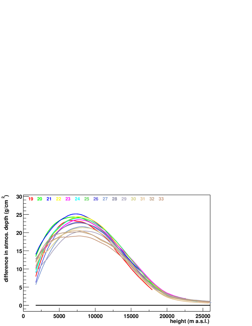
Figure 1: Difference between the US-StdA depth profile and those measured during January/ February 2003, near Malargüe, Argentina.

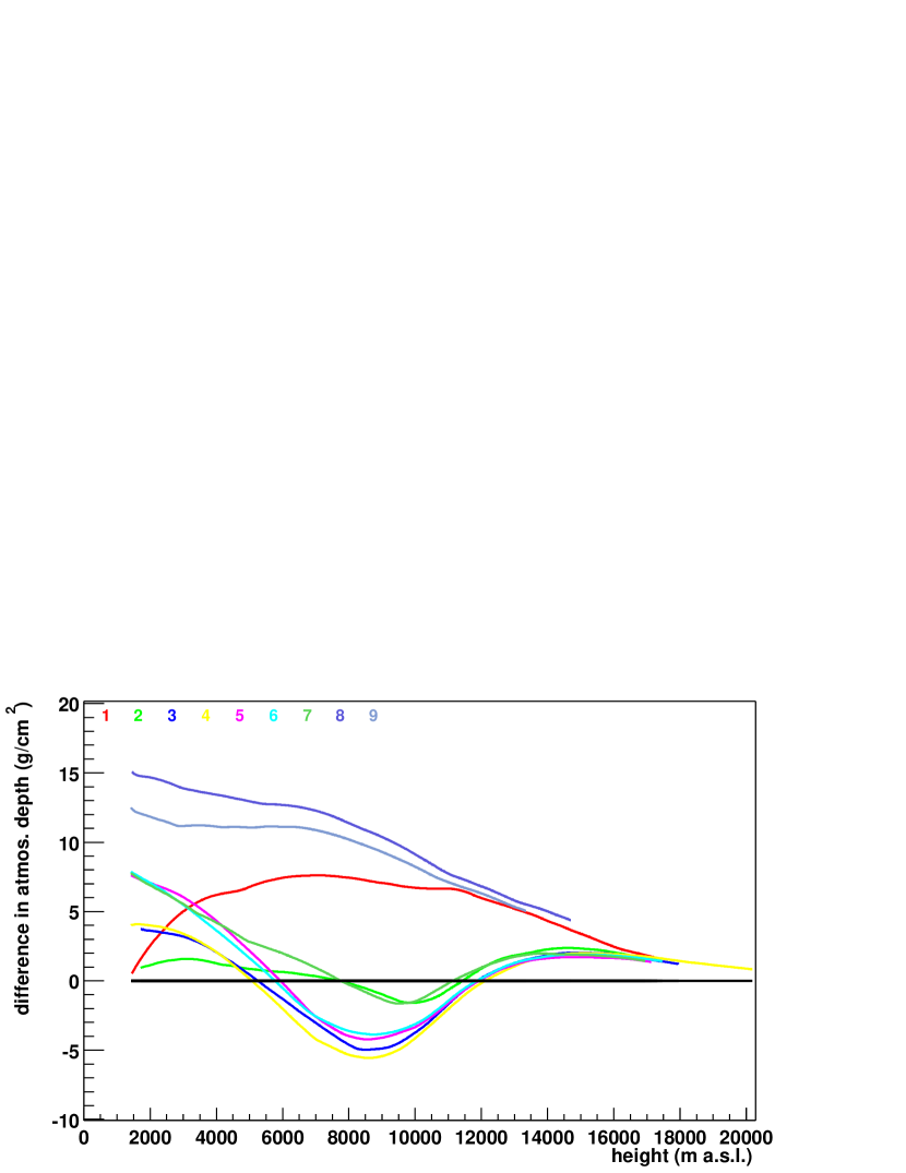
Figure 2: Difference between the US-StdA depth profile and those measured during August 2002, near Malargüe, Argentina.

Atmospheric depth profiles (i.e. atmospheric depths as function of height) were derived for each launch using the previously described procedure. Figs. 2 and 2 show the relative difference between the individual measured profiles and the US-StdA prediction. The launches are consecutively numbered for all campaigns and each line corresponds to one launch. The variation of conditions of the atmosphere within summer was smallest. A representative data set is given in Fig. 2, where the measurements taken during austral summer are shown. During winter, the conditions – in particular those of air pressure and atmospheric depth as the main influencing parameters on the EAS development [15, 18] – differed quite strongly within several days, see Fig. 2.

Atmospheric models were prepared averaging over each season, with the exception of winter. For describing the winter conditions at Pampa Amarilla, two winter models are required. Winter I reflects those situations when air pressure and atmospheric depth are smaller than in the US-StdA at higher altitudes. The five obtained atmospheric models up to 25 km a.s.l. are shown in Figs. 4, 4, and 5, as temperature, pressure, and difference in atmospheric depth profiles, respectively.

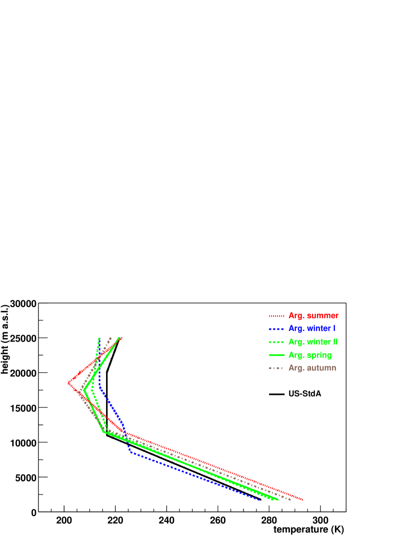
Figure 3: Temperature profiles for averaged seasons at the Pampa Amarilla.

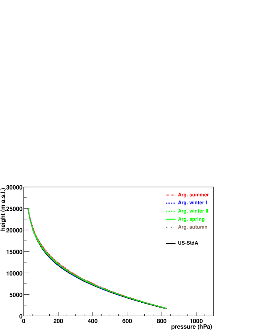
Figure 4: Pressure profiles for averaged seasons at the Pampa Amarilla.

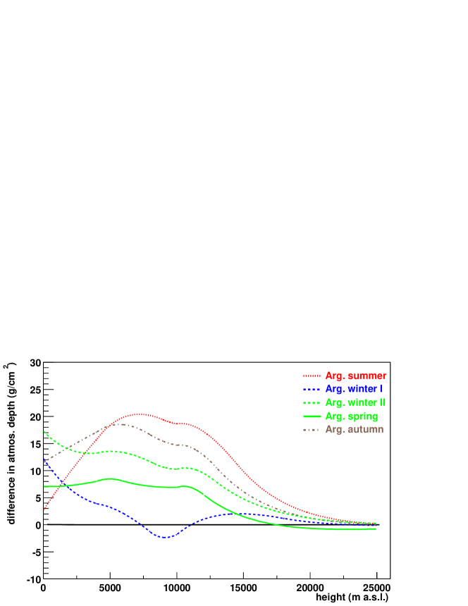
Figure 5: Differences in the average atmospheric depth profiles for the seasons in Argentina according to the US-StdA.

These models are deduced from data of the first five campaigns selecting only clear and calm nights with conditions that would allow operation of fluorescence detectors. For details concerning all radio sounding data see [19]. The corresponding parameters for the atmospheric depth parameterizations are given in the Appendix.

3 Atmospheric Influences on the Reconstruction of Extensive Air Shower Profiles

Fluorescence telescopes detect the longitudinal shower development within a fixed field of view. The visible height range depends on the distance of the EAS to the telescope. For analyzing simulated shower profiles in the geometrical frame of telescopes, these profiles have to be transformed from a description based on vertical atmospheric depth $X_{\mathrm{vert}}$ to geometrical height $h$. However, the development of an EAS depends on the slant atmospheric depth $X$ as the amount of traversed matter which is given by $X=X_{\mathrm{vert}}/\mathrm{cos}\theta$ for zenith angle $\theta$ of the EAS less than 60^∘. Due to this fact, the following discussion depends strongly on the zenith angle of an EAS. For vertical showers, the geometrical conversion effect is smallest.

From the physical point of view, an EAS develops according to the amount of traversed air. Starting with the first interaction of the primary cosmic ray particle, the cascade of secondary particles increases in number of particles as well as in energy deposited in air and fluorescence emission. At the shower maximum, energy losses begin to dominate particle production and the number of particles decreases while propagating further in the atmosphere. The position of the shower maximum in terms of atmospheric depth is closely correlated to the type of the primary particle and is used to identify the cosmic ray for a given primary energy $E_{0}$. Fluorescence telescopes however, observe EAS in terms of geometrical height $h$. Thus, observed profiles have to be converted into atmospheric depth related profiles for an interpretation of the event. As mentioned above, usually the profile of the US-StdA is applied for this purpose.

3.1 Importance of using realistic atmospheric profiles

For this study, 100 iron and 200 proton induced EAS have been simulated using CORSIKA with the hadronic interaction model QGSJET01 [20]. In the following we will use only the average shower profiles calculated from the set of simulations. All showers were generated using the US-StdA and the shower profile is tabulated as function of atmospheric depth. It is sufficient to simulate showers in one atmosphere as the physical development of a shower is only slightly affected by varying atmospheric conditions in terms of changing particle interaction and decay probabilities due to air density distributions. Differences in the observable shower profile as function of altitude are adequately considered by using realistic atmospheric profiles for the conversion of atmospheric depth to geometrical altitude.

This simplified treatment is justified since the shower development depends only very weakly on the used atmospheric depth profile due to different atmospheres. Fig. 6 shows the mean shower profiles of iron induced showers with 10¹⁹ eV and 60^∘ zenith angle. Using two extreme Argentine atmospheres and the US-StdA sets of 100 showers each were simulated. Only very small differences in the shower profile can be observed.

Figure 6: Mean profiles of 100 iron induced showers with $10^{19}$ eV and 60^∘ incident angle in different atmospheres. The simulations were done by implementing the corresponding atmospheric profiles in CORSIKA.

In Fig. 8, the comparison of charged particles of p- and Fe-induced showers with $E_{0}=10^{19}$ eV and $\theta=60^{\circ}$ in the US-StdA can be seen. For this, the underlying simulated EAS in terms of atmospheric depth have been transformed to geometrical height using the parameterization for the US-StdA. Iron induced showers develop earlier and the average position of the shower maximum is reached for the given conditions at $8.4\;$km. Proton induced showers penetrate deeper in the atmosphere and the position of the shower maximum is at $7.6\;$km. The EAS profiles are clearly separated and a discrimination by fluorescence telescope detection is expected.

However, actual atmospheric conditions differ from the US-StdA as shown in Sec. 2. For demonstrating the importance of using a realistic atmospheric profile, we show the same averaged showers in Fig. 8, as they would be observed under two extreme cases of measured Argentine conditions.

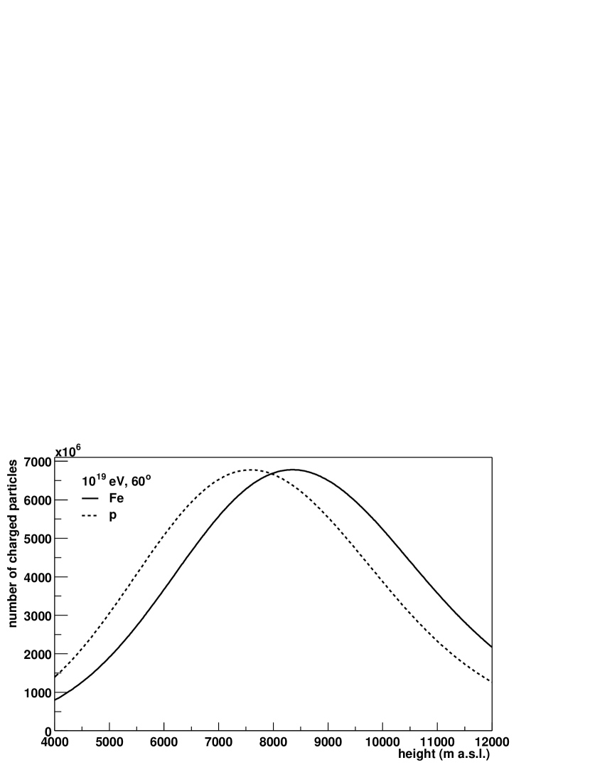
Figure 7: Profiles of charged particles for p- and Fe-induced EAS in US-StdA with 10¹⁹ eV and 60^∘ inclination.

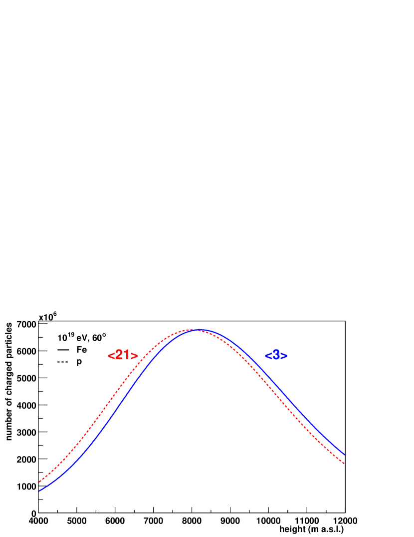
Figure 8: Profiles of charged particles for p-induced EAS in Argentine summer, launch $<$21$>$, and Fe-induced EAS in Argentine winter, launch $<$3$>$, both with 10¹⁹ eV and 60^∘ inclination.

The first case is a night during winter, recorded as radio sounding $\langle$3$\rangle$, and the second case is a night in summer, launch $\langle$21$\rangle$. The accordant atmospheric depths can be seen in Fig. 2 and 2, respectively. This corresponds to the assumption that the deeper penetrating p-induced shower would have been measured in austral summer leading to a shift of longitudinal development towards higher altitudes. The Fe-induced shower is assumed to occur during winter. For these conditions, the positions of the shower maxima of the averaged proton and iron showers are very close together. The shower maximum of the Fe-induced shower in winter is at 8.2 km, that of the p-induced shower in summer is at 8.0 km. Thus the profiles are hardly distinguishable.

Next we consider the number of charged particles in EAS as a function of atmospheric depth $X$. The longitudinal profiles for the simulated p- and Fe-induced EAS in the US-StdA are plotted in Fig. 10. The shown range of the slant atmospheric depth is nearly the same as the range in geometrical altitude given in Figs. 8 and 8. Again, the profiles are clearly distinguishable and the position of the shower maximum for the proton case is at $774\;$g/cm² and for the iron shower at $690\;$g/cm². Adopting the reconstruction point of view, now the EAS profiles in terms of geometrical height are taken as given. The question is how large are the shifts of the shower profiles of Fig. 8 in $X$, if the profiles of actually measured atmospheres are used. Applying atmosphere $\langle$21$\rangle$ to iron induced EAS and $\langle$3$\rangle$ to p-induced showers, the resulting charged particle profiles are plotted in Fig. 10. The position of the shower maximum of the iron shower in atmosphere $\langle$21$\rangle$ would be reconstructed to $735\;$g/cm² and for the p-induced shower to $761\;$g/cm². Relative to US-StdA this corresponds to a shift of about $+45$ g/cm² and $-13$ g/cm² in slant depth for the iron and proton showers, respectively.

Figure 9: Profiles of charged particles for p- and Fe-induced EAS in US-StdA with 10¹⁹ eV and 60^∘ inclination.

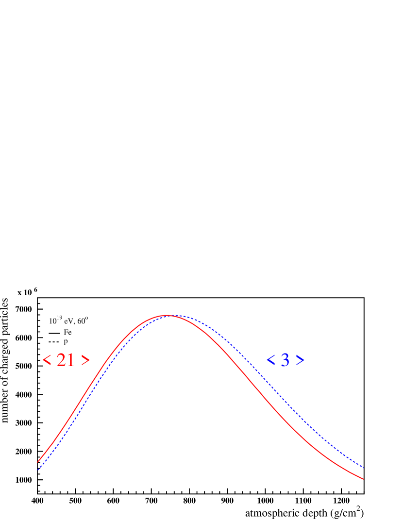
Figure 10: Profiles of charged particles for Fe-induced EAS in Argentine summer, launch $<$21$>$, and p-induced EAS in Argentine winter, launch $<$3$>$, both with 10¹⁹ eV and 60^∘ inclination.

Not only the average position of the shower maximum is indicating the type of the primary particle. Also the width of the distribution of this position for a large number of EAS is systematically different for proton and iron induced showers. The general relation between shower maximum and $E_{0}$ of EAS in the US-StdA can be seen in Fig. 11.

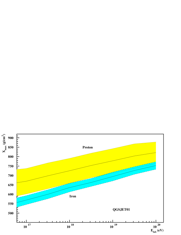
Figure 11: Mean value and fluctuations of the depth of shower maximum for increasing $E_{0}$. The showers were simulated with CORSIKA applying the QGSJET01 hadronic interaction model [20]. For p-induced showers 500 simulations were performed and for Fe-induced 200. The bands denote one standard deviation.

As a concrete example, we show in Fig. 12 the $X_{\rm max}$ distributions of proton and iron induced showers at $10^{19}\;$eV for US-StdA. The fluctuations are much larger and more asymmetric for proton induced showers ($\sigma_{\rm p}\approx$ 60 g/cm²) than for iron induced EAS ($\sigma_{\rm Fe}\approx$ 20 g/cm²).

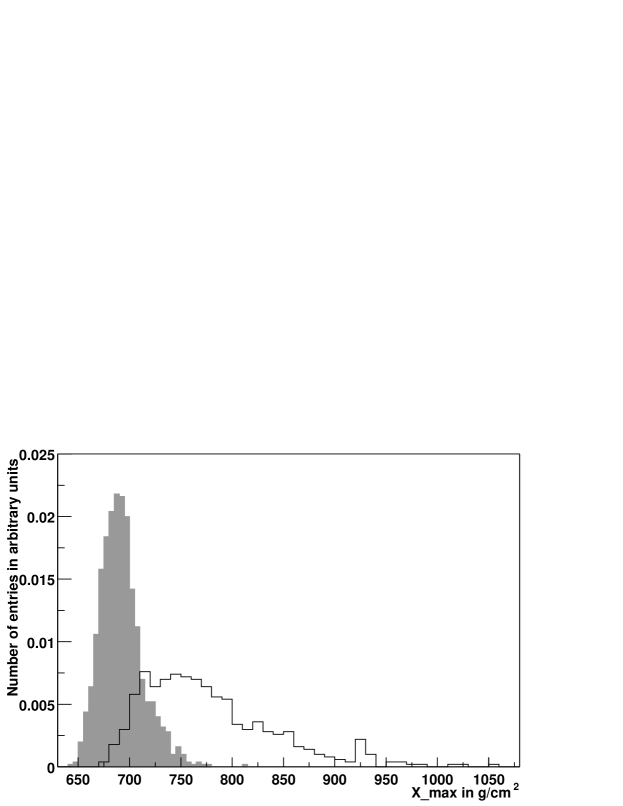
Figure 12: $X_{\rm max}$ distribution for 1000 Fe-induced (shaded histogram) and 500 p-induced (white), 10¹⁹ eV showers given in slant depth.

Some characteristics of these distributions are listed in Table 2.

Table 2: Statistics for the $X_{\mathrm{max}}$ distributions of Figure 12.

	$\mathbf{N_{\mathrm{entry}}}$	Mean	RMS	Minimal Value	Maximal Value
		(g/cm2)	(g/cm2)	(g/cm2)	(g/cm2)
Fe-ind.	1000	692	20.9	644	811
p-ind.	500	778	64.7	671	1056

The information of the width of the distribution of the maximum position of EAS is often used in experiments for deducing the chemical composition of primary cosmic rays from the data [21, 22]. Since for measuring the $X_{\rm max}$ distribution, many EAS events have to be taken into account, however, the atmospheric conditions are different for each event. As demonstrated earlier, the use of the US-Std atmosphere can cause a shift of up to $\sim 40\;$g/cm² for $60^{\circ}$ showers for atmospheric profiles measured at Pampa Amarilla, Argentina. If the local atmosphere above a fluorescence detector changes as much as considered in the extreme examples above on a day-by-day basis, such shifts would considerably broaden the $X_{\rm max}$ distribution of heavier elements. A reconstruction based on a fixed atmospheric profile would lead to a systematic bias towards lighter mass numbers. In the next section, we shall study in detail the influence of different, measured atmospheric conditions on the mean and width of the distribution of the shower maximum.

3.2 Application of averaged seasonal atmospheres for the Pampa Amarilla

First we use our measurements to analyze the atmospheric variations in each season. For two representative altitudes, the corresponding vertical atmospheric depth values obtained with the radio soundings are calculated. In Fig. 14, the distributions of the atmospheric depth for the geometrical height of 8400 m a.s.l. are plotted for different seasons. The height of 8400 m a.s.l. is chosen because it corresponds approximately to the altitude where a Fe-ind. EAS with 10¹⁹ eV and 60^∘ inclination reaches its maximum. The statistics for all four seasons is given in Table 4, admittedly in slant depth underlying a 60^∘ zenith angle. Argentine Summer is marked by a small distribution in contrast to winter. The total width of the distribution for all seasons is 8.2 g/cm² in vertical depth or 16.4 g/cm² in slant depth for the given case. The second example is specified for 2400 m a.s.l., being about the altitude of the shower maximum for a p-ind. EAS with 10¹⁹ eV and vertical incidence. The histogram is shown in Fig. 14 and the statistics is given in Table 4. Again, Argentine summer shows only small variations and at this altitude, Argentine autumn spreads most. However, the width of the distribution for all seasons at this height is only about half the value than for the higher altitude.

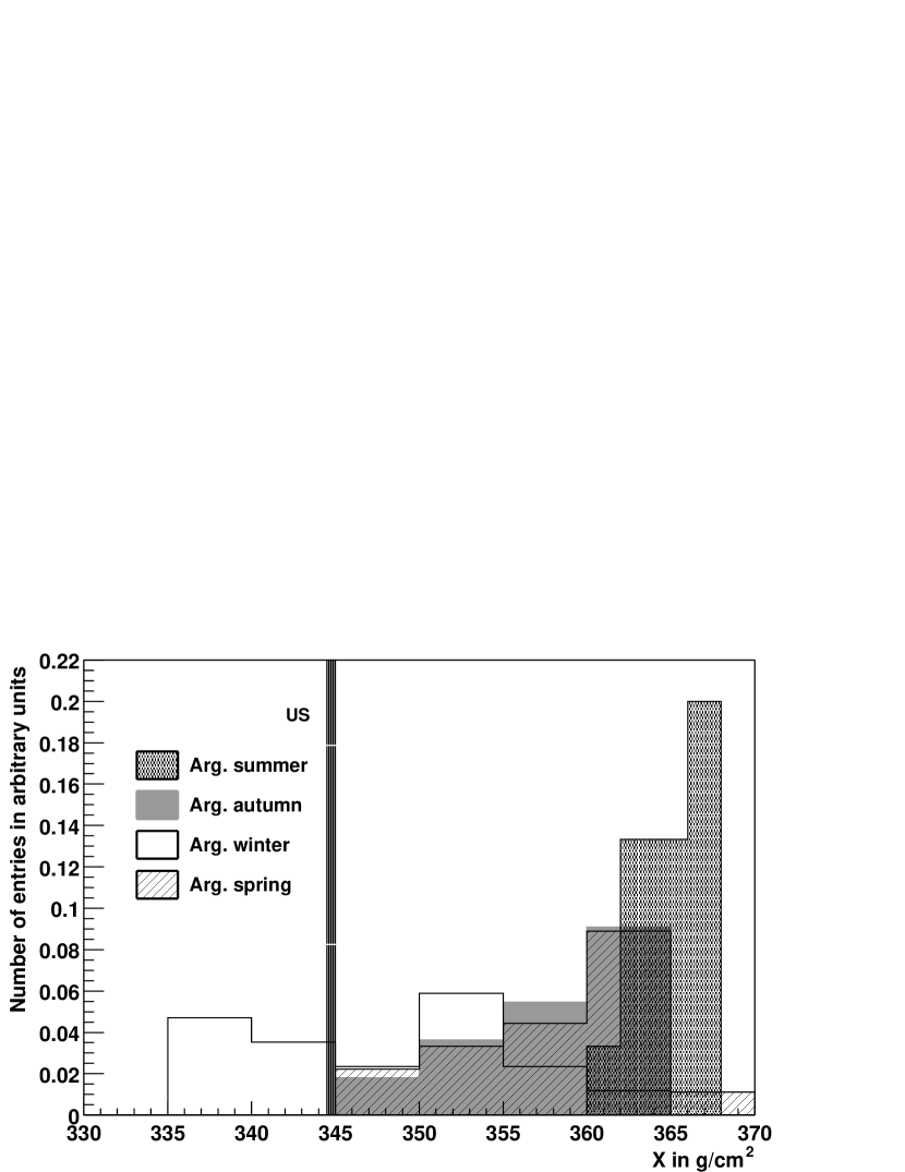
Figure 13: $X$ distribution at 8400 m a.s.l. for the individual profiles measured in Argentina divided into groups by season.

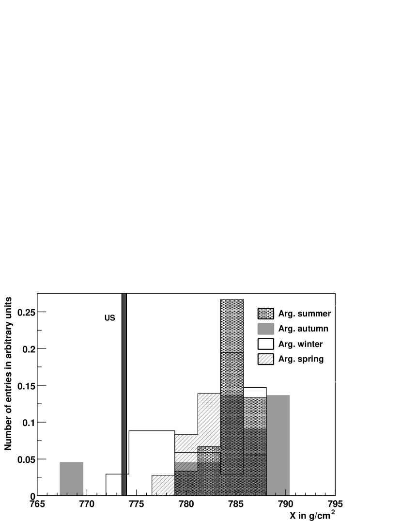
Figure 14: X distribution at 2400 m a.s.l. for the individual profiles measured in Argentina divided into groups by season.

Table 3: Statistics for the slant depth distributions at 8400 m a.s.l. for the individual profiles in Argentina and $60^{\circ}$ zenith angle.

	$\mathbf{N_{\mathrm{entry}}}$	Mean	RMS
		(g/cm2)	(g/cm2)
all	61	714	16.4
Summer	15	730	3.4
Winter	17	696	15.2
Spring	18	716	10.6
Autumn	11	718	9.2

Table 4: Statistics for the slant depth distributions at 2400 m a.s.l. for the individual profiles in Argentina and $0^{\circ}$ zenith angle.

	$\mathbf{N_{\mathrm{entry}}}$	Mean	RMS
		(g/cm2)	(g/cm2)
all	61	783	4.0
Summer	15	785	2.0
Winter	17	781	4.7
Spring	18	783	2.2
Autumn	11	783	5.5

The intrinsic variation of the depth of maximum of proton induced showers is so large that the broadening effect due to the atmosphere becomes negligible. However for iron induced showers, a considerable effect due to atmospheric variations is expected. Additionally, it is obvious that the influence is more important for inclined showers since the slant depth has to be considered for the longitudinal shower development. The difference between US-StdA and the actual atmosphere, as for instance given in Fig. 5, has to be divided by $\mathrm{cos}\theta$, with $\theta$ being the EAS zenith angle. The resulting value represents the shift of the shower profile at each altitude.

The broadening effect of the $X_{\mathrm{max}}$ distribution due to all averaged Argentine seasons and also the shift of the average position of $X_{\mathrm{max}}$ is demonstrated in Tables 5 and 6 for 10¹⁹ eV showers of 60^∘ zenith angle.

Table 5: Statistics for $X_{max}$ distributions for Fe-induced showers with 60^∘ incidence in slant depth.

	$\mathbf{N_{\mathrm{entry}}}$	Mean	RMS	Min. Value	Max. Value
		(g/cm2)	(g/cm2)	(g/cm2)	(g/cm2)
US-StdA	1000	692	20.9	644	811
Arg. averaged	5000	713	26.1	658	851
Arg. Summer	1000	732	21.2	683	851
Arg. Winter I	1000	688	21.4	640	811
Arg. Winter II	1000	715	21.3	666	836
Arg. Spring	1000	706	21.0	658	825
Arg. Autumn	1000	725	21.4	675	846

Table 6: Statistics for $X_{max}$ distributions for p-induced showers with 60^∘ incidence in slant depth.

	$\mathbf{N_{\mathrm{entry}}}$	Mean	RMS	Min. Value	Max. Value
		(g/cm2)	(g/cm2)	(g/cm2)	(g/cm2)
US-StdA	500	778	64.7	671	1056
Arg. averaged	2500	800	67.3	667	1094
Arg. Summer	500	818	64.7	710	1094
Arg. Winter I	500	777	66.7	667	1062
Arg. Winter II	500	802	65.7	693	1083
Arg. Spring	500	792	65.1	685	1073
Arg. Autumn	500	812	65.9	703	1093

Regarding all seasons, the average shift of the position of the shower maximum is 21 g/cm² for the Fe-ind. shower and 22 g/cm² for p-ind. These number could also be extracted from Fig. 5. The average difference in atmospheric depth $\Delta X$ according to the US-StdA is about 10 g/cm² at $\approx$ 8 km a.s.l. For these examples of 60^∘ inclined showers, it results into a shift in slant depth of $\Delta X/\mathrm{cos}\theta\approx$ 20 g/cm². For each season, the number can be obtained in the same way. The numbers for the variation of the $X_{\mathrm{max}}$ distribution indicate only small atmospheric effects within each season. However for the average of all seasons, the atmospheric conditions affect the variation especially in the case of iron. The distribution becomes wider for about 25% for iron but only 4% for p-ind. showers compared to the distribution in the US-StdA.

For the sake of completeness it should be mentioned that the shift of the average $X_{\rm max}$ position is correspondingly half of the values above for vertical showers. The width of the distribution is unaffected. The numerical values for the different seasons can be taken from Fig. 5. In this case the broadening is negligible for all primaries considered here.

4 Summary and Conclusion

The importance of using realistic atmospheric depth profiles, strictly speaking air density profiles, for reconstructing the longitudinal shower development has been investigated. The depth of shower maximum has been considered in detail since it is often used for identifying the type of the primary particle. Applying atmospheres measured at site of the southern Pierre Auger experiment, two main effects are observed with regard to using the US standard atmosphere parameterization for data analysis and simulation studies. First of all, atmospheric conditions differing from the US-StdA can lead to a significant, systematic shift of the position of the shower maximum. Secondly, the distribution of the depth of maximum due to intrinsic shower fluctuations is broadened by temporal variations of the atmospheric conditions.

The importance of atmospheric variations depends on the shower angle and primary particle. The more inclined an air shower is the more important is the detailed knowledge of the atmospheric profile. For vertical EAS, the influence of atmospheric profile variations can be nearly neglected, but for incidence angles larger than 40^∘, the use of the US standard atmosphere biases the interpretation of extensive air showers. Showers induced by heavy particles are more sensitive to atmospheric profile deviations than that of light primaries.

This investigation is based on meteorological data obtained at the Pampa Amarilla, Argentina, where the southern part of the Pierre Auger Observatory is situated. However, it is expected that the atmospheric density profiles are as important for other fluorescence air shower experiments as for the Auger experiment. This is supported by Fig. 15, in which deviations of the atmospheric depth profiles relative to the US-StdA are shown for two extreme profiles measured in Germany. The curve for summer is very similar to Argentine summer and the deviation in winter even exceeds that of the Argentine winter.

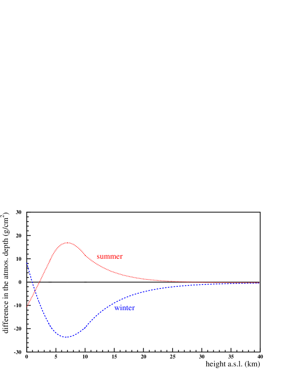
Figure 15: Difference in the atmospheric depth in g/cm² from the Stuttgart, Germany, summer / winter atmosphere to the US-StdA [23].

Seasonal atmospheric depth profiles have been developed for the southern Auger detector. With the exception of Argentine winter, each season can be described by a typical shape of the atmospheric profile. Although the individual measurements correlate for the other seasons well with seasonally averaged atmospheric conditions, day-to-day variations are significant. Currently our investigations are limited by the statistics of radio soundings. We will continue to measure the molecular atmosphere at the Pampa Amarilla and plan to develop atmospheric models for various time scales.

Forthcoming articles of this series will study the impacts of using realistic temperature and pressure profiles on the fluorescence yield and on the transmission due to Rayleigh scattering of the fluorescence light. In both cases, a wavelength dependent analysis has to be performed. Similar analyses have also be done for the impact on the atmospheric Cherenkov technique [24]. Only minor effects – in addition to corrections for the variations of the atmospheric ground pressure – are expected for the observation of EAS using particle detectors at ground.

Appendix: Parameterizations of the Atmospheric Depth

Table 7: Parameters of the US-StdA [13].

Layer $i$	Altitude $h$	$a_{i}$	$b_{i}$	$c_{i}$
	(km)	(g/cm2)	(g/cm2)	(cm)
1	0 … 4	-186.5562	1222.6562	994186.38
2	4 … 10	-94.919	1144.9069	878153.55
3	10 … 40	0.61289	1305.5948	636143.04
4	40 … 100	0.0	540.1778	772170.16
5	$>$ 100	0.01128292	1.	109

For CORSIKA versions 5.8 (release August 1998) and higher, it is possible to read in external atmospheric models. This option enables not only the change of the parameters but also the variable selection of the boundaries for the four lowest layers.

Table 8: Parameters of the average Argentine winter I atmosphere.

Layer $i$	Altitude $h$	$a_{i}$	$b_{i}$	$c_{i}$
	(km)	(g/cm2)	(g/cm2)	(cm)
1	0 … 8	-150.247839	1198.5972	945766.30
2	8 … 18.1	-6.66194377	1198.8796	681780.12
3	18.1 … 34.5	0.94880452	1419.4152	620224.52
4	34.5 … 100	4.8966557223$\cdot 10^{-4}$	730.6380	728157.92
5	$>$ 100	0.01128292	1.	109

Table 9: Parameters of the average Argentine winter II atmosphere.

Layer $i$	Altitude $h$	$a_{i}$	$b_{i}$	$c_{i}$
	(km)	(g/cm2)	(g/cm2)	(cm)
1	0 … 8.3	-126.110950	1179.5010	939228.66
2	8.3 … 12.9	-47.6124452	1172.4883	787969.34
3	12.9 … 34	1.00758296	1437.4911	620008.53
4	34 … 100	5.1046180899$\cdot 10^{-4}$	761.3281	724585.33
5	$>$ 100	0.01128292	1.	109

Table 10: Parameters of the average Argentine spring atmosphere.

Layer $i$	Altitude $h$	$a_{i}$	$b_{i}$	$c_{i}$
	(km)	(g/cm2)	(g/cm2)	(cm)
1	0 … 5.9	-159.683519	1202.8804	977139.52
2	5.9 … 12	-79.5570480	1148.6275	858087.01
3	12 … 34.5	0.98914795	1432.0312	614451.60
4	34.5 … 100	4.87191289$\cdot 10^{-4}$	696.42788	730875.73
5	$>$ 100	0.01128292	1.	109

Table 11: Parameters of the average Argentine summer atmosphere.

Layer $i$	Altitude $h$	$a_{i}$	$b_{i}$	$c_{i}$
	(km)	(g/cm2)	(g/cm2)	(cm)
1	0 … 9	-136.562242	1175.3347	986169.72
2	9 … 14.6	-44.2165390	1180.3694	793171.45
3	14.6 … 33	1.37778789	1614.5404	600120.97
4	33 … 100	5.06583365$\cdot 10^{-4}$	755.56438	725247.87
5	$>$ 100	0.01128292	1.	109

Table 12: Parameters of the average Argentine autumn atmosphere.

Layer $i$	Altitude $h$	$a_{i}$	$b_{i}$	$c_{i}$
	(km)	(g/cm2)	(g/cm2)	(cm)
1	0 … 8	-149.305029	1196.9290	985241.10
2	8 … 13	-59.771936	1173.2537	819245.00
3	13 … 33.5	1.17357181	1502.1837	611220.86
4	33.5 … 100	5.03287179$\cdot 10^{-4}$	750.89705	725797.06
5	$>$ 100	0.01128292	1.	109

Table 13: Parameters of the US-StdA obtained with the method applied in this work, for details see [19].

Layer $i$	Altitude $h$	$a_{i}$	$b_{i}$	$c_{i}$
	(km)	(g/cm2)	(g/cm2)	(cm)
1	0 … 7	-149.801663	1183.6071	954248.34
2	7 … 11.4	-57.932486	1143.0425	800005.34
3	11.4 … 37	0.63631894	1322.9748	629568.93
4	37 … 100	4.35453690$\cdot 10^{-4}$	655.67307	737521.77
5	$>$ 100	0.01128292	1.	109

References

- [1] R. M. Baltrusaitis et al., Nucl. Instr. and Meth. in Phys. Res. A240, 410, (1985)
- [2] C. C. Jui et al. (HiRes Collab.), in Invited Rapporteur and Highlight Papers, Proc. 26th Int. Cos. Ray Conf. (Salt Lake City), 370, (2000)
-
[3]
A. Etchegoyen et al., FERMILAB-PUB-96-024,
http://www.auger.org/admin/DesignReport/, (1996) - [4] J. Blümer (Pierre Auger Collab.), J. Phys. G29, 867, (2003)
- [5] J. Abraham el al. (Pierre Auger Collab.), Nucl. Instr. and Meth. in Phys. Res. A, Vol. 523, Issue 1, 50, (2004)
-
[6]
M. Fukushima et al. (TA Collab.),
http://www-ta.icrr.u-tokyo.ac.jp/TA, (2000) - [7] M. Fukushima, Prog. Theor. Phys. Suppl. 151, 206, (2003)
- [8] L. Scarsi et al., http://www.euso-mission.org/
- [9] A. Petrolini (EUSO Collab.), Nucl. Phys. Proc. Suppl. 113, 329, (2002)
- [10] M. Pallavicini (EUSO Collab.), Nucl. Instr. and Meth. in Phys. Res. A502, 155, (2003)
- [11] F. Kakimoto et al., Nucl. Instr. and Meth. in Phys. Res. A372, 527, (1996)
- [12] National Aeronautics and Space Administration (NASA), U.S. Standard Atmosphere 1976, NASA-TM-X-74335, (1976)
- [13] D. Heck et al., CORSIKA: A Monte Carlo Code to Simulate Extensive Air Showers, Report FZKA 6019, Forschungszentrum Karlsruhe, (1998)
- [14] S. J. Sciutto, Auger technical note GAP-99-020, (1999)
- [15] B. Keilhauer et al., Proc. 28th Int. Cos. Ray Conf. (Tsukuba), 2, 879, (2003)
- [16] Dr. Graw Messgeräte GmbH & Co., Nürnberg, http://www.graw.de
- [17] B. A. Bodhaine et al., J. Atmos. Ocean. Tech., Vol. 16, 1854, (1999)
- [18] B. Wilczyńska et al., Proc. 28th Int. Cos. Ray Conf. (Tsukuba), 2, 571, (2003)
-
[19]
B. Keilhauer, Investigation of Atmospheric Effects on the
Development of Extensive Air Showers and their Detection with the Pierre Auger
Observatory, Report FZKA 6958, Forschungszentrum Karlsruhe, (2004);
Auger technical note GAP-2003-107, (2003) - [20] N. N. Kalmykov, S. S. Ostapchenko, A. I. Pavlov, Nucl. Phys. B (Proc. Suppl.) 52B, 17, (1997)
- [21] J. W. Cronin, TAUP 2003 proceedings, astro-ph/0402487, (2004)
- [22] A. A. Watson, astro-ph/0312475, (2003)
-
[23]
H. Ulrich, Untersuchung atmosphärischer Einflüsse auf die Entwicklung
ausgedehnter Luftschauer anhand von Simulationsrechnungen, Diploma thesis, University of
Karlsruhe, (1997) (unpublished);
H. Ulrich et al., Auger technical note GAP-98-043, (1998) - [24] K. Bernlöhr, Astropart. Phys. 12, 255, (2000)