The Lyman- Forest Power Spectrum from the Sloan Digital Sky Survey
Abstract
We measure the power spectrum, , of the transmitted flux in the Ly forest using 3035 high redshift quasar spectra from the Sloan Digital Sky Survey. This sample is almost two orders of magnitude larger than any previously available data set, yielding statistical errors of % and on, respectively, the overall amplitude and logarithmic slope of . This unprecedented statistical power requires a correspondingly careful analysis of the data and of possible systematic contaminations in it. For this purpose we reanalyze the raw spectra to make use of information not preserved by the standard pipeline. We investigate the details of the noise in the data, resolution of the spectrograph, sky subtraction, quasar continuum, and metal absorption. We find that background sources such as metals contribute significantly to the total power and have to be subtracted properly. We also find clear evidence for SiIII correlations with the Ly forest and suggest a simple model to account for this contribution to the power. While it is likely that our newly developed analysis technique does not eliminate all systematic errors in the measurement below the level of the statistical errors, our tests indicate that any residual systematics in the analysis are unlikely to affect the inference of cosmological parameters from . These results should provide an essential ingredient for all future attempts to constrain modeling of structure formation, cosmological parameters, and theories for the origin of primordial fluctuations.
1 Introduction
Although the Ly forest was discovered many decades ago (Lynds, 1971), it has only recently emerged as one of the prime tracers of the large scale structure in the Universe. The high resolution measurements using the Keck HIRES spectrograph (Vogt et al., 1994) have been largely reproduced using hydrodynamical simulations (Cen et al., 1994; Zhang et al., 1995; Hernquist et al., 1996; Theuns et al., 1998) and semi-analytical models (Gnedin & Hui, 1998). The picture that has emerged from these studies is one in which the neutral gas responsible for the absorption is in a relatively low density, smooth environment, which implies a simple connection between the gas and the underlying dark matter. The neutral fraction of the gas is determined by the interplay between the recombination rate (which depends on the temperature of the gas) and ionization caused by ultraviolet photons. Photoionization heating and expansion cooling cause the gas density and temperature to be tightly related, except where mild shocks heat up the gas. This leads to a tight relation between the absorption and the gas density. Finally, the gas density is closely related to the dark matter density on large scales, while on small scales the effects of thermal broadening and Jeans smoothing must be included. In the simplest picture described here, all of the physics ingredients are known and can be modeled. The fact that one can trace the fluctuations over a range of redshifts ( using ground based spectrographs) and over a range of scales, which are typically smaller than the scales of other tracers, is the main strength of this method. It becomes particularly powerful when combined with cosmic microwave background (CMB) anisotropies or other tracers that are sensitive to larger scales. Such a combination is sensitive to the shape of the primordial spectrum of fluctuations, which is one of the few observationally accessible probes of the early universe. These observations are therefore directly testing the models of the early universe such as inflation.
Ly forest observations and constraints on cosmology have been explored by several groups in the past. Most of the analyses focused on the power spectrum, , of the fluctuations in the Ly forest flux,
| (1) |
where is the optical depth to Ly absorption. The first such work was by Croft et al. (1998), followed by McDonald et al. (2000), Croft et al. (2002), and Kim et al. (2003). These groups were limited to a few dozen spectra at most. Recent theoretical analyses, in addition to above, have been performed by Gnedin & Hamilton (2002), Zaldarriaga et al. (2001), and Seljak et al. (2003). In the latter two of these papers the degeneracy between the amplitude and slope of the primordial power spectrum and the normalization of the optical depth-density relation [most sensitive to the intensity of UV background, and typically parametrized in terms of the mean transmitted flux fraction, ] was emphasized, which leads to a significant expansion of the allowed range of cosmological parameters relative to what one would have inferred from the errors on the flux power spectrum alone. Seljak et al. (2003) have shown that the current Ly forest constraints are consistent with the CDM model favored by recent CMB data, testing it in a regime of redshift and length scale not probed by other measurements, but that within the CDM framework they do not add much leverage on parameter values beyond that afforded by the CMB data alone.
An important practical implication of the theoretical breakthroughs of the 1990s is that large scale structure in the Ly forest can be effectively studied with moderate resolution spectra. Once the spectrum is modeled as a continuous phenomenon rather than a collection of discrete lines, there is no need to resolve every feature. Some of the studies cited above use high resolution (Å) spectra, some use moderate resolution () spectra, and some use a mix of the two.
The goal of this paper is to present a new measurement of the Ly forest power spectrum, based on Sloan Digital Sky Survey (SDSS; York et al. (2000)) spectra that probe the Ly forest at a resolution (Å FWHM). This sample is almost two orders of magnitude larger than anything that was available before. As such it greatly increases the statistical power of the Ly forest, making it comparable to the CMB from WMAP. At the same time, the required tolerance of systematic errors also increases by the same amount. This requires a careful investigation of all of the sources of systematic errors, and a large portion of this paper is devoted to the issue of possible systematics in the data and their influence on the parameters of interest. We also discuss how the analysis we perform and results we obtain differ from what can be done using the standard spectral pipeline outputs in the public SDSS data. In part because of the practicalities of work in a large, multi-institutional collaboration, and in part because of the importance of obtaining an accurate measurement with well understood statistical and systematic errors, the Ly forest power spectrum has been pursued by two independent groups within the SDSS, one led by P. McDonald and U. Seljak, and the other by L. Hui and A. Lidz. The methods employed are different and have been developed independently. Results of the alternative analysis will be presented elsewhere (Hui et al., in preparation).
We only present the observational measurement of the SDSS Ly forest power spectrum in the current paper. Independent of any theoretical interpretation, this basic result should be robust on the scales for which we give results, , where if is the wavelength of a Fourier mode (not to be confused with spectral wavelength), here measured in (note that throughout the paper we frequently use velocity in place of observed wavelength, with the understanding that all that enters into our calculations are velocity differences between pixels of measured spectra, defined by – we do not measure power on scales large enough for the imperfections in this expression to become relevant). The choice of -range is determined by the continuum fluctuations on the low end and spectral resolution at the high end. We note also that the useful range is limited not only by these uncertainties, which are related to the data analysis, but also by the uncertainties in the theoretical modeling and/or additional astrophysical effects. We will address these latter issues in more detail in a separate publication. However, we do not completely decouple the theory from the data analysis. For example, when discussing the importance of systematic errors it is useful to understand how they would affect cosmological results like the slope and amplitude of the matter power spectrum, so much of our discussion of systematics is devoted to this issue.
The common usage of the term Ly forest is to describe the Ly absorption by neutral hydrogen in the relatively low density bulk of the IGM. In this paper we include damped-Ly systems (DLAs) in the definition of the “forest”, so it includes all HI-Ly absorption. We could try to remove DLAs before measuring , because they are more difficult to simulate than the lower optical depth absorption; however, we believe the advantage of removal is illusory. If the DLAs were located randomly within the IGM (which they certainly are not completely), it would be simple to include them in the theory using their known column density distribution. If they are not located randomly, the regions obscured by DLAs in the spectra are special, so the effect of removing the DLAs still must be understood using simulations. We leave the handling of the effects of DLAs as a problem for the theory, which we will address elsewhere.
Absorption by metals is also difficult to simulate accurately, so we would like to remove this contribution to . This is relatively easy to do for transitions with wavelength Å, but it is basically impossible for transitions with , because the metal features always appear mixed with HI-Ly. We will subtract the power measured in the rest wavelength range Å from our measurement of the power in the forest, which removes the effect of transitions with longer wavelength, but we leave shorter wavelength transitions as part of the forest. The only significant contaminant of this kind that we can identify is SiIII absorption at Å, and we develop a simple and effective way to account for this in the theory. We refer to our final background-subtracted power spectrum as , and use for the raw power measured in the interval . We are using the range Å for the Ly forest.
The outline of this paper is as follows. In §2, we describe the selection of our data set and the preparation of spectra for the measurement of . In §3 we describe the method used to measure the power spectrum and estimate the error bars, test the procedure, and give the basic results. We perform consistency checks on the results and discuss systematic errors in §4, which is followed by a brief recipe for using our results in §5, and conclusions in §6.
2 Data Selection and Preparation
We describe the sample of quasar spectra that we use in §2.1. In §2.2 we explain how we remove broad absorption line (BAL) quasars from the sample. In §2.3 we explain how we combine spectra from different exposures for the same quasar and use the differences between exposures to understand the noise in the data. We discuss the resolution of the spectra in §2.4. Finally, in §2.5 we describe how we divide each spectrum by an estimate of the quasar continuum, the expected mean absorption level in the spectrum, and a spectral calibration vector (see below), to produce the vectors of transmission-fluctuation estimates, , for each quasar, from which we will measure .
2.1 SDSS Observations and Sample Selection
The Sloan Digital Sky Survey (York et al., 2000) uses a drift-scanning imaging camera (Gunn et al., 1998) and a 640 fiber double spectrograph on a dedicated 2.5 m telescope. It is an ongoing survey to image 10,000 sq. deg. of the sky in the SDSS AB magnitude system (Fukugita et al., 1996; Stoughton et al., 2002) and to obtain spectra for galaxies and quasars. The astrometric calibration is good to better than rms per coordinate (Pier et al., 2003), and the photometric calibration is accurate to 3% or better (Hogg et al., 2001; Smith et al., 2002). The data sample used in this paper was compiled in Summer 2002 and is a combination of data releases one (Abazajian et al., 2003) and two (Abazajian et al., 2004).
About 13% of the spectroscopic survey targets are quasar candidates selected based on their colors (Richards et al., 2002). The magnitude limit for UV-excess objects is , while additional high-redshift candidates () are targeted to . Fibers are allocated according to a tiling algorithm (Blanton et al., 2003), with the galaxy sample and the quasar sample being the top priorities. The remaining 8% of fibers serve for calibration purposes.
SDSS spectra are obtained using plates holding 640 fibers, each of which subtends 3 on the sky; the spectra cover . The pixel width is a slowly varying function of wavelength, but is typically . The resolution also varies, but is typically also rms (i.e., the resolution is and there are pixels per FWHM resolution element). All quasars have multiple spectra, usually taken one after the other (timescales of a fraction of an hour), so the quasar variability can be ignored (in the opposite case it would act as an additional source of noise). The co-added spectra in the official SDSS release use local spline interpolation onto a uniform grid of pixels of width , and do not guarantee the noise to be uncorrelated. We therefore redo this step starting from the individual exposures. This is discussed in more detail below. Spectral flux errors per pixel in most cases are about erg s-1 cm-2 Å-1. Redshifts are automatically assigned by the SDSS spectral classification algorithm, which is based on fitting of templates to each spectrum (Schlegel et al., in preparation).
We limit ourselves to quasars with redshift when measuring the power in the Ly forest region of spectra, so that each spectrum contains a significant stretch of the Ly forest above the detector cutoff at 3800 Å (which corresponds to Ly absorption at ). We use the sample compiled in Summer 2002, cut down to 3035 spectra by eliminating some plates of questionable quality, some spectra where two different redshift estimation codes disagree, and some BAL quasars (see below). Figure 1 shows the redshift distribution of the data.
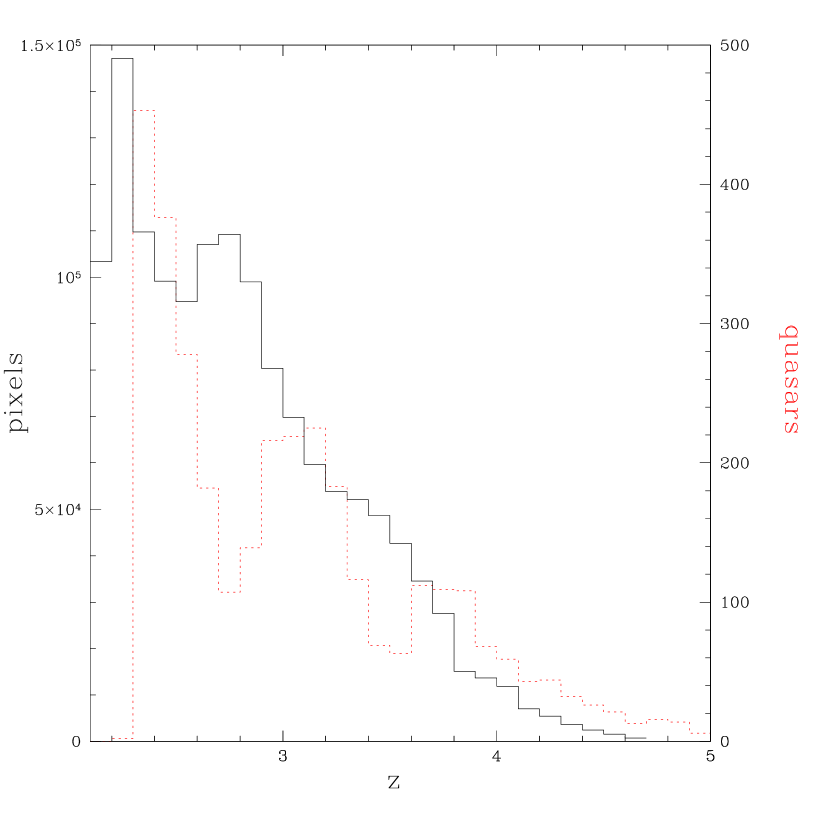
The dashed, red histogram shows the distribution of quasar redshifts. The solid, black histogram shows the distribution of pixels in the range Å. Note that there is a gap in the quasar redshifts around , which is due to the stellar locus crossing the quasar locus in the 5-color SDSS photometry (Richards et al., 2002). Figure 2 shows an example SDSS spectrum of a quasar.
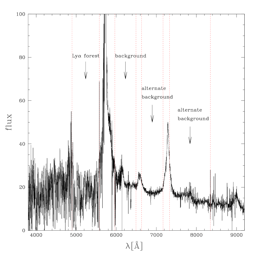
This spectrum is unusual in that most have lower S/N, and most quasars are at lower redshift.
We employ an additional sample of spectra with , so that we can study the full observed wavelength range, , outside the confusion of the Ly forest. As we discuss in §3.4, we compute a non-negligible background power term (probably mostly metal absorption), by measuring the power in the wavelength range Å. Using only the primary sample, we would not be able to compute this term for observed wavelengths below Å.
We remove several wavelength regions from our analysis because of calibration problems: Å, Å, Å, Å, and Å (the last two have no direct effect on the results we present). Most of these problems are due to strong sky lines.
2.2 BAL Removal
Our sample was initially examined by eye, and the most extreme broad absorption line (BAL) quasars were removed (see Hall et al. (2002) for a discussion of BALs). When we first measured the background power in the region Å, we found that the most extreme outliers in power were still obvious BALs (this was not true of the Ly forest region). To test the importance of these systems to our Ly forest power measurement, we removed a further 147 quasars using the following automated method: Each spectrum is smoothed by a Gaussian with rms width . The continuum within the region Å is redefined by dividing by the mean flux-to-continuum ratio in the region. A quasar is identified as a BAL quasar if the region Å contains a long continuous set of pixels that all fall more than 20% above or below our estimated continuum (we initially identified wide regions with flux above the continuum out of simple curiosity, but found that these are in practice almost always obvious BAL quasars where the continuum has been biased low by the BAL feature). We iterate the continuum redefinition twice, computing the new mean after throwing out pixels more than 20% below the previous mean, but this makes almost no difference to the results. Note that the smoothing was applied to allow easier identification of BALs in noisy spectra. As we show below, this BAL cut makes essentially no difference to our result, although it does have a noticeable effect on the power measurement in the region Å.
2.3 Combining Exposures and Calibrating the Noise
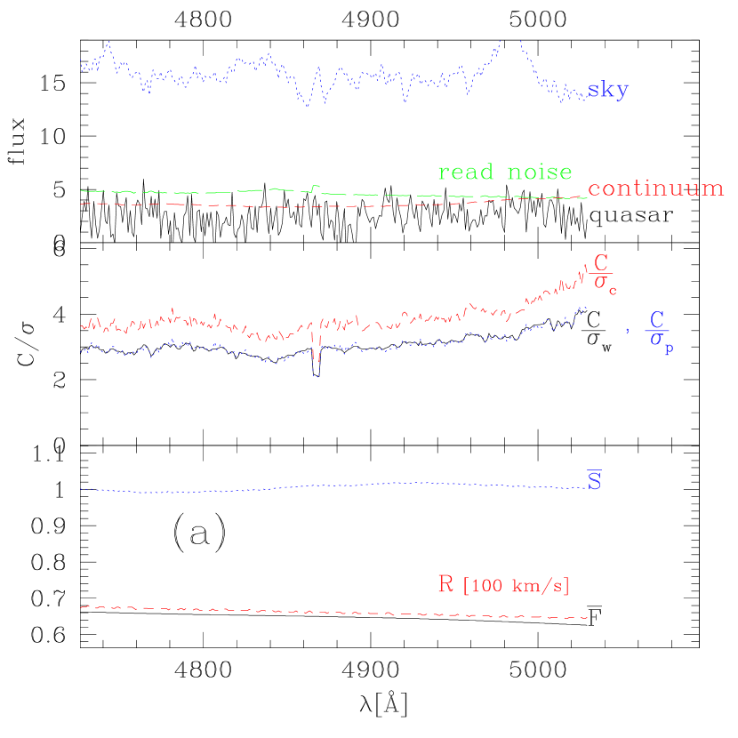
SDSS obtains multiple (at least 3) exposures for each quasar. We combine the individual exposure spectra to produce a single spectrum, using a nearest-grid-point method that produces uncorrelated noise and a reasonably well-defined sampling window. For each pixel we record estimates of wavelength, quasar flux, resolution, sky flux, read-noise, and two different total noise estimates. The first noise estimate, which we will call simply ( for pipeline), is computed using the error array given for the exposure spectra by the spectral reduction pipeline. The second noise estimate, which we call ( for component), is computed by summing the read-noise and the noise implied by estimates of the number of photons corresponding to the quasar flux and sky flux. The two noise estimates generally do not agree, but this is not a problem for us because we ultimately recalibrate the noise (next). Finally, we record for each pixel, computed by treating the determination of the combined flux value for each pixel as a one parameter fit to the measurements given by the different exposures. Examples of the more important of these quantities in Ly forest regions are shown in Figure 3.
![[Uncaptioned image]](/html/astro-ph/0405013/assets/x4.png)
![[Uncaptioned image]](/html/astro-ph/0405013/assets/x5.png)
For comparison to the sky and quasar flux levels, we have converted the Gaussian read-noise into the flux of photons that would contribute the same noise variance. Several elements of Figure 3 (e.g., the estimation of the quasar continuum and ) will be described later in this paper.
The noise estimate from the standard SDSS pipeline is only approximate. The accuracy of the noise estimate required for our purpose is much higher than anticipated when the pipeline was developed. For this reason we use the differences between single-exposure spectra for the same quasar to determine the noise properties of the data. We construct difference spectra by combining the flux-calibrated exposures with alternating sign for each exposure, i.e., we use exactly the same procedure that we normally use to produce combined spectra from the exposures, except half of the exposures are subtracted instead of added, so the mean result is zero (we drop the last exposure when there are an odd number – this is not the most efficient method possible, but we do not need it to be). The result is a direct measure of the exposure-to-exposure changes. We measure the power spectrum of these difference spectra using the method described in §3.1, including noise subtraction based on the pipeline noise estimates for the pixels. The result is shown in Figure 4 (points with error bars).
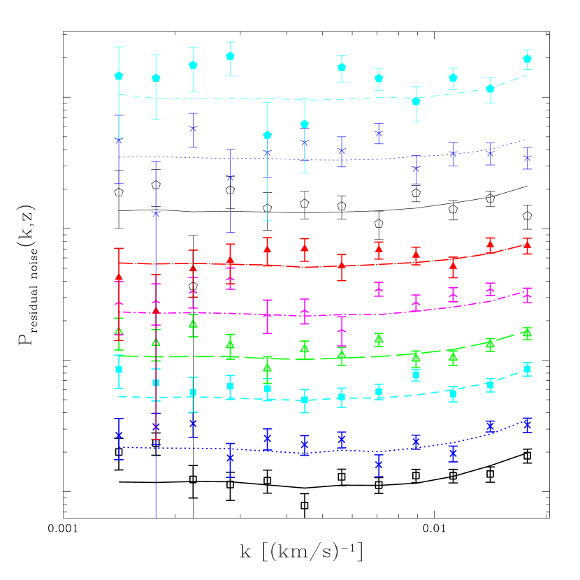
We obtain a clear detection of power, where there should be none if the spectra differ only by the noise estimate from the pipeline which is being subtracted. If we assume that the noise has been underestimated by a constant factor, and fit for that factor using the error covariance matrix estimated by bootstrap resampling, we find a decent fit: for 107 degrees of freedom (formally, this fit is not good because is unlikely to be this high by chance). This fit uses our usual points in . The best fit value of the excess noise contribution is % of the original noise estimate, indicating that the rms noise was underestimated by 8%. The best fit and goodness of fit do not change if we add points on larger scales. The quality of the fit begins to degrade as we add points with larger , but the best fit value changes by only 1% (in power) out to the Nyquist frequency of the data. Of course, we have no reason to expect a single redshift-independent factor to describe the relation between the true and pipeline noise, so the formally bad is not a fundamental problem. We check for systematic change with redshift by allowing a power law dependence, , but find no significant detection (). Our final method will effectively account for evolution anyway, as described below.
A dependence different than expected for white noise could be a problem for us, so we check for this by fitting for a power law dependence, [with ], finding , a significant detection ( is now a reasonable 123.3 for 106 dof). Allowing a running of the power law, , does not improve the fit (). The slope we find corresponds to a % change in 16% of the noise power at the extremes of our range, i.e., only % of the total noise power, which is a relatively small fraction of the Ly forest power except at the highest (see Figure 11 below). We henceforth assume that the extra noise is proportional to rather than white (this makes % difference in the final results except for the one highest , lowest point where the difference is 2%).
How accurate is this noise estimate based on differences between exposures? Our difference spectra will contain a component of the Ly forest power if the calibration between exposures is not perfect. The power in this term would be suppressed relative to the Ly forest power by the fractional calibration error squared, so it would be very small unless the exposure-to-exposure calibration errors were quite large. The fact that a simple one parameter extra-noise model fits reasonably well, in the face of variation in redshift, noise amplitude, and , argues against calibration errors being a big problem. More convincingly, we measure nearly the same excess noise contribution (%) and slope () in the region Å as we do in the Ly forest. This argues against any connection to leaking Ly forest power. Note that the effective absolute level of noise in the Å region is about half that in the Ly forest region, so this test shows that the fraction of extra noise does not depend strongly on the noise level itself.
Pixels in different exposures are not perfectly aligned, and misalignment can allow Ly forest power to leak into our difference spectra. To test this alternative explanation for the apparent excess noise in the spectra, we split the spectra into two groups with approximately equal weight, based on the rms misalignment in the forest region (the alignment is known from the wavelength calibration of the exposures, which is thought to be practically perfect). We find the same excess noise power in both the poorly aligned group (%, ) and the better aligned group (%, ), suggesting that the excess power is not due to misalignment. Furthermore, the presence of a similar level of excess noise power outside of the forest region again argues against leakage. We therefore believe that our noise estimate is considerably more accurate than the noise estimate from the SDSS pipeline.
In our initial power spectrum analysis we multiplied the noise-power estimated from the pipeline errors by the factor 1.16 for all spectra; however, when we split the data based on the mean value of for the exposure combination (see §4.4) we found that the large and small subsamples disagreed significantly on the results. We eliminated this problem by estimating the noise-correction factor individually for each spectrum, by fitting to the power in the difference spectrum for that quasar. The mean extra power from these fits is still close to 16%, but there is considerable scatter. When we use these individual estimates, the correlation between measured and disappears, i.e, the mean value of for a spectrum’s exposure combination was a good indicator of the amount by which the noise in each spectrum was misestimated. Note that there are statistical errors in these noise estimates for each spectrum, of the same order as the error for which we are trying to correct; however, there is no systematic bias associated with these errors, and the random error they contribute is automatically included in our final bootstrap errors. In fact, including the spectrum-by-spectrum noise estimate reduces the bootstrap errors slightly on small scales, verifying that these estimates are on average more accurate than the original noise estimates. It is not known why the noise is misestimated by the standard pipeline. Tests at this level have not been done before.
Our final data product will be a measurement of binned in and , i.e., a matrix where labels bins with and labels bins with . We will also give the noise power that was subtracted, , in the same bins. We suggest allowing a 5% rms freedom in the noise amplitude in each bin when performing model fits, i.e., for each bin subtract from , and add to . This is probably overly conservative for any one bin, but implies a combined freedom (for 9 bins) on an overall noise misestimation. This seems prudent, even though it is not really required by any test we have performed.
2.4 Accuracy of the Resolution
The resolution of the SDSS spectra is estimated using lines from calibration lamps mounted on the telescope structure. Shifts of the detector pixel grid relative to a fixed observed wavelength frame during an exposure, which we will call flexure, are expected to be the dominant source of error in this spectral resolution estimate. We tried estimating the rate of shifting for each pixel by differencing the wavelength calibrations of adjacent exposures (this calibration is determined very precisely for each exposure using the positions of sky lines). The implied extra smoothing only changes the power by % at our highest bin.
The strong sky line at 5577 Å provides a good opportunity to measure the resolution more directly (note that the spectral wavelengths are in vacuum, and heliocentric, so this and other sky lines generally appear shifted from their standard wavelength). We measure the power spectrum in sky spectra in the range Å. If the sky line has negligible width and the smoothing has a Gaussian shape with rms width , the power spectrum should be proportional to , where is the pixel width (the pixelization effect is subdominant but not negligible). In Figure 5 we show the measured power averaged over all the sky spectra after dividing each individual measurement by , where and are the local values (they are to a good approximation constant over the range we are looking at), and also dividing each measurement by the value at a low where the resolution should not have any effect.
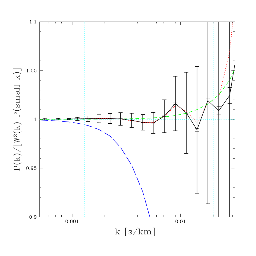
The result is remarkably close to unity, indicating that the estimated resolution is an accurate representation of the true resolution. What are the small wiggles? Figure 6 shows an example of the region we Fourier transform to measure the power.

We believe the small features to the sides of the main line are OH lines at 5564 and 5589 Å (Slanger et al., 2003). We test this explanation for the wiggles by constructing mock sky spectra that simply have a delta function at 5579Å and two more with 0.003 times the main line’s amplitude at 5566 and 5591 Å, convolved with the resolution and pixelization (0.003 was chosen to give the best fit to the wiggles). The red, dotted line in Figure 5 shows the same resolution test using the mocks. We see that the wiggles are essentially perfectly reproduced. In conclusion: the resolution profile appears to be perfectly Gaussian, with exactly the width expected from the given resolution. There is apparently no room for even a 2% level effect from flexure. We are prevented from performing the same kind of measurement using other sky lines by similar features which are always much larger relative to the central line.
We suggest that fits to include a multiplicative uncertainty on the overall power, of the form , where is a single parameter in the fit subject to the rms constraint . This allows for a % change in the smoothing kernel at our highest , similar to our estimate of the error from flexure. This error estimate is somewhat arbitrary, but the evidence we have presented suggests that it should be smaller, so our estimate is conservative.
Note that this resolution test, and the noise calibration, cannot be used directly with the standard pipeline spectra, where the exposures are combined in a different way. The reader may be confused at this point about how our spectra differ from the standard publicly available set, so we give the following summary:
-
•
Our nearest-grid-point combination of the exposures produces uncorrelated noise in pixels (to the extent that the noise in the exposures was uncorrelated, which is expected from the way they are extracted), while the standard pipeline uses a local splining procedure which does a good but not perfect job of preventing noise correlation.
-
•
When combining exposures we record the effect of different pixel sizes, misalignment of the pixels, and flexure of the detector during exposures, which can influence the effective resolution.
-
•
We record the contribution of quasar flux, sky flux, and read-noise to the total noise in each pixel. Knowing the contribution from quasar flux is important if pixel-by-pixel noise weighting is to be used, because the correlation between flux level and noise amplitude can lead to biases (see the end of §2.5).
-
•
We correct for the bias in the exposure combination associated with cross-correlation between the noise variance level in exposure pixels and the quasar flux in the pixel (a different incarnation of the problem alluded to in the previous point).
-
•
The noise is recalibrated for each spectrum by differencing the exposures. The noise variance in the standard pipeline exposure spectra is underestimated by on average 16%, on top of any error related to the exposure combination, and the power measured in the difference spectra is slightly tilted relative to white noise.
The last point is the most important.
2.5 Determination of the Continuum and Mean Absorption Level
Our goal is to measure the power spectrum of the fluctuations in the transmitted flux fraction through the IGM, , where and is the Ly forest optical depth (as defined in §1). However, the spectrum of each quasar is the product of and the quasar continuum (note that we use “continuum” to refer to all the flux emitted by the quasar, including emission lines), further complicated by errors in the detector calibration and absorption by longer wavelength transitions. The details of the procedure we use to separate these contributions will be presented elsewhere, here we give the basic idea and key results that are relevant for the flux power spectrum determination.
We use an iterative procedure to determine the components of the data model
| (2) |
where is the raw flux in pixel , is the noise, is the overall normalization of the quasar spectrum, is the mean quasar continuum shape, are fluctuations around the mean continuum, is a mean generalized calibration vector (this includes wavelength dependent calibration errors in the SDSS spectra, but also the mean absorption by metal lines with resonance wavelength Å), are fluctuations around , such as individual metal lines or variable calibration errors, is the mean Ly forest absorption at a given redshift, and are the fluctuations in Ly forest absorption. Note that here, as most places in this paper, is the redshift of gas that would produce Ly absorption in the pixel, not the redshift of the quasar. Briefly, we determine for each spectrum, the global functions , , and , and a set of principal component analysis (PCA) eigenvectors that describe by, in turn, computing each component of the model from all the spectra while holding all the others fixed. E.g., is estimated in bins of by averaging over all the pixels in the Ly forest that fall in each bin. We separate from by measuring in the rest wavelength range Å, i.e., outside the Ly forest. A few iterations suffice to determine all the components of the model independently. Three examples of the results are shown in Figure 3. The full details of this procedure will be presented in a separate paper focused on a precise determination of .
In preparation for measuring the power spectrum, we divide each quasar spectrum by our estimate of . The power in the and terms is completely negligible (always % of and usually much less). are represented for each quasar by N PCA eigenvectors. We have tried several different values for N ranging from 0 to 13, and find that the power spectrum results depend slightly (but not critically) on the value, as we discuss below. For our final results we use , i.e., we only divide by a mean continuum, although we will also show how using affects the cosmological fit results. We do not use the PCA continua because we are not satisfied with their robustness, and division by them frequently actually increases the resulting power slightly. This may indicate that the error introduced by allowing additional freedom in the continuum is larger than the continuum fluctuations that we are trying to remove. Our study of PCA continua was primarily aimed at determining rather than the power spectrum, so we cannot be certain that the PCA method could not be used productively in a power spectrum measurement if it was more carefully optimized for that application. Because we know that our continuum estimate (which involves an extrapolation from outside the Ly forest region) is not perfect within the Ly forest, we further divide each chunk of spectrum that will be used to make a power spectrum estimate by its mean (optimally computed considering both observational noise and absorption variance). We call our resulting observed data vector , where is the normalized noise fluctuation and we are ignoring the cross-terms between , , and . As we describe in detail below, is treated as a random noise background and its statistical properties are determined by measuring the power spectrum in the rest wavelength range Å, where (and ).
A small but non-negligible detail of our procedure is hidden within our description of the normalization of the spectra. When we estimate the mean to divide by, we weight the computation optimally using the covariance matrix, , of the pixels ( is discussed in more detail in our explanation of the power spectrum measurement below). includes Ly forest fluctuations and measurement noise. We do not use our best estimate of the measurement noise directly for the weighting, because the noise variance estimate is correlated with the measured flux in the pixel, which leads to a bias: the mean is underestimated because lower flux pixels have lower noise. The original noise estimate is , where is the flux from the quasar, is the flux from the sky, and accounts for the conversion between the units of flux and photons (this description is slightly idealized since the reduction of two-dimensional CCD data to a spectrum introduces some complications). To remove the correlation between flux and noise, we subtract from and add , where . We call the final result ( for weight; see Figure 3 for some comparisons of the noise estimates). The estimate of we have from the spectral reduction pipeline is not perfect, so our replacement of the correlated part of the noise amplitude is imperfect. We make a final, very small, correction to the mean estimation based on a direct computation of the cross-correlation between the flux and noise amplitude. We use the same decorrelated noise amplitudes for weighting the power spectrum extraction (discussed below); however, the bias is completely insignificant in that case (i.e., computed using the original noise estimates for weighting is practically identical).
3 Power Spectrum Determination
The high precision of the measurement obtainable using the SDSS data sample requires unprecedented (in this field) care in the design and testing of the procedure used to produce it. We describe the basic method that we use to extract a power spectrum and estimate the errors in §3.1. In §3.2 we present the test of the full method as implemented in our code, using mock data sets. In §3.3 we give the raw result for the measurement of power in the Ly forest region.
We aim to measure the power spectrum of , representing the correlation of fluctuations in the Ly forest absorption only; however, the covariance matrix of the data vector is
| (3) |
(the three components of as we have defined it should be uncorrelated). The noise term in equation (3) is relatively easy to compute and subtract. We estimate and subtract most of by defining
| (4) |
where is always defined by , so that we are subtracting power measured in the same observed wavelength ranges, not the same quasar spectrum (we remind the reader that we have defined to mean the power measured in the range ). As it appears in , is the redshift of gas that would produce Ly absorption in this part of the quasar spectrum, if it was not at a higher redshift than the quasar, i.e., is really just an indicator of observed wavelength. The subtraction in equation (4) will completely remove the power due to transitions with Å, including SiIV (a doublet absorbing at rest wavelengths 1393.75 and 1402.77 Å) and CIV (another doublet at 1548.20 and 1550.78 Å). Note that this subtraction of metal power is exact, not an approximation [except for the approximation that ], because we are determining the metal power in exactly the same observed wavelength range as the Ly forest power from which it is being subtracted, i.e., the same gas, at the same redshift, is doing the absorbing both inside and outside the forest, so the absorption will have identical statistical properties. This background subtraction will also remove any strictly observed-wavelength-dependent power introduced by the detector, such as spectrum to spectrum variations in the calibration of the detector. We implement it in §3.4.
3.1 Core Method
In this subsection we describe our method for extracting the power spectrum, , from any selected rest wavelength range (§3.1.1), and estimating its statistical uncertainty (§3.1.2).
3.1.1 Band-Power Estimation
We estimate using the quadratic estimation method, which is essentially a fast iterative implementation of the maximum likelihood estimator (we follow the expressions as given in Seljak (1998)). This method is optimal for a Gaussian probability distribution. While the power spectrum estimates are not Gaussian distributed, the deviations are small, as shown below. We measure the power in flat bands with edges given by where ranges from 0 to 30 (to produce 29 bands), although we will not give results for some of the large and small-scale bands when we think they are unreliable. Defining , where are the fluctuations we are measuring (e.g., within the forest) and are the normalized noise fluctuations, a band-power estimate, , for each chunk of spectrum is given by
| (5) |
where , , , ,
| (6) |
is the Fisher matrix and the noise bias is
| (7) |
Note that we could include the background power explicitly in these equations as a noise source when measuring the power in the Ly forest region, but we ignore this because its contribution is too small to change the weighting significantly. We will subtract it from the estimates later. The noise subtraction term, , is computed using the pipeline noise estimates, (not ), with the amplitude corrected as discussed above based on the differences between exposures. In principle, in these equations should be the true covariance matrix; however, as we discuss below, we use the measured covariance from a previous iteration of the power spectrum determination instead.
Except in a few cases that we will identify as they arise, when we set out to measure the power in a defined rest-wavelength region (e.g., Å for the Ly forest region) we first use equation (5) to estimate the power separately in halves of the region in each spectrum (e.g., Å and Å). Our choice of half-spectra is a compromise between competing desires for resolution in redshift and wavenumber. The full length of the forest in a spectrum corresponds to a redshift interval, , that is unnecessarily large. While the precision of the measured power spectrum would support smaller than half-spectrum chunks to give finer redshift resolution than , the shorter chunks would limit the -space resolution. Note that we could have used full chunks and still achieved the same -resolution by more carefully applying the estimator equation, as we discuss below, but this would increase the computational time without much improvement in the final errors on the scales of relevance.
After computing estimates for each half-spectrum, we perform a weighted average to determine in redshift bins centered at where (in this paper we only present results up to ). Each bin is the average of the power in all the half-spectra for which the redshift of the central pixel falls within of the bin center (we discuss below how we correct for an asymmetric distribution of data within a bin). We combine sets of estimates using the Fisher matrices (equation 6) for the weighting. In practice this means that we sum the quantity in parentheses in equation (5) over all estimates and multiply the result by the inverse of the sum of the Fisher matrices for each individual estimate. Our procedure would be optimal for Gaussian data, which the Ly forest is not; however, when we use the Gaussian approximation to compute the errors on the measured power the results are not much different from the more accurate bootstrap errors (see §3.1.2), so we conclude that our method is not far from optimal.
Whenever we have a finite length of spectrum, there will be mixing between the power in different bins. Variable noise or gaps in the data will produce more mixing. This mixing is described in terms of a window matrix, which is given by the Fisher matrix in equation 6. In our standard procedure, the power spectrum estimates in equation 5 are multiplied with the inverse of Fisher matrix and are thus deconvolved with the window, which removes the mixing of other modes into the bin one is estimating (however, the bins are still correlated). This method thus produces a diagonal window matrix, so each combined estimate of represents exactly the range of corresponding to its bin. Our tests below show that there is no practical problem with instability in the Fisher matrix inversion (the window matrices are close to diagonal to begin with). A diagonal window matrix is desirable from a theoretical standpoint because our ability to compute the power spectrum from simulations is limited at both low (by limited box size) and high (by simulation resolution and complexity of physics). In the few cases where we use the power without deconvolution, we are using the estimator , where (Seljak, 1998).
To compute the weight matrix , we need an estimate of , i.e., the power spectrum we are trying to measure. We solve this problem by computing iteratively. The first estimate is made assuming . In subsequent iterations we compute from the previous estimate of . This procedure converges quickly (the difference between and a reasonable estimate of is significant, but once is in the right ballpark it does not matter what it is exactly). We add a large constant (10.0) to all elements of the weight matrix, to remove all direct sensitivity of our power measurement to the mean of the chunk. This makes very little difference to the results on the scales we present. We are however still sensitive to the mean estimate from when we divided the spectrum by it. Even if the mean estimates are correct on average, the statistical error on the mean for each spectrum can still lead to a bias. If the errors on the mean estimate were small and uncorrelated with the fluctuations in the flux field, the bias would be , where is the error on the mean [to lowest order in , i.e., the bias is , where is the fractional error in the mean, and ]. We divide each estimate by this factor as part of our standard procedure; however, as we discuss below when we test our code on mock spectra, this approximation is not sufficient and we will need to include another small, -dependent, factor determined numerically using the mock spectra (this is the only use of the mock spectra other than for testing).
The reader may at this point be wondering what redshift the resulting should be taken to represent, i.e., is not necessarily the center of weight of the data, and neither is the mean redshift of the pixels in the bin, considering the rather complicated weighting in equation (5). In fact, the effective redshift is not even the same for each -bin in the same -bin. We resolve this question – represents the power spectrum at precisely (to first order) – in our construction of and , where and label pixels at redshifts and , and labels the redshift bin in which this chunk of spectrum falls. To account for the evolution from and to , we define a power spectrum growth factor, , where
| (8) |
(we use a one-sided derivative estimate instead of equation 8 for the first and last redshift bins). Now , where and is computed as if the pixels were located at the center of the bin. Finally, . This correction may be difficult to understand intuitively at first, but it is really quite simple. The modification of just corrects the power spectrum estimate for the excess (dearth) of power that we expect for pixels in the high (low) redshift ends of the bin. The correction to affects the weighting, simply producing a more accurate at the redshift of the pixels in question.
Note that an alternative method would be to treat the points as simply parameters of a continuous power spectrum defined by some form of interpolation. This would mean would have non-zero derivative with respect to more than one of the power spectrum bins (e.g., usually two for linear interpolation). This method would be elegant, and probably produce narrower effective window functions in the direction; however, it will increase the correlation in the direction between measurement errors, because the same pixels would contribute to more than one power spectrum point. Since this more sophisticated method would allow long chunks of spectra to be used without degrading our resolution, it would be most useful if we were trying to measure the power on even larger scales.
How does our method compare to the straightforward Fourier transform (FT) method? The basic FT method is to project the data vector, , onto a set of modes of the form , and to simply compute the variance of the amplitudes of all the modes with in some bin, i.e.,
| (9) |
where and define the bin, and the discrete spacing of is somewhat arbitrary (the natural spacing is , where is the length of the spectrum, but nothing prevents one from choosing more finely spaced s). Our estimator, equation (5), can be cast in a similar form, i.e., as a projection of the data vector onto a set of modes, and a sum of the squares of the mode amplitudes. We require that the mode amplitudes are statistically independent, which makes their computation equivalent to a computation of Karhunen-Loève eigenmodes (see, e.g., Tegmark et al. (1997)). Figure 7 shows the two most important modes for our bin with , for the chunk of spectrum shown in Figure 3a.
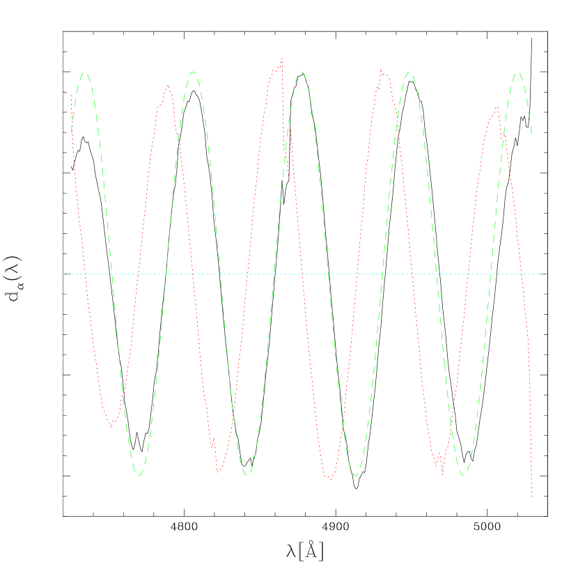
In this case two modes differing primarily by a phase shift, analogous to and , contain most of the information, because our bin width is approximately . We see that the difference between our modes and a simple sine wave is not dramatic – there is a little bit of edge tapering (downweighting the edges to make the effective window on the data more compact in Fourier space) and some straightforward downweighting of the most noisy pixels. Curiously, there seems to be an additional effect where pixels adjacent to an edge are given extra weight, possibly as a way of compensating for missing data (this is seen more clearly in spectra where a narrow gap is present in the middle of the data). The picture is similar for bins with larger , except of course that there are increasingly many important modes as the width of our bins increases (the bins have a fixed width , but the relevant mode width is ). For more discussion of the quadratic estimator see, e.g., Tegmark (1997).
The method we adopt is optimal for Gaussian fields and therefore guarantees that no other method can surpass it. An additional advantage is that within this formalism window and covariance matrices are automatically computed. For continuous spectra with few gaps and near uniform noise one does not necessarily expect an FT method to be significantly worse. In practice the noise level is slowly varying across the spectrum, so averaging all the pixels uniformly is not optimal and degrades performance. Another advantage is that with our method each pixel pair has its own effective redshift and the correlations for a given pair are then interpolated to the redshift of interest using the appropriate evolution. In the FT method the whole spectrum is Fourier transformed first, so the redshift information is preserved only in an averaged sense, but a priori it is not clear how this average is defined.
3.1.2 Bootstrap Error Estimation
While the Fisher matrix obtained during the estimation process would give the error matrix for if the data were Gaussian, we cannot reliably assume this. Our solution is to compute a bootstrap error matrix by the standard procedure (Press et al. 1992). From our data set of spectra, we form a bootstrap data set by selecting spectra at random, with replacement. The covariance matrix of is taken to be , where , is an estimate of the power in the th bin from a bootstrap data set, and means average over bootstrap realizations. We generally use 4000 realizations, after checking that this produces convergence in the result. We assume that the error correlations extend only one bin off diagonal in the direction, because the spectrum of a single quasar practically never contributes to non-adjacent bins.
We have no compelling reason to believe that this method of computing the error bars will give rigorously correct results. Considering the large number of off-diagonal elements that must be estimated, one worry is that a particular linear combination of the bins may accidentally vary very little in our data set, so it will appear to have an unrealistically small error. Our tests on mock spectra (§3.2.2) show no sign of this problem. Still, to be conservative we apply one tweak to after it is computed, in an attempt to inoculate it against the possibility. We perform a singular-value decomposition on , which produces a set of independent vectors and their variances. We then compute the variances of the same vectors under the Gaussian approximation, using the Fisher matrix. If the bootstrap variance is smaller than the Gaussian variance we replace it with the Gaussian variance. Finally, we transform back to . The tests on mock samples described below give us confidence that our procedure is reliable.
3.2 Tests on Mock Data Sets
We validate our procedure as implemented in code by applying it to mock data sets. Many iterations of these tests were required to produce results that show no serious problems in the error estimation or the power spectrum estimation itself. Testing the results on realistically created mock data is absolutely essential for measurements of such high precision. In §3.2.1 we describe our procedure for generating the mock spectra. We test our bootstrap error estimates in §3.2.2. Finally, we test the power spectrum estimation procedure for systematic errors in §3.2.3.
3.2.1 Generating Mock Spectra
We generate mock spectra by combining the auxiliary information we have for each observed spectrum (e.g., our continuum estimate, noise estimate, sky estimate, etc.) with a simplified version of the Bi et al. (1992) model for the field, which results in realistic looking spectra.
For each observed quasar we start with the term we divide by before computing the power spectrum, (see equation 2). We multiply this by (generated as described below), smooth the result using the resolution from the observed spectrum, and sample the result onto the observed grid of pixels. This produces a noise free version of the flux we would observe coming from this quasar. We add flux from the sky as estimated for the observed spectrum, and transform the total flux to the number of photons that would be expected in each pixel. We generate a Poisson deviate with this mean, add the appropriate Gaussian read-noise for each pixel, transform back to the original flux units, and subtract the sky flux estimate to obtain an observed (noisy) quasar spectrum. The results of this procedure for each observed quasar are written into files in the same format as the observed spectra, so exactly the same code can be used to measure the power in the mock spectra.
To generate the fields we use a simple model that is arranged to give roughly the correct power spectrum as a function of and , and the correct mean absorption as a function of redshift. For each observed spectrum, we start by generating a Gaussian random field, , on a very long, relatively finely spaced grid (65536 cells with width , to be precise), with power spectrum
| (10) |
where , , and [this was chosen after some experimentation because it produces a final flux power spectrum with approximately the same dependence as the observed ]. An arbitrary cell in this grid is chosen to correspond to the redshift of the quasar, and the evolution of the amplitude of the power spectrum with redshift is imposed by the transformation with , where the form of was chosen so that the final flux power spectrum would evolve like the observed one. Next we make the squared lognormal transformation , where is computed from the input power spectrum, including the amplitude factor (the factor in the exponential just fixes the mean of the lognormal field to 1). We smooth the field with a Gaussian filter with rms width and multiply it by a factor to produce a field (this redshift evolution factor produces roughly the observed redshift evolution of ). The mock transmitted flux in each grid cell is then , which is sampled as described above.
The procedure described above leads to realistic looking spectra of the Ly forest. We have verified that it generates a bispectrum that is within a factor of 2 of the one measured in N-body simulations. The main advantages of this procedure over the N-body simulation approach when generating the mock spectra are that it is faster, so one can make an arbitrary number of independent realizations, and that the simulated spectra can be of arbitrary length, important to eliminate any periodicity effects (this would be impossible with simulations, where a typical box size is much shorter than the total length of a single spectrum). Both of these advantages are critical for a high precision test. We determine the true by a simple FFT of extremely long fields (without redshift evolution).
3.2.2 Tests of the Error Estimates
Without accurate statistical errors it is difficult to identify systematic problems, so we first test our bootstrap procedure for estimating the errors. Note that there is no reason to expect bootstrap errors to be perfect (there is even some ambiguity in how exactly the bootstrapping should be done when the data do not consist of statistically identical objects). Regardless of systematic errors in the method, the only difference between the power spectra measured from two mock data sets that differ only in the random seed that was used to create them should be the statistical errors that we estimate. We test our error bars by generating ten different sets of mock data and computing for the differences between each of them and their error weighted mean, using the bootstrap error bars and the 108 points in , and . This is effectively a fit of 108 parameters to 1080 data points, with 972 degrees of freedom. The total is 939, perfectly consistent with a random fluctuation around the mean, and strongly disfavoring an underestimation of the errors by more than a couple percent.
3.2.3 Tests of the Power Estimates
We can now search for systematic errors. To enhance the statistical significance of any errors, we average our ten sets of mock spectra to form a single, more precise measurement. The result is shown in Figure 8.
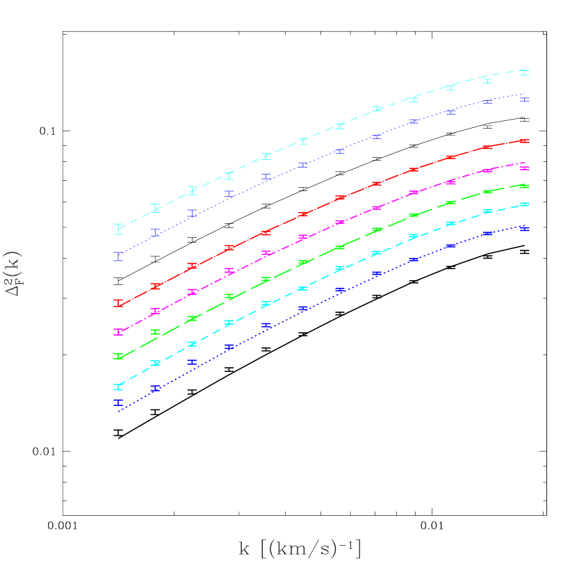
The results look reasonably good; however, we find an unacceptably bad for the comparison between our measured and the true power spectrum (there are 108 degrees of freedom). To quantify the systematic problem, we first assume the bias has the form and fit for the values of and that minimize in the comparison. We find and with for 106 degrees of freedom [the pivot point was chosen to make the errors independent; the amplitude coefficient would be larger if we were not already dividing by as explained in §3.1.1]. The combination of slope and amplitude errors corresponds to a 3.1% excess of power at our largest scale, , and a 1.3% underestimate at . We find some less significant dependencies by generalizing the fitting formula even more to
| (11) |
where , with . The parameters are , , , , and , with . Where does this bias come from? We expect some bias related to the division of each chunk of spectrum by its overall mean (not because of an integral constraint suppression of large-scale power – our estimator should take care of that – but because of statistical error in the estimate of the mean that we divide by). When we measure the power without this division by the mean, which we can only do using mock spectra, we find significantly smaller corrections – small enough to ignore when model fitting.
We expect that this bias should be present when we use real observed spectra, so we will correct for it by dividing the measured power by . We describe its effect on the amplitude and slope of the power spectrum below (table 1).
3.3 Raw Power
Figure 9 shows the raw power measured in our standard Ly forest rest wavelength range, .
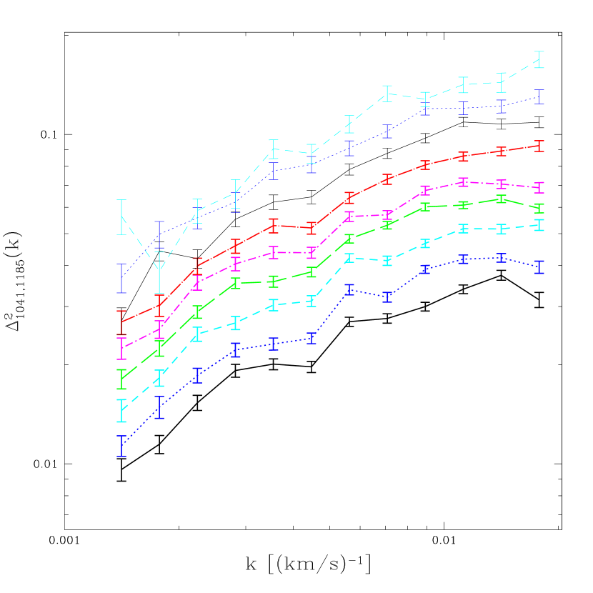
All the figures in this subsection show , not the background subtracted power . Our normalization convention is:
| (12) |
We usually plot the dimensionless quantity , the contribution to the variance per unit .
Figure 10 shows the fractional errors on all of the measured points.
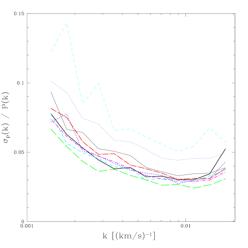
The errors are less than 5% for most of the points, and frequently as small as 3%. If we were only estimating a single amplitude parameter by combining all these points then its error would be 0.6%. An overall logarithmic slope would have an error . The errors on the largest scales are increased somewhat by the diagonalization of the window matrix.
Figure 11 shows the ratio of subtracted noise power to measured signal power () for each point.
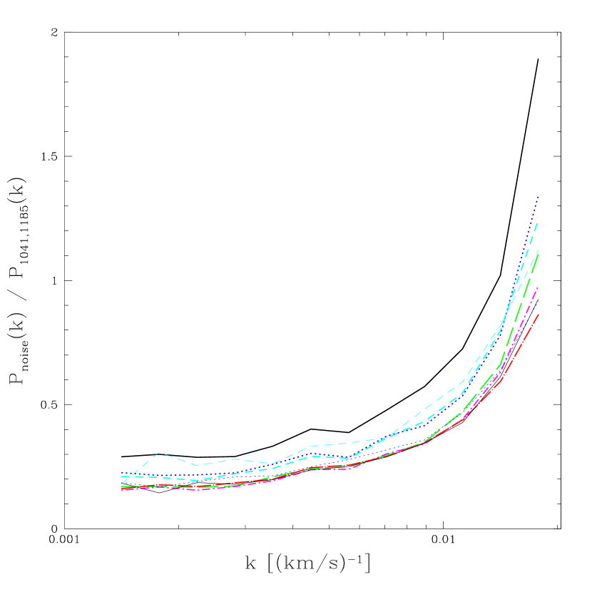
The noise power is significant (20-30%) on all scales, but diverges at high where the resolution suppresses the absorption power. The lowest redshift bin has the most noise, due to the lower Ly forest power combined with extra noise at the short wavelength end of the spectra.
Figure 12 shows our window matrix (at ), which we proceed to diagonalize.
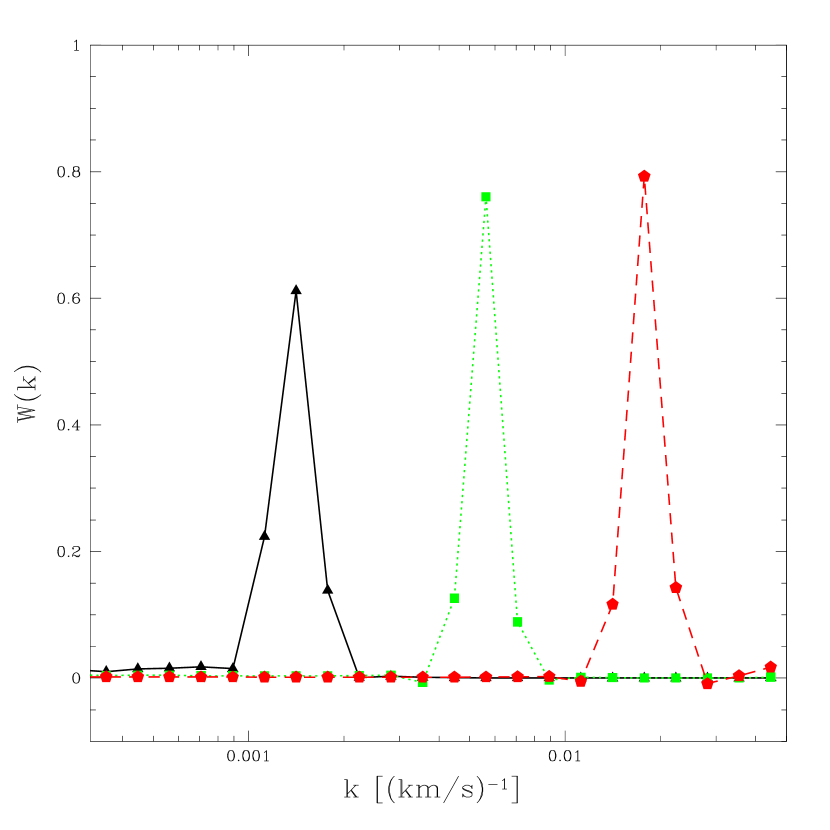
The matrix is reasonably close to diagonal already, with large contributions only from adjacent bins. It is useful to diagonalize the matrix at this stage, rather than waiting until the model-fitting stage, because this allows us to compute bootstrap errors directly for the final bins (the bootstrap error calculation and window matrix diagonalization do not perfectly commute).
Figure 13 shows the ratio of the bootstrap errors to the errors estimated assuming the data are Gaussian.
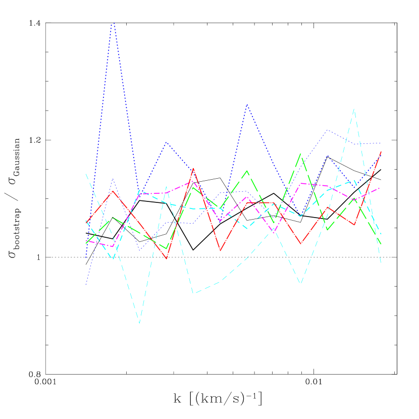
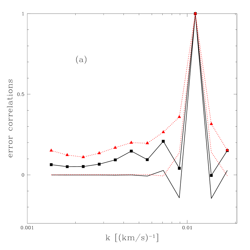
We did not apply the Gaussian floor to the bootstrap errors when making this figure. Typically the bootstrap errors are 0-20% larger than the Gaussian errors. Figure 14 shows examples of the estimated correlation between the errors, at .
![[Uncaptioned image]](/html/astro-ph/0405013/assets/x17.png)
We note that diagonalizing the window matrix noticeably reduces the error correlations. The bootstrap errors are, in contrast to the Gaussian errors, noticeably correlated ( when , where and label the bins) across the full range. These differences between bootstrap and Gaussian errors are not necessarily an indication of intrinsic non-Gaussianity in the absorption fluctuations. Possible alternative explanations for the differences include the uncertainty in the mean flux value that each chunk of spectrum is divided by and the uncertainty in the noise-subtraction term for each chunk, neither of which are included in the Gaussian estimate and both of which would increase the error in a way that is correlated across bins.
3.4 Background Subtraction
Our background subtraction is the power in the wavelength range Å. Figure 15 shows and for comparison.
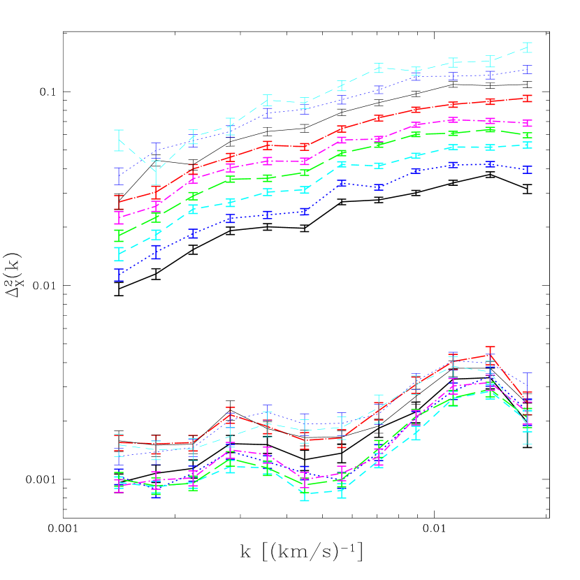
The bump at in is probably due to the CIV doublet at separation . The bump at may be due to the SiIV doublet at separation . Figure 16 shows .
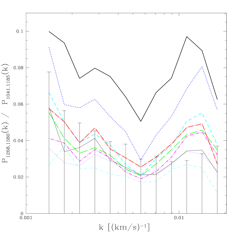
We see that, even though the background power is a small fraction of the Ly forest power, it is quite significant when compared to the small size of the errors on the Ly forest power. It is important to remember that even a small overall systematic error can be very significant if it covers many data points (e.g., a error over 100 points shifts the mean by ).
We are going to subtract the power in the range 1268-1380 Å from the Ly forest power, but it is informative to measure the power at other places in the quasar rest frame for comparison. The range 1409-1523 Å includes CIV absorption (at 1548.2 and 1550.78 Å) but excludes SiIV (at 1393.75 and 1402.77 Å) and shorter wavelength transitions. Figure 17 shows .
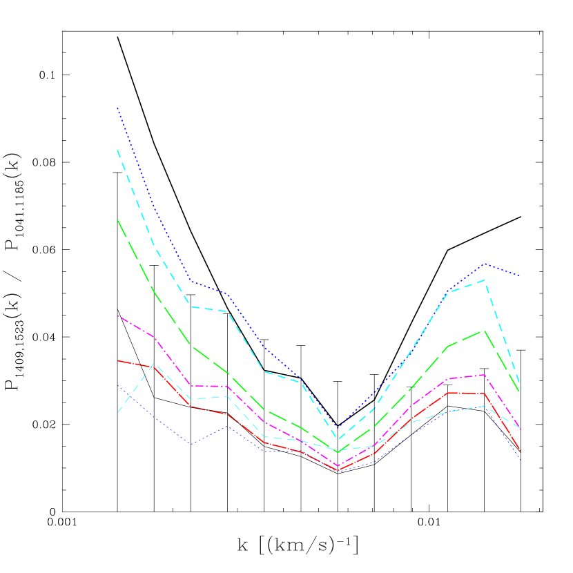
If all of the power was coming from metal line absorption, the power in the range Å should always be less than the power in the range Å. As we see in Figure 18, which shows the difference in the background fractions, , the power in is greater than except on large scales.
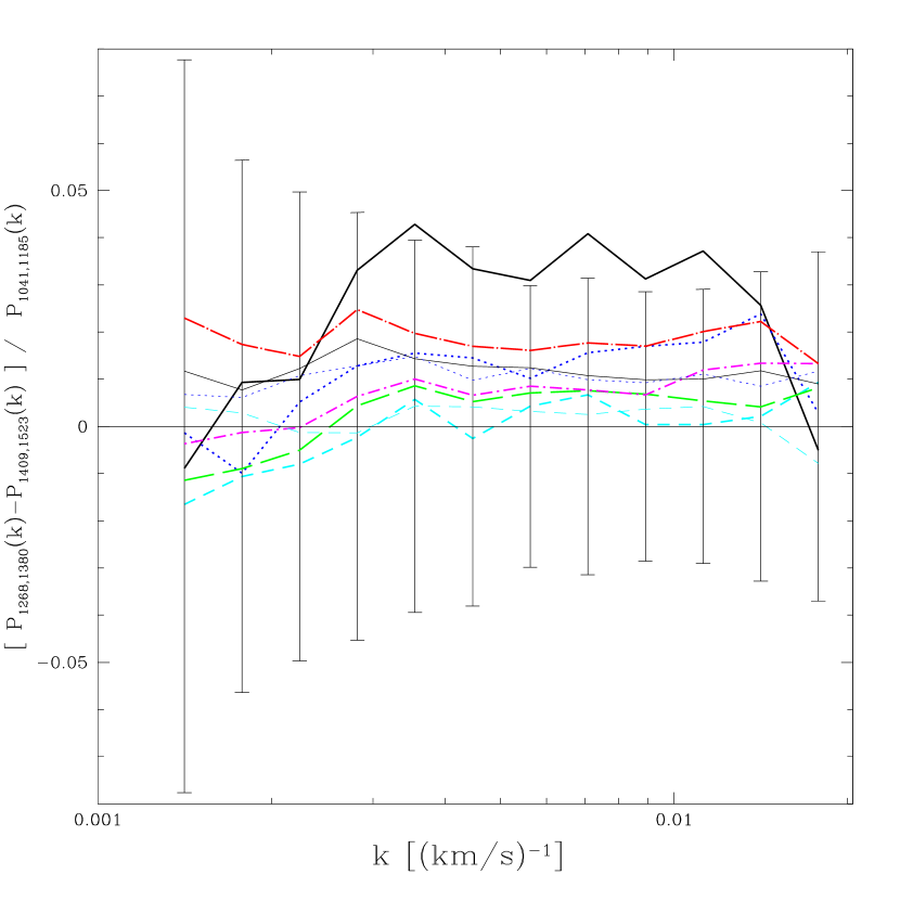
The difference on large scales suggests that there is tiny amount of power left in the quasar continua (in spite of our division by the mean continuum), which is larger in the range 1409-1523 Å than in the range 1268-1380 Å. Finally, Figure 19 shows , past the wavelength of CIV absorption.
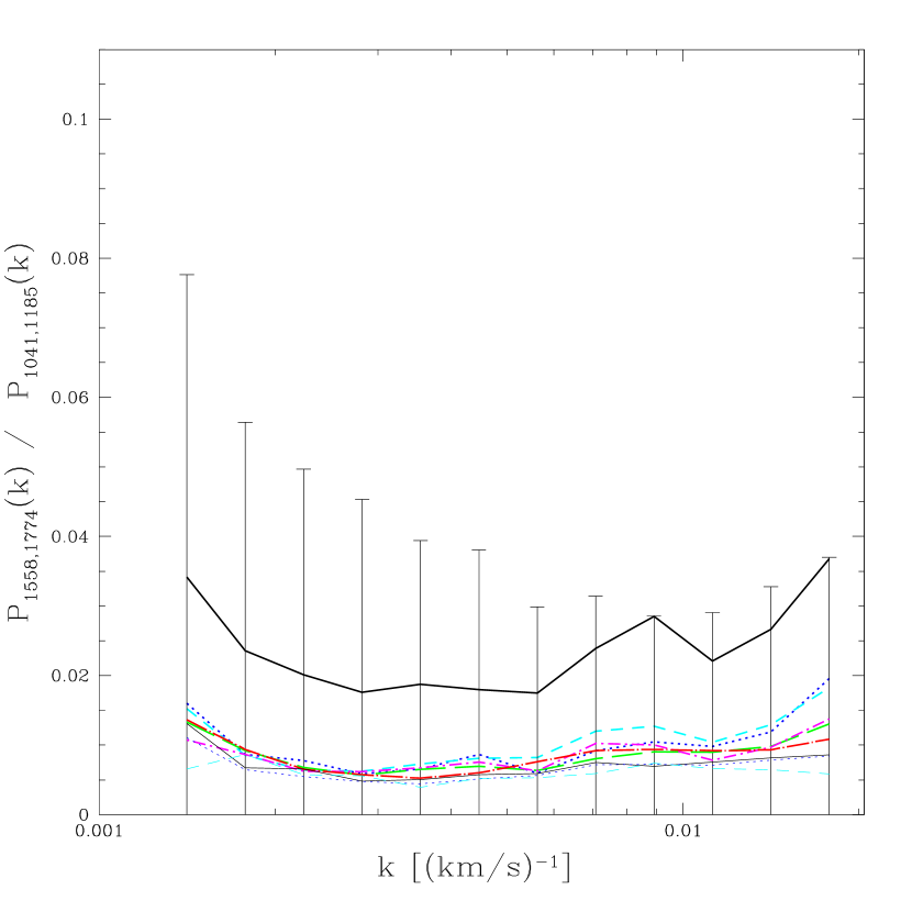
The reduction of power relative to shorter wavelengths is dramatic, but not surprising since CIV is the most common metal absorber. It does suggest however that most of the power is due to metals and not continuum fluctuations, unless the continuum in the range 1558-1774 Å has significantly less power relative to other intervals studied here (which is admittedly not inconceivable). It seems likely, although we are not certain, that the background power has a noticeable contribution from measurement-related problems, because the alternative is a very sudden increase in metal absorption power.
What is the upshot from these studies? The metal absorption appears to contribute a small but significant amount of power, which should also appear in the Ly forest region. We subtract this power from the power measured in the forest. There is some indication of measurement-related problems in our lowest redshift bin. The power contributed by deviations of the quasar continua from their mean appears to be small.
While the idea that contains almost exclusively power due to simple metal absorption seems plausible at this point, when we perform consistency checks in §4.4 we find evidence that this is not the case. Splitting the data set used to measure in half based on the noise level in each spectrum, we find that the power in the halves is significantly different, by as much as 50% in some bins. Splits based on several other properties of the data (e.g., sky to quasar flux ratio) also show significant differences, but we find that these differences can all be accounted for by the difference in the basic noise level in the subsamples. Splits of the Ly forest data set show similar trends in with the splitting parameters, although the fractional differences are much smaller. While we don’t know the source of this noise dependence, it is not hard to imagine relatively benign reasons for it. For example, if sky subtraction is imperfect this would add an increasing amount of power as the sky flux, and thus noise level, increases relative to the quasar flux. The procedure we describe next would remove this power.
Since we know that depends on noise it seems logical to subtract the value of corresponding to the level of noise in the forest, rather than the best measured value of , which is dominated in practice by data with less noise. If we had simply misestimated the noise by an overall factor, for example, the errors in and would cancel for this form of subtraction. To implement this idea, we model the background subtraction term as a linear function of the noise level,
| (13) |
where is the mean noise level in the data computed in the same way as the mean flux level (this is the mean of the normalized noise, i.e., after division by continuum and mean flux). The choice of a linear relation is arbitrary but it does the job (see §4.4) better than the alternatives we tried. We compute and for each value of and using a linear fit to the full sample of spectra that probe , weighted by the Gaussian estimate of the error on each point for each spectrum. When the time comes to subtract the background from to obtain , we use computed in the Å wavelength range to compute the appropriate subtraction term. Figure 20 shows the extra power subtracted through Equation (13), beyond what we would subtract if we simply used from Figure 16.
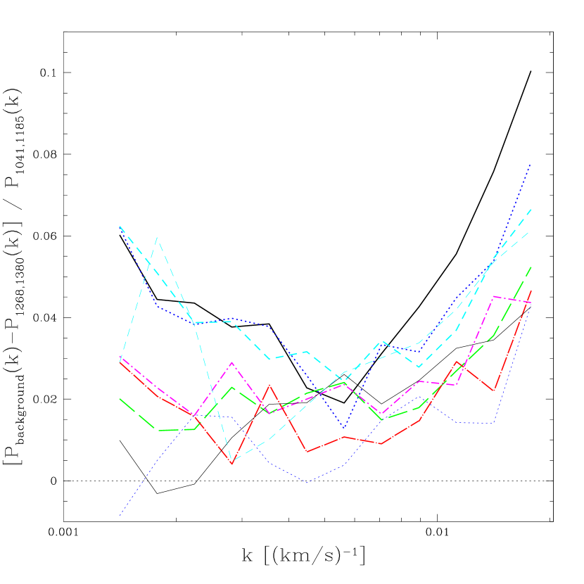
It is typically less than 4% of the Ly forest power, but rises to 10% at the highest for the lowest redshift.
The reader who is paying attention may complain that we have no compelling reason to believe that this source of noise-dependent power that we do not understand depends on noise in the same way inside and outside the Ly forest region. This would be true, except that when we follow this prescription for background subtraction the differences in between subsamples are removed (see §4.4). This would be a remarkable coincidence if our model for the subtraction was not substantially correct.
Note that the background power has much smaller (absolute) statistical errors than , mostly because there is simply less power, but also because there are more quasars probing a given redshift interval.
4 Consistency Checks
In §4.1 we describe how we use fits of theoretical models to the results to help understand the importance of any systematic errors. We plot the correlation function of the Ly forest in §4.2 and use it to identify a significant contribution to from SiIII absorption. In §4.3 we examine the effects of modifications of our procedure. In §4.4 we break the data set up in many different ways to look for dependencies of that should not exist. In §4.5 we discuss the possibility that continuum fluctuations contribute significant power. Finally, we compare our results to past measurements in §4.6.
4.1 Rudimentary Fitting of Theoretical Models
The ultimate purpose of measuring the Ly forest power spectrum is to determine cosmological parameters by comparing the observed to the predictions for different cosmological models. For the CDM models supported by present observations, the universe is nearly Einstein-de Sitter at , so cosmology influences the Ly forest almost entirely through the linear theory power spectrum of the mass fluctuations, , at and (roughly 1 comoving h/Mpc, depending somewhat on the model). We usually parameterize by its amplitude, , slope , and curvature , where we use and as the pivot points.
A full discussion of the details of theoretical modeling of using numerical simulations is beyond the scope of this paper. Furthermore, the theory of the Ly forest is perhaps less certain than the observations, so we want to present the observational results un-tarnished by theoretical interpretation. However, it is very useful to interpret the possible systematic errors in the appropriate context of cosmological model fitting. In other words: without model fitting, it is difficult to know how important a given change in is.
In this paper we take a cautious approach to the theoretical model fitting – we perform fits to different estimates of computed using modifications of the extraction procedure or different subsamples of the data, however, we do not give the central result, only the deviations in the results from the value obtained from our preferred . These deviations in fitting results should give the reader a useful indication of the importance of systematic effects in the data, regardless of the reader’s opinion of the theory.
The simulations and fitting procedure that we use are described in McDonald et al. (2004), where we present the final result. We use a CDM transfer function, and perform the fit with and as free parameters (because is not tightly constrained by the present Ly forest data alone, we fix the primordial running , not to be confused with , to zero). Unless otherwise specified, we perform the fits using the 108 points in the ranges and . We allow for some error in our noise estimate by permitting the noise subtraction terms to vary independently in each redshift bin by 5% (9 extra free parameters to fit for, constrained by Gaussian likelihood function with this rms width). We also allow a single overall parameter describing the squared resolution error to vary with rms constraint .
The Ly forest model in the simulations is controlled by the externally constrained functions , the mean absorption, , the temperature at overdensity 1.4, , the logarithmic slope of the temperature-density relation, and a reionization parameter that we will call . is described in our fits by the 10 parameter formula , where labels our 9 redshift bins, gives the arbitrarily normalized dependence and is an overall normalization. We have performed a preliminary analysis using the formalism in §2.5 to measure from SDSS data and we use this to constrain the parameters (the error on each redshift bin is ). Because the SDSS analysis does not constrain the overall normalization, we leave free except for the additional constraint that we require interpolated to to match the HIRES constraints (see McDonald et al. (2000) – we have modified the numbers slightly and increased the errors to allow for systematic uncertainties, as discussed in Seljak et al. (2003)). We parameterize and by quadratic functions of (3 parameters each) with the external constraints K and at (see McDonald et al. (2001) – we added 2000 K in quadrature to the temperature errors to allow for systematic errors). Note that there are other, sometimes more precise, measurements of (Schaye et al., 2003; Bernardi et al., 2003) and the temperature-density relation (Schaye et al., 2000; Ricotti et al., 2000) in the literature – our choice of McDonald et al. (2000) and McDonald et al. (2001) for this example is simply for convenience. The redshift of reionization and post-ionization temperature of the gas influence Ly forest predictions because the smoothing of the gas on small scales depends on its pressure history. At the level of precision we care about, this dependence can be captured by a single parameter. In our modeling, we use to interpolate between two reasonable boundaries, reionization heating of the gas to 25,000 K at or to 50,000 K at , both of which are consistent with our temperature constraints . However, in this paper we fix , because it is weakly constrained by the data and the hard lower limit we have to impose on the redshift of reionization leads to non-Gaussian errors on the power spectrum parameters we are interested in (this is a problem of presentation, not of principle).
Figure 21 shows our first fit to the standard results.
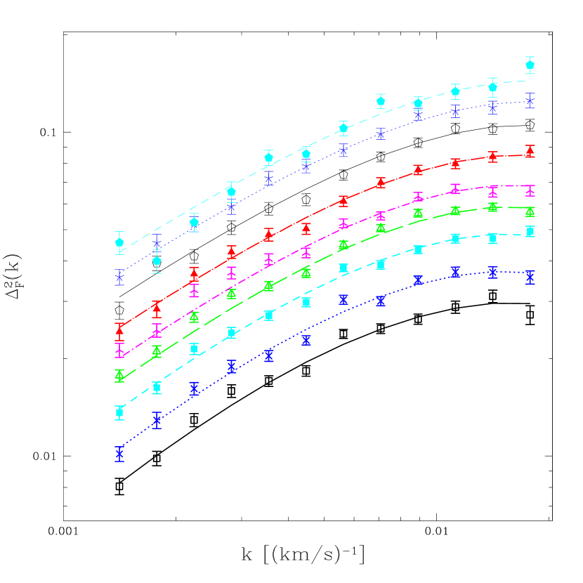
The value of is much too high for approximately 106 degrees of freedom (we are marginalizing over a large number of nuisance parameters, but these generally are externally constrained so they do not reduce the number of degrees of freedom). Including as a free parameter does not improve the fit significantly. It appears that much of the disagreement comes from bumps in the power spectrum, e.g., at . This motivates us to look at the correlation function of the flux.
4.2 The Correlation Function and the SiIII Cross-Correlation
Sometimes features in the power spectrum are easier to understand by looking at the correlation function, ( is as usual a stand-in for wavelength differences, as is in this case). We show the normalized correlation function, for the first six redshift bins in Figure 22.
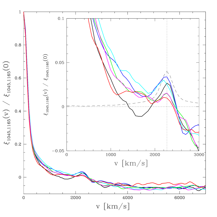
The correlation function shows the expected behavior – positive for small , negative for large – except for an obvious bump at . We focus on this bump in the inset panel of Figure 22. The most likely explanation seems to be cross-correlation between Ly and SiIII absorption. SiIII absorbs at Å, so the SiIII absorption by gas at some point along the line of sight will appear in the spectrum separated by 2271 km/s from the Ly absorption by the same gas. We see that the bump in appears at this separation, and note that the features that ruined our power spectrum fit appear at the expected multiples of . Note that this is the only correlation seen; another metal correlation one might expect to see is NV (Å), but there is no apparent feature at the corresponding velocity differences (km/s), as seen in figure 22.
What should we do about this SiIII-Ly cross-correlation, since the poor suggests that it is too significant to ignore? Our first guess might be that the SiIII-Ly correlation is a simple offset version of the Ly-Ly correlation, i.e., something like . The simplest way to model this is to assume that the SiIII structure is equal to that of the Ly forest up to an overall normalization, , where is for Ly only and . The corresponding correlation function is
| (14) |
with corresponding power spectrum
| (15) |
where unsubscripted and are understood to mean Ly-Ly. For our first fit to accounting for SiIII using equation (15), we assume , with as a single extra free parameter of the fit. We find a remarkable improvement in , from 193.7 to 130.9. We find (, depending on the redshift). The small value suggests that the relative contribution of SiIII to the autocorrelation is , which will not affect our fit results significantly (see §4.3). We thus only need to estimate the cross-correlation term. We also tried allowing a power law dependence for , but the improvement in fit, , was not significant.
In the inset panel of Figure 22 we plot scaled , to show how the shape of the bump compares to the zero-lag correlation. It is difficult to compare the shapes by eye, because of the slope of the underlying correlation, but it appears that this model explains the cross-correlation reasonably well. We can allow for a change in scale using the slightly more general form
| (16) |
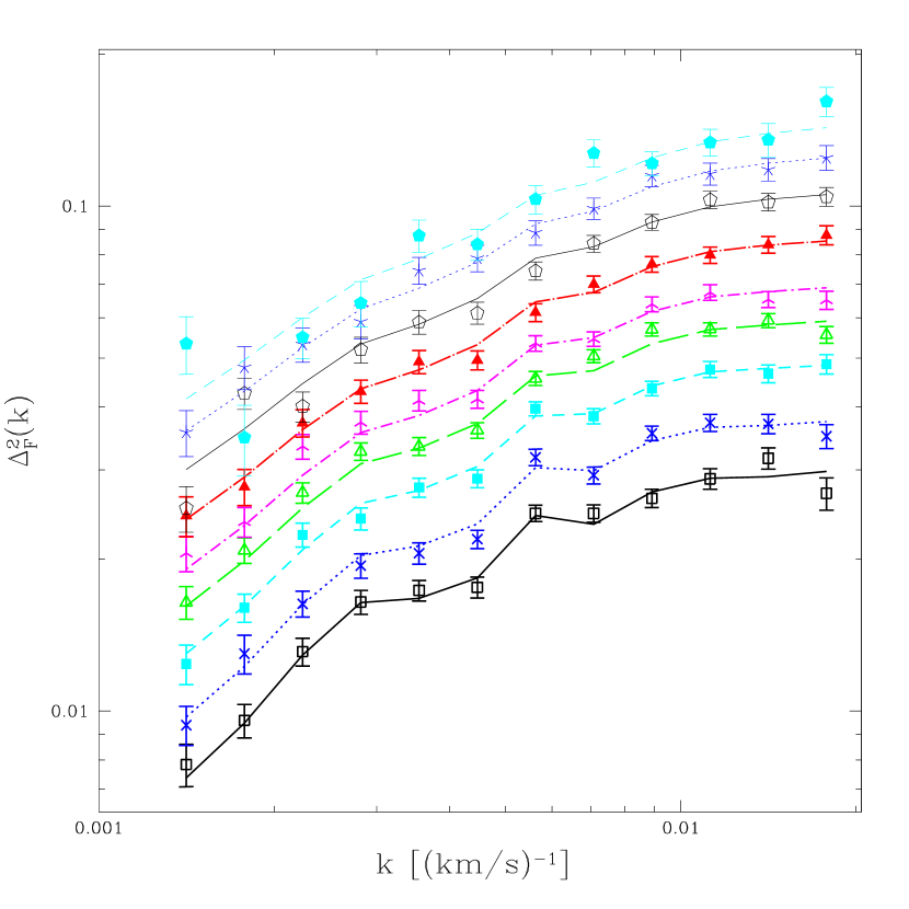
Allowing to vary freely only improves by 0.7 (note that the logarithmic -binning that we use may reduce our ability to constrain these parameters). The error bars on other parameters may increase when we include dependence of and allow to be free, so to be conservative one probably wants to leave them free even though they are not needed. In our standard fit in this paper, we allow to have dependence but fix . We show the improved fit to in Figure 23.
4.3 Modifications of the Procedure
The pipeline developed for this analysis includes many improvements and corrections that were added throughout the development. It is worth taking a step back to ask how important the various corrections are for the final result. Table 1 lists various modifications of our procedure (described individually below), and quantifies their effects on the fit results. In each case we show the change in the best fit and relative to our standard fit, and their error bars for comparison to the standard fit. We give to indicate the goodness of fit of the theory to the modified measured . We reiterate that we are not asserting the correctness of the theory that we use in the fitting – we give these values and other fitting results only to show trends. We list between the standard procedure best fit and the variant best fit, to give an indication of how significant the deviation is (this is necessary because the errors are correlated so simply knowing and and their errors does not give the full picture – see Figure 26 for an example of the full error contours). Because the statistical fluctuations between these different fits should be small, a difference (or even less) should be interpreted as “significant”, however, since we believe that our standard fit is better or more conservative than all of the variants, our systematic error should generally be smaller than the deviation shown. Note that where applicable the changes in procedure are only applied to the calculation, not the result that is used in the background subtraction (small changes in have no effect on the final results).
Our first variant is to not diagonalize the window matrix. Figure 24 shows the measured power spectrum before and after diagonalization.

Figure 25 shows the ratio of the diagonal errors after diagonalization of the window matrix to before diagonalization.
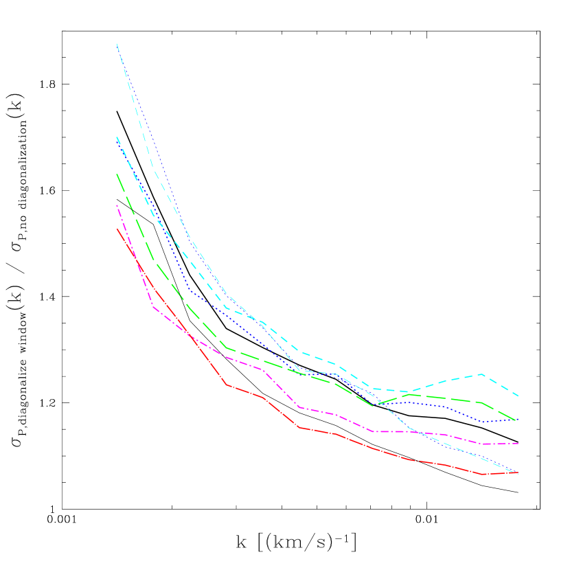
Not diagonalizing the window matrix does lead to a significant change in the fitted parameter values, and the error on decreases by about 12%. We are, in effect, using information from a wider range of scales, but this forces us to use theory results outside their range of validity (e.g., at low we need to extrapolate beyond the size of our simulation boxes). Note that the change in error on , from 0.024 to 0.021 implies that we should expect a random difference between the two results with typical size , i.e., what might seem like a surprisingly large part of the difference between the results could be random.
As discussed above, the correction for SiIII-Ly correlation is very important to the goodness of our fit. It is less important for the best fit values, changing them only by for and for . Normally we allow a power law dependence on redshift for the amplitude of the SiIII-Ly correlation, but removing this freedom makes almost no difference. Allowing the correlation scale for the SiIII-Ly correlation to be different than for Ly-Ly (freeing in eqn. 16 – we usually fix this in this paper for technical reasons) has only a very small effect. Including the SiIII-SiIII autocorrelation term (the part of eqn. 15) in the fit has essentially no effect.
For our standard fit, we allow variation in the noise amplitude at each redshift, represented by a multiplicative parameter subject to a 5% rms Gaussian constraint. Our fitting procedure then marginalizes over this component. Reducing this constraint to 0.5% (i.e., fixing the noise) produces no change in our fit result, and does not even reduce the error bars noticeably. Leaving the noise essentially free makes a noticeable difference in the fit results, decreasing the amplitude by about , increasing its error by 20%, and decreasing to 123.8. Changes at this level are expected when we remove the constraints on some parameters, and do not imply that the constraints were too small (i.e., we are effectively removing 9 data points from the fit so we generally expect a decrease in , increase in the error bars, and some corresponding drift in the parameter values). Removing our spectrum-by-spectrum noise estimation makes very little difference. Finally, we note that if we did not correct the noise as discussed in §2.3, the results would change significantly. As an example, we show the fit results in the plane in Figure 26, for our standard case and these noise-related variants.
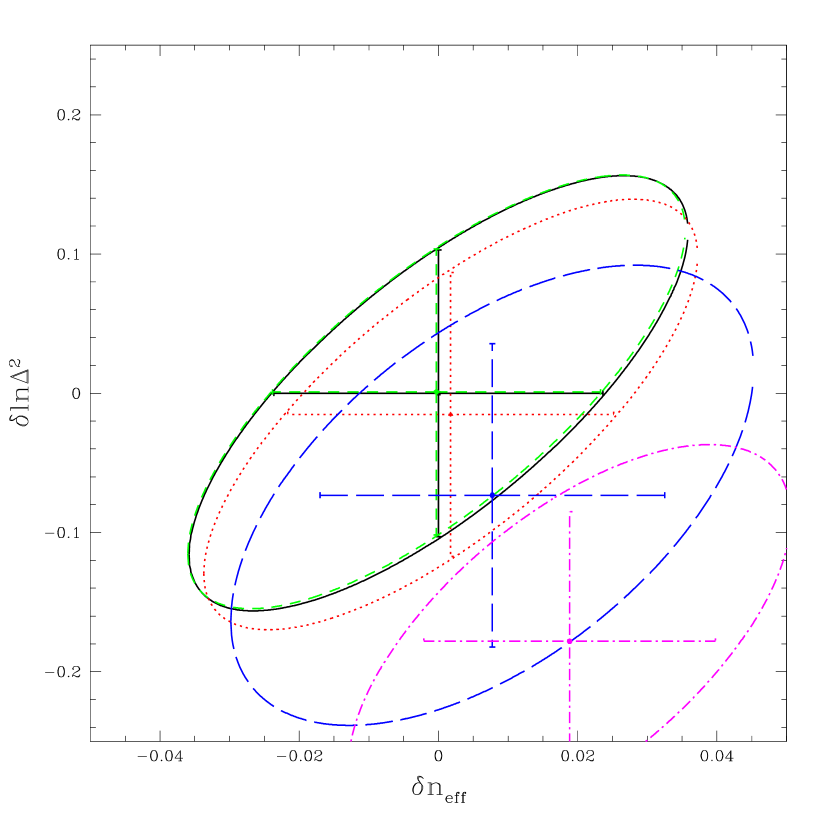
We show the ratio of the power without individual noise estimates for each quasar to our standard case in Figure 27.
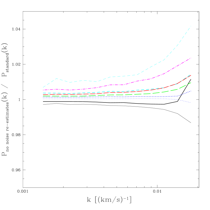
Our requirement that the principal components of the error matrix have at least the Gaussian level of variance makes no difference to the fit results, although it improves for the fit a little bit. Simply using the Gaussian error matrix instead of bootstrap errors makes no difference to the fit results but increases significantly. Ignoring the bootstrap error correlations increases the error on by about 12%, and significantly reduces .
We normally use the range Å for our background subtraction (i.e., subtract ). Removing the background subtraction entirely reduces the inferred amplitude by , and the slope by , and results in a very large (the error on also decreases significantly, but this is mostly because of the change in the best fit values, not because of uncertainty in the background subtraction). (Note that removing the background subtraction, which increases , decreases the inferred amplitude because the fitted decreases more than enough to offset the increase in .) Clearly the background cannot be ignored. Using instead produces a somewhat disturbingly large 0.028 () increase in . We expect the longer wavelength range to give a less accurate estimate of the background power, because some metals are missing, but further investigation shows that most of this difference is probably caused by CIV BALs adding power to the Å region. As we see in Table 1, removing the adjustment for noise dependence of the background (see Equation 13) brings the two background regions closer together (this is reflected in Figure 18). Adding the 147 BAL quasars identified by our automated algorithm leads to a huge discrepancy (0.094 in ) when we use the background, but only when we adjust for noise level (without this the discrepancy for , not shown in the table, is only 0.029). Note that the BAL cut makes essentially no difference to our standard fit using the background. All of these differences are easy to understand: First, BALs are known to be strongest in CIV absorption (Hall et al. (2002)), so it is not surprising that we see the effects of BALs primarily in this wavelength region. Second, both our original by-eye and subsequent automated removal of BALs inevitably identify the features more easily in less noisy data, so the power from BALs naturally shows up when we intentionally use the noisier spectra for the background power. The fact that removing the 147 most obvious BALs has essentially no effect on our basic result gives us confidence that any remaining BAL features in the Ly forest and Å regions are not significant.
To investigate the effect of a systematic uncertainty in the spectral resolution, we include in our fits an overall factor of the form multiplying the power spectrum, where is a free parameter. In our standard fit we impose an external constraint on , rms. Essentially removing this freedom has no effect on the fit, while leaving essentially free increases the error on the amplitude by 40%, and increases by (the change in fitted amplitude is certainly consistent with drift from the increased error). As we show in Figure 5, our standard fit should be conservative.
Simply dividing each chunk of spectrum by its mean instead of also dividing by the mean continuum before estimating the power from the chunk makes little difference to the fit results. Division by the mean continuum actually increases the measured flux power by %, as we show in Fig. 28.
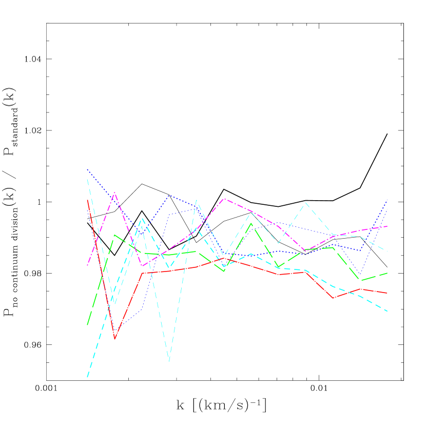
We have performed a preliminary PCA analysis to try to model fluctuations around the mean continuum. When we use continua for each quasar composed of 13 PCA eigenvectors, our results change only a little ( is reduced by ), and increases, probably an indication of the unsatisfactory level of noise that we know remains in our estimates. As we see in Figure 29, the modification of adding a large constant to the weight matrix to make our measurement less sensitive to the mean of each chunk has little effect (the effect is larger on larger scales).
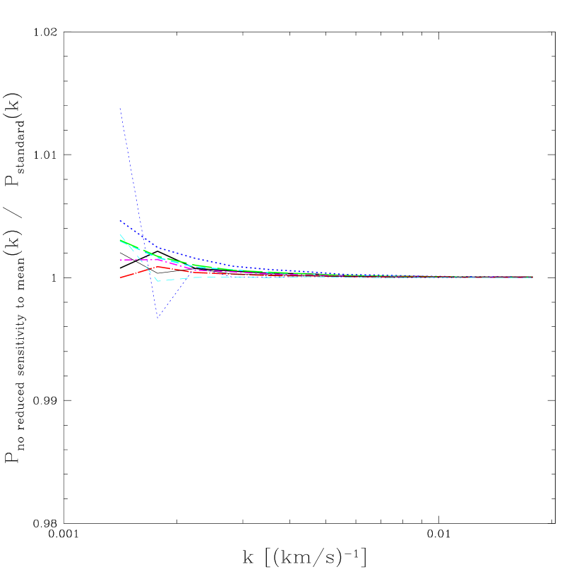
The line “no bin-redshift correction” in Table 1 refers to removing the correction for evolution in the power across the width of the redshift bins (see eqn. 8). We see (Fig. 30) that this correction mostly affects the lowest redshift bin (where the low- edge of the bin is empty of data) and has little effect on the fit (not surprisingly, leaving out this correction increases ).
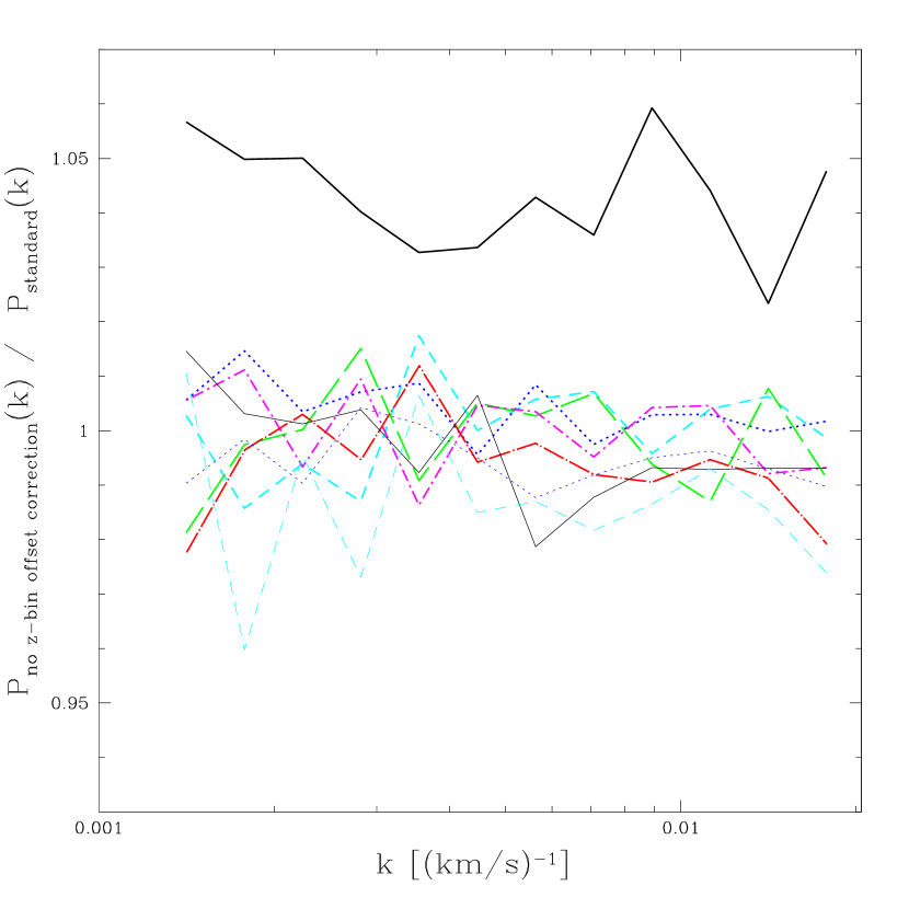
The line “ignore correlation” in Table 1 shows the change in the fitted parameters if we naively use the given noise estimates for weighting without accounting for the fact that there is a correlation between the flux estimate and the noise amplitude estimate for each pixel. Figure 31 shows that the bias is a fairly constant 3-5% increase in the flux power.
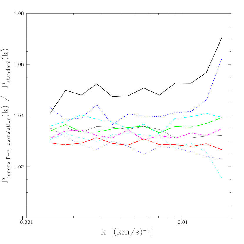
The difference is not actually caused by the change in weighting used in the power spectrum estimation – instead, the power is biased high because the estimation of the mean that each chunk of spectrum is divided by is biased low because low-flux pixels have smaller noise estimates. Ignoring this effect does not change our fit results. Normally we base our estimation of the amount of the noise that is due to quasar flux on the separate estimates we have from the spectral reduction pipeline for the flux, sky, and read-noise contributions, however these estimates do not add up to the total noise reported by the pipeline. If we rescale the individual numbers to make them consistent with the total (not necessarily the correct thing to do) we see that the fit results are not changed significantly (the line “rescale ” – we use to refer to noise computed using the separate flux, sky, and read-noise estimates), although the power does change by as much as 3% (Fig. 32 – this difference would be a bit larger if we did not directly measure and correct for the cross-correlation between the noise amplitude and flux).
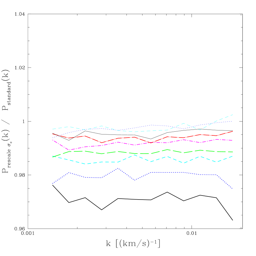
Finally, our power spectrum extraction code has a bias (partially related to division by the mean of each chunk of spectrum), that we correct for by dividing the result by Equation 11. Removing this correction decreases the estimated by about and increases the amplitude by a similar amount. The combined change is actually quite significant because it is transverse to the degeneracy direction for these parameters.
To summarize, most of the effects described above are small relative to the statistical errors on the final estimated parameters. We understand the cases where the difference is significant, and expect that our standard method will be much more accurate than the difference between it and the variants (we show these variants to help the reader better understand our measurement). These tests give us confidence that the final results are very robust to small changes in the analysis pipeline.
How sensitive are these conclusions to our assumptions about the nuisance parameters, , , and , i.e., if these constraints improve in the future, will we need to worry more about systematic errors in ? We investigate this by first fixing all the parameters in the fit (including removing the noise amplitude uncertainty, resolution uncertainty, and freedom in the SiIII correction), so the only uncertainty is on . Table 1 (the “fixed nuisance parameters” line) shows that the error on the amplitude improves dramatically, by a factor of 5. The error on improves by a factor of 2. So in principle the amplitude error can be improved a lot relative to potential systematic errors, and improved as well (see also Mandelbaum et al., 2003). The next line (“optimistic ”), where we assume the HIRES constraint on is improved by a factor of 5, and the SDSS constraint by a factor of 2, shows that is substantially degenerate with (as expected), but is less degenerate. Improving the constraints on and by factors of 5, in addition to the improved constraints on , leads to little further improvement. Finally, for comparison, we tried simply reducing the errors on by a factor of , and found that the error on decreases by almost the same factor (1.6), but the error on decreases less (a factor of 1.2). SDSS will collect a factor of more data than we have in the present sample. We conclude that the error on can easily be reduced by simply gathering more data, while improvements on can be made by improving the errors on .
| VariantaaThe meaning of each variant is explained in §4.3. | bb of the fitted parameters relative to the standard parameters, using the errors from the variant fit. | cc for the fit (essentially unrelated to ). | ||||
|---|---|---|---|---|---|---|
| Standard fit | 0 | 0.10 | 0 | 0.024 | 0 | 129.7 |
| No window diagonalization | -0.06 | 0.10 | -0.024 | 0.021 | 1.4 | 129.5 |
| No SiIII correction | 0.04 | 0.10 | 0.017 | 0.021 | 0.7 | 193.7 |
| -independent SiIII | 0.00 | 0.10 | 0.0 | 0.024 | 0.0 | 130.9 |
| variable width SiIII | -0.02 | 0.11 | -0.006 | 0.025 | 0.1 | 129.0 |
| Include SiIII-SiIII term | -0.02 | 0.10 | -0.003 | 0.023 | 0.0 | 132.1 |
| % | 0.00 | 0.10 | -0.000 | 0.024 | 0.0 | 130.3 |
| % | -0.08 | 0.12 | 0.008 | 0.025 | 1.1 | 123.8 |
| No individual noise re-estimation | -0.02 | 0.10 | 0.002 | 0.023 | 0.1 | 128.1 |
| Believe pipeline noise | -0.20 | 0.11 | 0.019 | 0.021 | 9.6 | 129.9 |
| No Gaussian floor on errors | 0.01 | 0.10 | 0.002 | 0.024 | 0.0 | 133.1 |
| Gaussian errors | 0.02 | 0.10 | 0.001 | 0.023 | 0.1 | 151.7 |
| Ignore error correlations | 0.04 | 0.11 | 0.002 | 0.027 | 0.2 | 117.2 |
| No background subtraction | -0.20 | 0.10 | -0.022 | 0.019 | 3.6 | 169.6 |
| Background 1409-1523Å | 0.05 | 0.10 | 0.028 | 0.025 | 1.5 | 133.2 |
| No background noise matching | -0.07 | 0.10 | -0.004 | 0.021 | 0.7 | 142.3 |
| Previous, but use 1409-1523Å | -0.06 | 0.10 | 0.008 | 0.022 | 1.7 | 143.1 |
| No automated BAL cut | 0.01 | 0.10 | 0.003 | 0.023 | 0.0 | 127.0 |
| Previous, but use 1409-1523Å | 0.14 | 0.10 | 0.094 | 0.025 | 16.0 | 156.6 |
| resolution error | -0.11 | 0.14 | 0.015 | 0.024 | 1.4 | 126.4 |
| resolution error | 0.02 | 0.10 | -0.003 | 0.024 | 0.3 | 130.4 |
| No continuum division | 0.02 | 0.10 | 0.002 | 0.024 | 0.1 | 132.2 |
| PCA continuum division | 0.02 | 0.10 | -0.010 | 0.024 | 0.8 | 139.1 |
| No reduced sensitivity to mean | -0.00 | 0.10 | -0.002 | 0.024 | 0.0 | 130.5 |
| No bin-redshift correction | -0.02 | 0.10 | -0.006 | 0.023 | 0.1 | 137.2 |
| Ignore correlation | 0.00 | 0.10 | 0.002 | 0.024 | 0.0 | 128.7 |
| rescale | 0.00 | 0.10 | 0.002 | 0.024 | 0.0 | 129.0 |
| No code bias correction | 0.06 | 0.10 | -0.013 | 0.024 | 3.0 | 132.3 |
| 8000 bootstrap sets | 0.00 | 0.10 | 0.000 | 0.024 | 0.0 | 128.5 |
| fixed nuisance parameters | 0.083 | 0.021 | -0.025 | 0.012 | — | — |
| optimistic | 0.068 | 0.062 | 0.009 | 0.019 | — | — |
| optimistic , | 0.002 | 0.082 | -0.014 | 0.021 | — | — |
| optimistic , , | 0.002 | 0.051 | -0.016 | 0.018 | — | — |
| errors divided by | -0.051 | 0.081 | -0.000 | 0.015 | — | — |
Note. — , .
4.4 Subsamples of the Data
Another way to test for systematic errors is to search for internal discrepancies between the different subsamples of the same data. Of course, there are only a finite number of possible subsamples we can try, so this test cannot be fully exhaustive. In addition, with many such tests performed one must worry that some will give an apparently statistically significant deviation just by random chance. Table 2 shows results of splitting the data into roughly equal weight subsamples, defined by various properties of the spectra that, at least at first glance, should not be correlated with the measured power. In practice, we rank the spectra by the property of interest and split the sample into halves by requiring that the Gaussian errors on the point are equal for the two halves (the bootstrap errors will not be precisely equal). We list the probability of obtaining greater than the value computed by differencing the power spectra (these differences include the different background subtraction computed using eqn. 13 for different noise levels). We also list the fitting parameter results for each subsample, and give the probability for obtaining the observed level of difference between the fits. Because these subsamples are basically independent, deviations within the error bars are expected and are not an indication of systematic errors. We describe these subsample splits below.
| Split | aaProbabilities may not be fully reliable because we have not demonstrated that is properly distributed. | bbThe subsample fit results cannot be combined to produce the result of the fit to the full data set because the underlying nuisance parameters were not required to be the same. | ||||
|---|---|---|---|---|---|---|
| (points) | (fit) | |||||
| 40% | 51% | |||||
| noise | 10% | 76% | ||||
| noise (raw)ccThe “noise (raw)” line shows the comparison without accounting for the noise dependence of the background. | 0.0006% | 61% | ||||
| sky | 5.9% | 93% | ||||
| 34% | 49% | |||||
| read noise | 94% | 68% | ||||
| cont. | 33% | 40% | ||||
| resolution | 73% | 32% | ||||
| flexure | 14% | 19% | ||||
| alignment | 29% | 29% | ||||
| exp. | 65% | 63% | ||||
| error on mean | 56% | 67% | ||||
| error on | 40% | 68% |
The power we measure should be independent of the rest frame region of the quasar continuum in which it is measured. Figure 33 shows and to test this expectation.
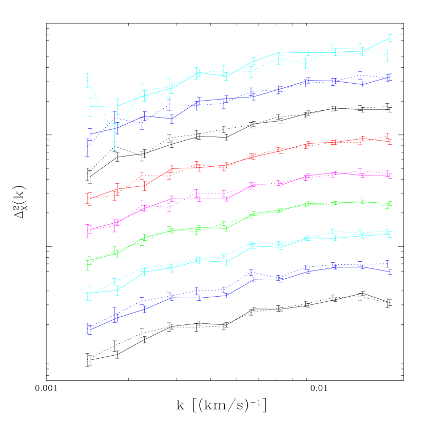
The results look pretty similar, but to compare them quantitatively, we compute , finding for 108 points. The agreement appears perfect. To compare the two in a different way, we perform separate fits of the linear mass power spectrum parameters and to computed from and . The results, given in the first line of Table 2, are consistent within the expected errors. This test provides some evidence that power from continuum fluctuations is not an important contribution to the total, beyond what we would expect from looking at the red side of the Ly emission line. It is possible that the two halves of the forest could have significant extra continuum power, but if they do it has to be the same in each half.
We compute the weighted mean of the rms noise for each chunk of spectrum as we use it to estimate the power spectrum. A split based simply on this noise level, illustrated in Figure 34, produces a small but unambiguously significant discrepancy in the raw measurement of , , though the fit parameters agree within their errors (Table 2, line 3).
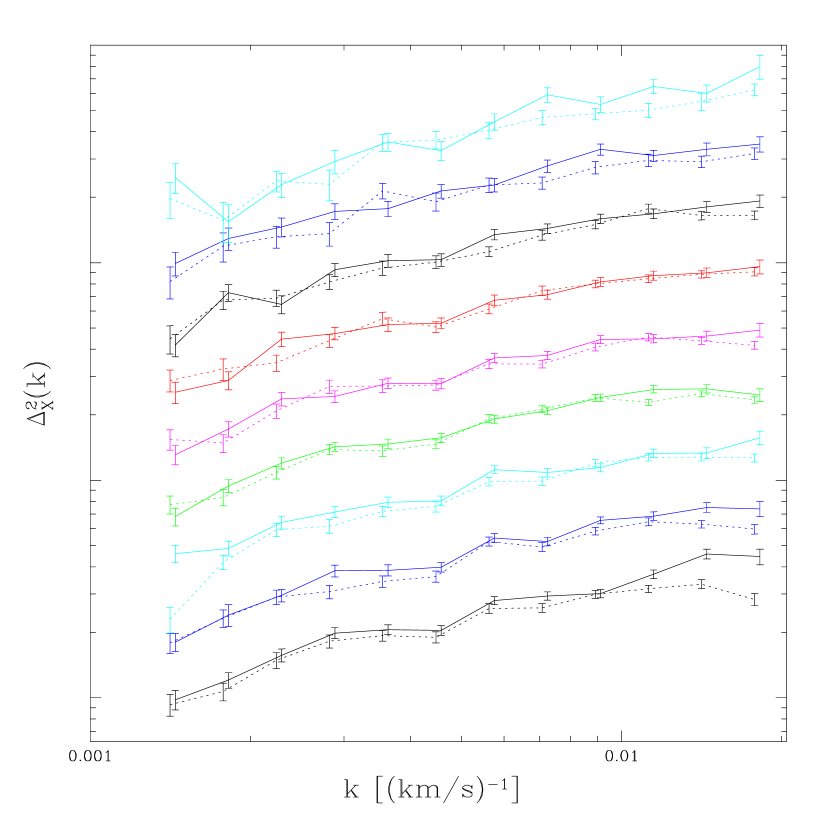
This discrepancy in power is the motivation for, and is largely removed by, our noise-dependent background subtraction procedure defined by equation (13). Figure 35 shows the power that is used for background subtraction, again subsampled by noise level.
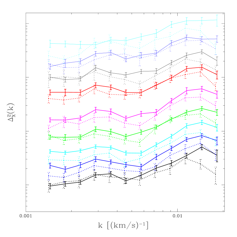
There is a clear difference in power, which is not isolated to a few wavenumbers or redshifts. Once the power is subtracted according to equation (13), we obtain estimates and corresponding fit parameters from the high and low noise subsamples that agree within the errors (Table 2, line 2). Since the fit parameters agree even without noise-dependent background subtraction, it appears that the discrepancy in raw power does not mimic a change in cosmological parameters, and our ultimate conclusions would therefore not change even if we did not implement it. Nonetheless, the origin of the difference remains somewhat mysterious, since we went to great effort to estimate noise correctly.
Two more splits that yield discrepant but show no sign of trouble after the noise-dependent background subtraction are based on the ratio of the mean sky flux to the mean quasar flux and on , the difference between the pipeline estimate of the noise and the sum of our estimates of the quasar flux, sky flux, and read-noise components of the noise. We are not sure what means, since we do not understand the source of noise misestimation in the standard pipeline. Even without noise dependent background subtraction, the fit results did not differ significantly in either of these cases. They are almost surely symptoms of the same noise-related problem discussed above.
The split based on read-noise in the spectra shows good agreement between the measurements, even without noise dependent background subtraction as does a split based on how well the mean continuum matches the quasar spectrum outside the Ly forest, quantified by computing for the difference between the continuum and spectrum (“cont. ” in Table 2). Several other splits that show little or no sign of trouble are based on: the mean value of computed for each pixel when combining exposures (this was the comparison that motivated our spectrum-by-spectrum noise re-estimation), the mean resolution, the movement of the spectrum relative to the detector pixel grid during the observation (“flexure”), the alignment of the pixels in the different exposures for the same spectrum (closely related to flexure), the error on the overall normalization of the spectrum, (see eqn. 2, this error is set by a combination of the noise level outside the forest and the length of spectrum observed outside the forest), and the error on the means computed for the forest chunks (differences at fixed are related to the length of the chunk and the noise in the forest).
Overall, the agreement between our subsamples is excellent, both for the results and the fit results. In some cases this agreement relies on the noise-dependent background subtraction, which we would like to understand better (in no case does the fit agreement rely on this).
4.5 Continuum Power
The power in the mean continuum, for the 4 different rest frame regions identified in Figure 2, is shown in Figures 36a-d, relative to the Ly forest power (the mean continuum power was measured by replacing the quasar flux in each pixel by the mean continuum level at that pixel).
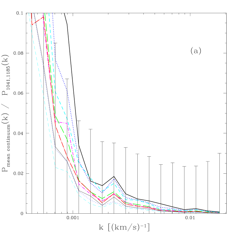
![[Uncaptioned image]](/html/astro-ph/0405013/assets/x40.png)
![[Uncaptioned image]](/html/astro-ph/0405013/assets/x41.png)
![[Uncaptioned image]](/html/astro-ph/0405013/assets/x42.png)
The mean continuum is very well behaved over the range that we use (), but its fluctuations quickly become significant at . What little power the mean continuum shows in our chosen range should be removed when we divide the spectra by the continuum; it is only fluctuations around the mean that matter.
We summarize our strong, but maybe not airtight, argument for believing that continuum fluctuations are not corrupting our measurement as follows:
-
•
The power in the mean continuum is small.
-
•
The results for the measurement in two halves of the forest region, and , agree.
-
•
The power in the background regions, and , agree at the level we care about in the low-noise data, as long as BALs (which mostly affect the latter region) are removed.
-
•
Division by preliminary 13 eigenvector PCA estimates of the continua (i.e., including fluctuations around the mean) does not change the results.
To be quantitatively important despite these arguments, the power in quasar-to-quasar continuum fluctuations in the forest must be substantially larger than the power in the mean continuum itself, the continuum fluctuations in the forest must be substantially different from those in the background regions (despite those regions being similar to each other and the two halves of the forest being similar to each other), and our PCA analysis must be substantially flawed. Further study is warranted, but a big effect seems unlikely.
4.6 Comparison with Past Measurements
There are three measurements already in the literature, McDonald et al. (2000), Croft et al. (2002), and Kim et al. (2004), all using at least some high resolution data. Each uses its own set of redshift bins, so to compare we need a way to interpolate our results to these redshifts. We do this by performing our standard cosmological fit to all of the data (at first – later we will remove some of the past results). This gives us a set of best fit model parameters that can be used to compute the power at any and . Within the range of where we have SDSS measurements, the fit is always dominated by the SDSS points. The fitted curves always match the SDSS results to much better than the size of the errors on the past results, meaning that, for the the purpose of comparison to the past results, the curves are simply a faithful interpolation between the SDSS points. At , the fit is effectively a weighted average of the past results, although the constraint that it must match SDSS at lower has some influence (our simulation predictions do not allow for sharp features in .)
We first perform a fit to all the data with and , finding an atrociously bad for dof. Removing McDonald et al. (2000), reduces by 53.4 (for 39 data points), removing Croft et al. (2002) reduces by 85.2 (for 65 points), and removing Kim et al. (2004) reduces by 123.3 (28 points). Clearly there is gross disagreement between Kim et al. (2004) and the other results. Figure 37 shows the Kim et al. (2004) points at and (from their Table 5) along with the fit prediction for them. Note that we include SiIII contamination in the model as described in §4.2, so the model curves are not perfectly smooth.
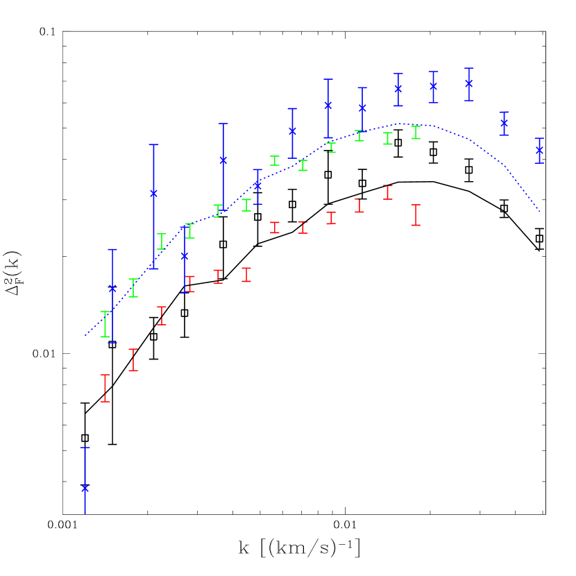
We see large discrepancies, as we expect from the bad . The point at , is below the prediction (as well as any reasonable extrapolation of the other Kim et al. (2004) points), and the points at increasingly high are generally too high (at the highest , this is a reflection of disagreement with the other high resolution data, but actually the agreement is not much better if we only include SDSS in the fit, because no model can fit the highest SDSS points and then climb to match the higher Kim et al. (2004) points). To reassure the reader that we are not playing games with the fitted curves, we also plot the SDSS points at and 2.6.
Since the Kim et al. (2004) results clearly have some problem, unless the other three measurements are all wrong (we will see that, with one exception, the other three agree with each other), we eliminate them from the rest of the comparison. A fit to SDSS, McDonald et al. (2000), and Croft et al. (2002) gives for dof (still a bad fit). Removing McDonald et al. (2000), reduces by 44.3 (39 points), while removing Croft et al. (2002) reduces by 97.2 (for 65 points this reduction would occur by chance only 0.6% of the time). Figure 38 shows the Croft et al. (2002) points, along with the fit prediction for them.
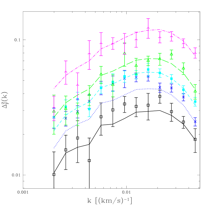
The agreement is actually very good for 4 of the 5 redshift bins, while the points are obviously out of place (these 13 points increase by 54). Figure 39 shows the McDonald et al. (2000) points, along with the fit prediction for them (for this fit we removed the Croft et al. (2002) points).
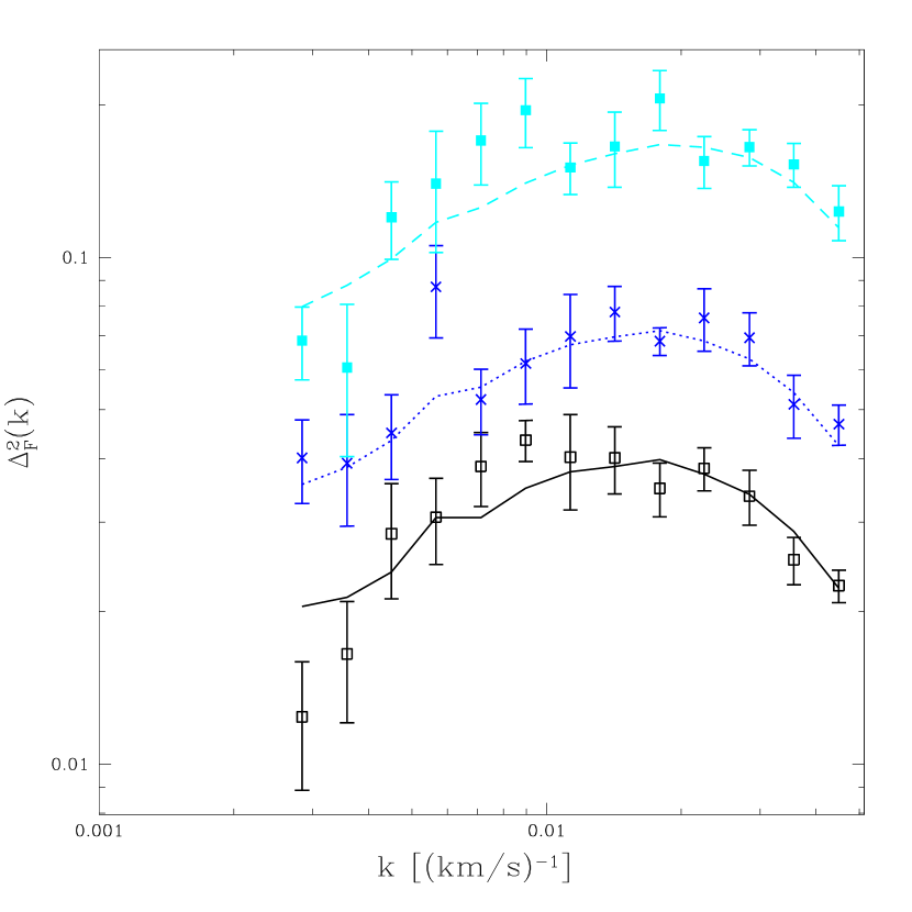
The agreement is good, with the agreement at disfavoring the anomalous Croft et al. (2002) points; further investigation by R. Croft (private communication) does not reveal any obvious error in this redshift bin that would explain the anomaly. Note that the agreement of McDonald et al. (2000) and Croft et al. (2002) at high adds weight to the idea that something is seriously wrong with Kim et al. (2004). Kim et al. (2004) show some comparisons with past results, and claim they agree, but these comparisons used custom redshift bins (i.e., not the bins in their table), and were not high precision (for example they compare the Croft et al. (2002) points at to a bin with , so evolution cancels some of the amplitude offset, and they call the apparent % difference at a “slight” excess).
5 Final Results Table and Directions for Use
Table 3 gives the primary power spectrum results. The columns are: , the redshift of the bin; , the wavenumber of the bin; , our final Ly forest power spectrum result (along with the square roots of the diagonal elements of the error covariance matrix); , the noise power that was subtracted from each bin; and , the background that was subtracted from each bin ( adjusted according to the amount of noise in the forest, eqs. 3, 4, and 13). is just the noise subtracted from (a roughly comparable amount of noise was subtracted from the background, so to some degree these cancel in the final result). The table and the covariance matrix of the errors are available at http://feynman.princeton.edu/pmcdonal/LyaF/sdss.html. The covariance matrix must be used in any serious quantitative fitting. When using this table to constrain models, the following allowances should be made for residual systematic uncertainties:
-
•
Allow % rms error on the noise-power amplitude at each redshift. We do not have any reason to think the error is really this large, but, considering the complications related to the noise, we think it is prudent to include it. Operationally, we suggest subtracting from , where are free parameters in the fit (one for each redshift bin), and adding to .
-
•
Allow rms overall error on the resolution variance (i.e., the square of the rms width of the Gaussian resolution kernel). This is the expected size of the uncertainty due to flexure in the detector, although Figure 5 suggests that it may actually be smaller. Specifically, multiply by , with a free parameter in the fit, and add to .
-
•
SiIII-Ly cross-correlation must be accounted for. We have suggested a simple method – assume the cross-correlation has the same form as the Ly-Ly auto-correlation up to an amplitude that is a free parameter, and possibly include freedom in the correlation width and/or redshift evolution of the amplitude – but others could be devised (e.g., including SiIII in the simulated spectra through a parameterized semi-analytic model).
| 2.2 | 0.00141 | 6.20 | 3.29 | |
| 2.2 | 0.00178 | 6.07 | 2.71 | |
| 2.2 | 0.00224 | 6.20 | 2.46 | |
| 2.2 | 0.00282 | 6.23 | 2.45 | |
| 2.2 | 0.00355 | 5.92 | 1.97 | |
| 2.2 | 0.00447 | 5.57 | 1.18 | |
| 2.2 | 0.00562 | 5.85 | 1.04 | |
| 2.2 | 0.00708 | 5.87 | 1.17 | |
| 2.2 | 0.00891 | 6.06 | 1.20 | |
| 2.2 | 0.01122 | 6.87 | 1.40 | |
| 2.2 | 0.01413 | 8.48 | 1.32 | |
| 2.2 | 0.01778 | 10.52 | 0.87 | |
| 2.4 | 0.00141 | 5.70 | 3.72 | |
| 2.4 | 0.00178 | 5.65 | 2.63 | |
| 2.4 | 0.00224 | 5.65 | 2.45 | |
| 2.4 | 0.00282 | 5.58 | 2.47 | |
| 2.4 | 0.00355 | 5.31 | 1.82 | |
| 2.4 | 0.00447 | 5.15 | 1.18 | |
| 2.4 | 0.00562 | 5.43 | 0.79 | |
| 2.4 | 0.00708 | 5.32 | 1.07 | |
| 2.4 | 0.00891 | 5.71 | 1.14 | |
| 2.4 | 0.01122 | 6.27 | 1.29 | |
| 2.4 | 0.01413 | 7.32 | 1.22 | |
| 2.4 | 0.01778 | 9.37 | 0.91 | |
| 2.6 | 0.00141 | 6.78 | 4.02 | |
| 2.6 | 0.00178 | 6.68 | 3.18 | |
| 2.6 | 0.00224 | 6.76 | 2.65 | |
| 2.6 | 0.00282 | 6.63 | 2.41 | |
| 2.6 | 0.00355 | 6.52 | 1.79 | |
| 2.6 | 0.00447 | 6.40 | 1.27 | |
| 2.6 | 0.00562 | 6.69 | 1.05 | |
| 2.6 | 0.00708 | 6.71 | 1.17 | |
| 2.6 | 0.00891 | 7.12 | 1.05 | |
| 2.6 | 0.01122 | 7.91 | 1.24 | |
| 2.6 | 0.01413 | 9.15 | 1.22 | |
| 2.6 | 0.01778 | 11.66 | 0.95 | |
| 2.8 | 0.00141 | 6.83 | 2.99 | |
| 2.8 | 0.00178 | 6.75 | 2.10 | |
| 2.8 | 0.00224 | 6.79 | 1.84 | |
| 2.8 | 0.00282 | 6.78 | 2.29 | |
| 2.8 | 0.00355 | 6.60 | 1.52 | |
| 2.8 | 0.00447 | 6.52 | 1.22 | |
| 2.8 | 0.00562 | 6.73 | 1.19 | |
| 2.8 | 0.00708 | 6.95 | 0.98 | |
| 2.8 | 0.00891 | 7.41 | 1.11 | |
| 2.8 | 0.01122 | 8.06 | 1.18 | |
| 2.8 | 0.01413 | 9.37 | 1.13 | |
| 2.8 | 0.01778 | 11.64 | 0.90 | |
| 3.0 | 0.00141 | 7.76 | 3.51 | |
| 3.0 | 0.00178 | 7.63 | 2.74 | |
| 3.0 | 0.00224 | 7.73 | 2.20 | |
| 3.0 | 0.00282 | 7.66 | 2.84 | |
| 3.0 | 0.00355 | 7.51 | 1.81 | |
| 3.0 | 0.00447 | 7.34 | 1.30 | |
| 3.0 | 0.00562 | 7.56 | 1.33 | |
| 3.0 | 0.00708 | 7.63 | 0.99 | |
| 3.0 | 0.00891 | 8.15 | 1.30 | |
| 3.0 | 0.01122 | 8.83 | 1.30 | |
| 3.0 | 0.01413 | 9.89 | 1.38 | |
| 3.0 | 0.01778 | 11.90 | 0.91 | |
| 3.2 | 0.00141 | 9.57 | 5.07 | |
| 3.2 | 0.00178 | 9.44 | 3.73 | |
| 3.2 | 0.00224 | 9.46 | 3.01 | |
| 3.2 | 0.00282 | 9.38 | 2.59 | |
| 3.2 | 0.00355 | 9.28 | 2.71 | |
| 3.2 | 0.00447 | 8.95 | 1.36 | |
| 3.2 | 0.00562 | 9.15 | 1.28 | |
| 3.2 | 0.00708 | 9.40 | 1.29 | |
| 3.2 | 0.00891 | 9.80 | 1.48 | |
| 3.2 | 0.01122 | 10.49 | 1.80 | |
| 3.2 | 0.01413 | 11.74 | 1.38 | |
| 3.2 | 0.01778 | 14.07 | 1.18 | |
| 3.4 | 0.00141 | 11.12 | 4.08 | |
| 3.4 | 0.00178 | 11.32 | 2.41 | |
| 3.4 | 0.00224 | 10.97 | 2.09 | |
| 3.4 | 0.00282 | 11.04 | 3.16 | |
| 3.4 | 0.00355 | 10.96 | 2.62 | |
| 3.4 | 0.00447 | 10.76 | 2.00 | |
| 3.4 | 0.00562 | 10.99 | 2.04 | |
| 3.4 | 0.00708 | 11.28 | 1.55 | |
| 3.4 | 0.00891 | 11.87 | 1.77 | |
| 3.4 | 0.01122 | 13.06 | 2.00 | |
| 3.4 | 0.01413 | 14.63 | 1.63 | |
| 3.4 | 0.01778 | 17.80 | 1.23 | |
| 3.6 | 0.00141 | 15.11 | 2.25 | |
| 3.6 | 0.00178 | 14.90 | 2.87 | |
| 3.6 | 0.00224 | 14.87 | 3.28 | |
| 3.6 | 0.00282 | 14.51 | 3.30 | |
| 3.6 | 0.00355 | 14.59 | 2.26 | |
| 3.6 | 0.00447 | 14.22 | 1.33 | |
| 3.6 | 0.00562 | 14.17 | 1.28 | |
| 3.6 | 0.00708 | 14.41 | 1.62 | |
| 3.6 | 0.00891 | 15.09 | 1.98 | |
| 3.6 | 0.01122 | 15.72 | 1.61 | |
| 3.6 | 0.01413 | 17.26 | 1.25 | |
| 3.6 | 0.01778 | 21.11 | 1.51 | |
| 3.8 | 0.00141 | 22.58 | 6.89 | |
| 3.8 | 0.00178 | 20.93 | 6.40 | |
| 3.8 | 0.00224 | 20.91 | 5.07 | |
| 3.8 | 0.00282 | 20.76 | 2.20 | |
| 3.8 | 0.00355 | 21.00 | 2.51 | |
| 3.8 | 0.00447 | 20.37 | 2.37 | |
| 3.8 | 0.00562 | 20.78 | 2.61 | |
| 3.8 | 0.00708 | 21.63 | 2.79 | |
| 3.8 | 0.00891 | 21.69 | 2.57 | |
| 3.8 | 0.01122 | 23.43 | 2.69 | |
| 3.8 | 0.01413 | 26.14 | 2.47 | |
| 3.8 | 0.01778 | 33.51 | 2.15 |
Note. — has units , power spectra have units . The error covariance matrix must be used for any quantitative fitting.
6 Conclusions
We have analyzed a sample of 3035 quasar spectra measured by SDSS and covering the redshift range . This data set is almost two orders of magnitude larger than previously available data sets. We have focused on the flux power spectrum in the redshift range and for modes . The extraordinary size of the data sample leads to an order of magnitude reduction in errors compared to previous analyses. Consequently, to do justice to this data set requires a much more careful analysis than was needed in the past. To this end we have developed a new analysis pipeline using quadratic power spectrum estimation with near optimal performance. We applied this analysis to realistic mock spectra and demonstrated (after several tweaks) that the method performs as expected. We emphasize that realistic mock spectra are essential if one is to trust the results at the level of precision allowed by this data set. Our error estimation is based on bootstrap resampling, which works well here because the individual quasars are independent of each other. The errors were tested against mock spectra and found to be accurate. We also compared the bootstrap errors to Gaussian errors, finding them to be in general less than 20% higher than Gaussian.
Given the small errors on the recovered flux power spectrum the required control of systematic effects must be improved correspondingly as well. A significant part of this paper is devoted to this issue. We find several sources of contamination present in the data and develop methods to remove them. Metal absorption for metals with rest wavelength transitions above Å, uncertainties in sky subtraction, and calibration errors can be subtracted essentially exactly by measuring the power on the red side of Ly forest using the same observed wavelength range. We search for a contribution from metals with transitions close to Ly- using a correlation function analysis, assuming that they are correlated with hydrogen. We find clear evidence of SiIII contamination and develop a simple and effective scheme to remove it. This procedure improves the of the fit from 194 to 129 for degrees of freedom and is thus necessary for a satisfactory fit. We find no evidence of any other metal line contribution to the background subtracted flux power spectrum.
We reduce any contribution of the continuum to the flux power spectrum by dividing each spectrum by the mean quasar continuum. If contributions from quasar-to-quasar continuum differences are similar in different regions of the spectrum, then our subtraction of power from the red side of Ly, as described above, should remove them. Several tests suggest that any residual contributions from continuum fluctuations are negligible. First, we measure the power in the mean continuum in several rest frame regions, finding it to be always small relative to our error bars, so power in quasar-to-quasar fluctuations has to be larger than power in the mean continuum itself to be significant. Second, measurements of the background in several rest frame regions place upper limits on the fluctuations in those regions. Third, a split of the Ly forest region into two halves reveals no evidence that residual continuum fluctuations differ from one half to the other. Finally, estimating the continuum quasar-by-quasar using a principal component analysis does not change the power spectrum results significantly.
In section §4 we perform a series of tests to verify the robustness of the analysis against several modifications of the standard procedure and splits of the data. This reveals an interesting correlation between the power in the red side and the average noise (and some other properties of the spectra that correlate with noise, like the amplitude of the sky flux relative to the quasar flux). While we do not have a detailed explanation for this effect, we are able to remove it by modifying the standard procedure to include this correlation. From our full battery of tests, we conclude that systematic effects in the power spectrum measurement are not likely to significantly affect the results of cosmological fitting (i.e., it is likely that some effects remain formally significant relative to the errors on , but the shape of these systematic errors does not seem to correspond to a change in the cosmological parameters). This conclusion is further confirmed by the analysis of different subsets, which do not reveal any systematic deviations from those expected statistically.
In this paper we limit ourselves to the analysis of the flux power spectrum, without attempting to compare it to cosmological models. The results of this paper should thus be fairly noncontroversial and can be used by others who wish to perform their own cosmological analysis. Our own analysis will be presented in a separate publication, as will the cosmological implications that follow from it. We note that the expected error on the linear rms amplitude of fluctuations is % and on the slope is , both at the pivot point . This should be compared to 10% error on the amplitude and 0.04 on the slope from the WMAP data at (Spergel et al., 2003). This data set provides very tight constraints on the amplitude and slope of the matter power spectrum. Many additional analyses can be performed using this data set, among them the mean flux evolution, cross-correlations between close pairs, and a bispectrum measurement. These will provide a wealth of additional information both on cosmology and on the state of the intergalactic medium at , and they will allow us to test the basic picture of the Ly forest that has emerged over the last decade. We believe that the unprecedented size of this data set will revolutionize our understanding of the high redshift universe; this work is merely a first step in this endeavor.
References
- Abazajian et al. (2003) Abazajian, K., et al. 2003, AJ, 126, 2081
- Abazajian et al. (2004) Abazajian, K., et al. 2004, astro-ph/0403325
- Bernardi et al. (2003) Bernardi, M., et al. 2003, AJ, 125, 32
- Bi et al. (1992) Bi, H. G., Boerner, G., & Chu, Y. 1992, A&A, 266, 1
- Blanton et al. (2003) Blanton, M. R., Lin, H., Lupton, R. H., Maley, F. M., Young, N., Zehavi, I., & Loveday, J. 2003, AJ, 125, 2276
- Cen et al. (1994) Cen, R., Miralda-Escude, J., Ostriker, J. P., & Rauch, M. 1994, ApJ, 437, L9
- Croft et al. (2002) Croft, R. A. C., Weinberg, D. H., Bolte, M., Burles, S., Hernquist, L., Katz, N., Kirkman, D., & Tytler, D. 2002, ApJ, 581, 20
- Croft et al. (1998) Croft, R. A. C., Weinberg, D. H., Katz, N., & Hernquist, L. 1998, ApJ, 495, 44
- Fukugita et al. (1996) Fukugita, M., Ichikawa, T., Gunn, J. E., Doi, M., Shimasaku, K., & Schneider, D. P. 1996, AJ, 111, 1748
- Gnedin & Hamilton (2002) Gnedin, N. Y., & Hamilton, A. J. S. 2002, MNRAS, 334, 107
- Gnedin & Hui (1998) Gnedin, N. Y., & Hui, L. 1998, MNRAS, 296, 44
- Gunn et al. (1998) Gunn, J. E., et al. 1998, AJ, 116, 3040
- Hall et al. (2002) Hall, P. B., et al. 2002, ApJS, 141, 267
- Hernquist et al. (1996) Hernquist, L., Katz, N., Weinberg, D. H., & Jordi, M. 1996, ApJ, 457, L51
- Hogg et al. (2001) Hogg, D. W., Finkbeiner, D. P., Schlegel, D. J., & Gunn, J. E. 2001, AJ, 122, 2129
- Kim et al. (2003) Kim, T. ., Viel, M., Haehnelt, M. G., Carswell, R. F., & Cristiani, S. 2003, ArXiv Astrophysics e-prints
- Kim et al. (2004) Kim, T.-S., Viel, M., Haehnelt, M. G., Carswell, R. F., & Cristiani, S. 2004, MNRAS, 347, 355
- Lynds (1971) Lynds, R. 1971, ApJ, 164, L73
- Mandelbaum et al. (2003) Mandelbaum, R., McDonald, P., Seljak, U., & Cen, R. 2003, MNRAS, 344, 776
- McDonald et al. (2001) McDonald, P., Miralda-Escudé, J., Rauch, M., Sargent, W. L. W., Barlow, T. A., & Cen, R. 2001, ApJ, 562, 52
- McDonald et al. (2000) McDonald, P., Miralda-Escudé, J., Rauch, M., Sargent, W. L. W., Barlow, T. A., Cen, R., & Ostriker, J. P. 2000, ApJ, 543, 1
- Pier et al. (2003) Pier, J. R., Munn, J. A., Hindsley, R. B., Hennessy, G. S., Kent, S. M., Lupton, R. H., & Ivezić, Ž. 2003, AJ, 125, 1559
- Richards et al. (2002) Richards, G. T., et al. 2002, AJ, 123, 2945
- Ricotti et al. (2000) Ricotti, M., Gnedin, N. Y., & Shull, J. M. 2000, ApJ, 534, 41
- Schaye et al. (2003) Schaye, J., Aguirre, A., Kim, T., Theuns, T., Rauch, M., & Sargent, W. L. W. 2003, ApJ, 596, 768
- Schaye et al. (2000) Schaye, J., Theuns, T., Rauch, M., Efstathiou, G., & Sargent, W. L. W. 2000, MNRAS, 318, 817
- Seljak (1998) Seljak, U. . 1998, ApJ, 506, 64
- Seljak et al. (2003) Seljak, U., McDonald, P., & Makarov, A. 2003, MNRAS, 342, L79
- Slanger et al. (2003) Slanger, T. G., Cosby, P. C., Osterbrock, D. E., Stone, R. P. S., & Misch, A. A. 2003, PASP, 115, 869
- Smith et al. (2002) Smith, J. A., et al. 2002, AJ, 123, 2121
- Spergel et al. (2003) Spergel, D. N., et al. 2003, ApJS, 148, 175
- Stoughton et al. (2002) Stoughton, C., et al. 2002, AJ, 123, 485
- Tegmark (1997) Tegmark, M. 1997, Phys. Rev. D, 55, 5895
- Tegmark et al. (1997) Tegmark, M., Taylor, A. N., & Heavens, A. F. 1997, ApJ, 480, 22
- Theuns et al. (1998) Theuns, T., Leonard, A., Efstathiou, G., Pearce, F. R., & Thomas, P. A. 1998, MNRAS, 301, 478
- Vogt et al. (1994) Vogt, S. S., et al. 1994, in Proc. SPIE Instrumentation in Astronomy VIII, David L. Crawford; Eric R. Craine; Eds., Volume 2198, p. 362, Vol. 2198
- York et al. (2000) York, D. G., et al. 2000, AJ, 120, 1579
- Zaldarriaga et al. (2001) Zaldarriaga, M., Scoccimarro, R., & Hui, L. 2001, ApJ, submitted (astro-ph/0111230)
- Zhang et al. (1995) Zhang, Y., Anninos, P., & Norman, M. L. 1995, ApJ, 453, L57