Inferring the dark matter power spectrum from the Lyman-$\alpha$ forest in high-resolution QSO absorption spectra

Abstract

We use the LUQAS sample (Kim et al. 2004), a set of 27 high-resolution and high signal-to-noise QSO absorption spectra at a median redshift of $z=2.25$, and the data from Croft et al. (2002) at a median redshift of $z=2.72$, together with a large suite of high-resolution large box-size hydro-dynamical simulations, to estimate the linear dark matter power spectrum on scales $0.003\,{\rm s/km}<k<0.03\,{\rm s/km}$. Our re-analysis of the Croft et al. data agrees well with their results if we assume the same mean optical depth and gas temperature-density relation. The inferred linear dark matter power spectrum at $z=2.72$ also agrees with that inferred from LUQAS at lower redshift if we assume that the increase of the amplitude is due to gravitational growth between these redshifts. We further argue that the smaller mean optical depth measured from high-resolution spectra is more accurate than the larger value obtained from low-resolution spectra by Press et al. (1993) which Croft et al. used. For the smaller optical depth we obtain a $\approx 20$% higher value for the rms fluctuation amplitude of the matter density. By combining the amplitude of the matter power spectrum inferred from the Ly$\alpha$ forest with the amplitude on large scales inferred from measurements of the CMB we obtain constraints on the primordial spectral index $n$ and the normalisation $\sigma_{8}$. For values of the mean optical depth favoured by high-resolution spectra, the inferred linear power spectrum is consistent with a $\Lambda$CDM model with a scale-free ($n=1$) primordial power spectrum.

1 Introduction

The prominent absorption features blue-ward of the Lyman-$\alpha$ emission in the spectra of high-redshift quasars (QSOs) are now generally believed to arise from smooth density fluctuations of a photoionised warm intergalactic medium (see Rauch 1998 and Weinberg et al. 1999 for reviews). This has opened up the possibility to probe the density fluctuation of matter with the flux power spectrum of QSO absorption lines (Croft et al. 1998, Hui 1999, Croft et al. 1999b, McDonald et al. 2000 [M00], Hui et al. 2001, Croft et al. 2002 [C02], McDonald 2003, Viel et al. 2003).

The flux power spectrum is mainly sensitive to the slope and amplitude of the linear dark matter power spectrum for wave-numbers in the range $0.002\,{\rm s/km}<k<0.05\,{\rm s/km}$. Croft et al. (1999) inferred an amplitude and slope which was consistent with a COBE normalised $\Lambda$CDM model with a primordial scale invariant fluctuation spectrum (Phillips et al. 2001). M00 and C02, using a larger sample of better quality data, found a somewhat shallower slope and smaller fluctuation amplitude. The WMAP team used the later data in combination with their CMB data to claim that there is evidence for a tilted primordial CMB-normalised fluctuation spectrum ($n<1$) and/or a running spectral index (Bennet et al. 2003; Spergel et al. 2003; Verde et al. 2003). A number of authors have argued that the errors in the inferred dark matter (DM) power spectrum have been underestimated (Zaldarriaga, Scoccimarro & Hui, 2003; Zaldarriaga, Hui & Tegmark, 2001; Gnedin & Hamilton 2002; Seljak, McDonald & Makarov 2003). We here use a suite of high-resolution hydro-dynamical simulations and the flux power spectrum obtained from LUQAS (Large Sample of UVES QSO Absorption Spectra), together with the published flux power spectrum of C02 to further investigate these issues.

The plan of the paper is as follows. In Section 2 we describe the two data sets and give an overview of the determinations of the effective optical depth found in the literature. The flux power spectra obtained from the hydro-dynamical simulations are discussed in Section 3. Section 4 describes the method and uncertainties of inferring the linear matter power spectrum. In Section 5 we present our results, compare with previous results and discuss implications for $\sigma_{8}$ and $n$. Section 6 contains a summary and our conclusions.

2 The observed flux power spectrum and effective optical depth

We will use estimates of the flux power spectrum from two different data sets: the LUQAS sample of VLT spectra compiled by K04 and the sample of Keck spectra compiled by C02. Below, we will describe both samples in more detail.

2.1 The LUQAS sample

LUQAS (Large Sample of UVES Quasar Absorption Spectra) compiled by K04, consists of 27 high-resolution spectra taken with the VLT UVES spectrograph. The median redshift of the Lyman-$\alpha$ forest probed by the spectra is $\left<z\right>=2.25$ and the total redshift path covered is $\Delta z=13.75$. The S/N varies as a function of wavelength, but in the forest region it is usually larger than 50. The flux power spectrum of the LUQAS sample has been analysed in K04, while a study of the flux bispectrum can be found in Viel et al. (2004b).

The LUQAS sample probes somewhat smaller redshifts than the C02 sample, but, as discussed by K04, in the redshift range where the two samples overlap, the estimated flux power spectra agree well in the range of wavenumbers not affected by differences in resolution and S/N. Here, we will use a subset of the LUQAS sample for which we have selected all QSO spectra regions in the redshift range $2<z<2.3$, to maximise the contrast in redshift to the C02 sample and to further investigate the redshift evolution. 16 QSOs contribute to this subsample (Figure 1 in K04) and the median redshift is $\left<z\right>=2.125$. In Table 1, we give the 3D flux power spectrum $\Delta^{2}_{F}(k)=P_{F}^{\rm 3D}(k)\,k^{3}/(2\pi^{2})$ for this sample, using the flux estimator $F/\left<F\right>-1$ (denoted $F2$ in K04), where $F$ is the flux of the continuum-fitted spectra. The 3D flux power spectrum is obtained from the 1D flux power spectrum by differentiation in the usual way, viz.

$$P^{\rm 3D}_{F}=-\frac{2\,\pi}{k}\frac{{\rm d}P^{\rm 1D}_{F}}{{\rm d}k}\;.$$ (1)

Note that peculiar velocities and thermal broadening make the flux field anisotropic and that $P_{F}^{\rm 3D}$ is thus not the true 3D power spectrum of the flux. The flux power spectrum has been calculated for the same wavenumbers as in C02.

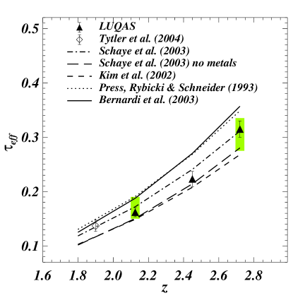
Figure 1: Triangles show the effective optical depth $\tau_{\rm eff}=-\ln\left<F\right>$ for the LUQAS sample (also given in Table 2). The dashed curve is the result of Kim et al. (2002) while the long-dashed and dot-dashed curves show the result of Schaye et al. (2003), with and without the removal of pixels contaminated by metals, respectively. The dotted curve is the effective optical depth obtained by Press, Rybicki & Schneider (1993). The solid curve shows the results from Bernardi et al. (2003). The empty diamond is the result of Tytler et al. (2004). The vertical extent of the two shaded regions indicates the values used in our analysis.

2.2 The Croft et al. sample

The Croft et al. (2002) sample (C02) consists of 30 Keck HIRES spectra and 23 Keck LRIS spectra. We will here use the flux power spectrum which C02 derived for what they call their ‘fiducial’ sample. This sample has a median redshift $\left<z\right>=2.72$, spans the redshift range $2.3<z<3.2$, and has a total redshift path of $\Delta z=25$. For more details see C02.

Table 1: The 1D and 3D power spectrum of the flux $F=\exp(-\tau)/\left<\exp(-\tau)\right>-1$ of the LUQAS sample at $z=2.125$.

$k$ (s/km)	$P^{\rm 1D}_{F}(k)$ (s/km)	$\Delta^{2}_{F}(k)$
0.00199	18.4942 $\pm$ 2.9106	0.0002 $\pm$ 0.0031
0.00259	16.6206 $\pm$ 2.7119	0.0003 $\pm$ 0.0040
0.00336	21.0862 $\pm$ 3.3361	0.0004 $\pm$ 0.0052
0.00436	16.2223 $\pm$ 1.7413	0.0106 $\pm$ 0.0039
0.00567	13.9062 $\pm$ 1.2669	0.0153 $\pm$ 0.0075
0.00736	12.9220 $\pm$ 2.3890	0.0194 $\pm$ 0.0077
0.00956	9.6921 $\pm$ 0.9864	0.0156 $\pm$ 0.0065
0.01242	8.9783 $\pm$ 0.7195	0.0253 $\pm$ 0.0065
0.01614	7.2158 $\pm$ 0.5574	0.0421 $\pm$ 0.0037
0.02097	4.4987 $\pm$ 0.2800	0.0499 $\pm$ 0.0054
0.02724	3.3617 $\pm$ 0.2313	0.0468 $\pm$ 0.0055
0.03538	2.1198 $\pm$ 0.1135	0.0498 $\pm$ 0.0054
0.04597	1.1490 $\pm$ 0.0677	0.0424 $\pm$ 0.0032
0.05971	0.6303 $\pm$ 0.0480	0.0345 $\pm$ 0.0030
0.07757	0.2833 $\pm$ 0.0169	0.0256 $\pm$ 0.0022

Table 2: Mean flux and effective optical depth of the LUQAS sample.

redshift range	$\left<z\right>$	$\left<F\right>$	$\tau_{\rm eff}$
$2.0<z<2.3$	2.125	$0.849\pm 0.008$	$0.163\pm{0.009}$
$2.3<z<2.6$	2.44	$0.800\pm 0.008$	$0.223\pm{0.014}$
$2.55<z<3.0$	2.72	$0.730\pm 0.011$	$0.315\pm{0.015}$

2.3 Statistical and systematic errors in the observed flux power spectrum

Unless stated otherwise, we estimate our statistical errors with a jack-knife estimator. The main systematic errors affecting estimates of the flux power spectrum due to absorption by the Lyman-$\alpha$ forest are continuum fitting and the presence of metal lines and damped Lyman-$\alpha$ systems. These effects have been investigated by e.g. C02 and K04. The main conclusions of K04 are as follows: i) continuum fitting uncertainties for high-resolution Echelle spectra strongly affect the flux power spectrum at scales $k<0.003\,{\rm s/km}$; ii) the contribution of metal lines is less than 10% at scales $k<0.01\,{\rm s/km}$ but rises significantly (up to 50%) at smaller scales; iii) damped Lyman-$\alpha$ systems appear to only mildly affect the estimate of the flux power spectrum. In order to minimise uncertainties due to continuum fitting and metal lines, and to avoid dealing with the problematic thermal cut-off at small scales, we will only use the range of wavenumbers $0.003<k\,{\rm(s/km)}<0.03$ for our analysis.

2.4 The observed effective optical depth

As pointed out by Croft et al. (1998), C02 and Seljak, McDonald & Makarov (2003) and discussed in detail in Sections 4 and 4.2, the assumed effective optical depth, $\tau_{\rm eff}=-\ln{\left<F\right>}\,$, has a large influence on the amplitude of the inferred matter power spectrum. The observed values of $\tau_{\rm eff}$ have large statistical and probably also not yet fully understood systematic errors. The main uncertainty in determining the effective optical depth comes from the continuum fitting procedure and the Poisson noise due to the large variations from line-of-sight to line-of-sight (Zuo & Bond 1994, Viel et al. 2004a, Tytler et al. 2004).

In Figure 1, we show results for the redshift evolution of $\tau_{\rm eff}$ from a number of observational studies in the literature. The dotted curve is from a large sample of low-resolution spectra compiled by Press, Rybicki & Schneider (1993, PRS), while the solid line is from a sample of low resolution spectra drawn from SDSS by Bernardi et al. (2003). The open diamond shows the result from Tytler et al. (2004). The short-dashed curve is the result of Kim et al. (2002) using a sample of high-resolution UVES spectra, while the long-dashed and dash-dotted curves show the results of Schaye et al. (2003) from a combined sample of high-resolution UVES and Keck spectra with and without the removal of pixels contaminated by associated metal absorption. The filled triangles show the results from the LUQAS sample for three different redshift ranges (also given in Table 2). Damped and sub-damped Lyman-$\alpha$ systems have been removed for the estimate from the LUQAS sample and errors have been calculated with a jack-knife estimate using 40 subsamples. Note that the sample used by Schaye et al. (2003) has 14 QSO spectra in common with the LUQAS sample.

The results of PRS and Bernardi et al. (2003), which both use low-resolution spectra with comparably low S/N, give results which are about 15-20% higher than those of studies using high-resolution spectra (see also Schaye et al. 2003 for a discussion). As argued by Seljak et al. (2003) and Tytler et al. (2004) this is most likely due to systematic errors in the continuum fitting procedure of the low-resolution spectra. We agree with this assessment. At redshifts $\leq 2.7$ the expected continuum fitting errors in high-resolution spectra is of order 2% (Bob Carswell and Tae-Sun Kim, private communication). For spectra at these redshifts, the errors are thus almost certainly dominated by the somewhat uncertain contribution from metal lines and statistical errors. Based on Figure 1 we will adopt the following values for the optical depth and its error in our further analysis, $\tau_{\rm eff}(z=2.125)=0.17\pm 0.02$ and $\tau_{\rm eff}(z=2.72)=0.305\pm 0.030$.

3 The flux power spectrum of simulated absorption spectra

3.1 Numerical code and parameters

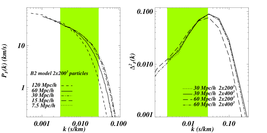
Figure 2: Left panel: 1D flux power spectra of different simulations of model B2 at $z=2.75$, run with different box-sizes. All simulations are with 200³ dark matter particles and 200³ gas particles. Note that simulations have not been scaled to the same effective optical depth. The shaded region indicates the range of wavenumbers used to infer the linear dark matter power spectrum. Right panel: 3D flux power spectra for different simulations of model B2, for a range of box-sizes and resolutions, as indicated in the plot.

Table 3: Grid of cosmological simulation parameters.

	$\sigma_{8}=0.7$	$\sigma_{8}=0.85$	$\sigma_{8}=1.0$
$n=0.95$	B1	B2	B3
$n=1.0$	C1	C2	C3

We have run a suite of simulations with varying cosmological parameters, particle numbers, resolution, boxsize and thermal histories using a new version of the parallel TreeSPH code GADGET (Springel, Yoshida & White, 2001). GADGET-2 was used in its TreePM mode which speeds up the calculation of long-range gravitational forces considerably. The simulations were performed with periodic boundary conditions with an equal number of dark matter and gas particles and used the conservative ‘entropy-formulation’ of SPH proposed by Springel & Hernquist (2002). Radiative cooling and heating processes were followed using an implementation similar to that of Katz et al. (1996) for a primordial mix of hydrogen and helium. We have assumed a mean UV background produced by quasars as given by Haardt & Madau (1996), which leads to reionisation of the Universe at $z\simeq 6$, but have also run simulations where we artificially increased the heating rates to mimic different thermal histories. Most simulations were run with heating rates increased by a factor of 3.3 in order to achieve temperatures which are close to observed temperatures (Schaye et al. 2000; Ricotti et al. 2000; Choudhury, Srianand & Padmanabhan 2001).

In order to maximise the speed of the simulations we have employed a simplified star-formation criterion in the majority of our runs. All gas at densities larger than 1000 times the mean density was turned into collisionless stars. The absorption systems producing the Lyman-$\alpha$ forest have small overdensity so this criterion has little effect on flux statistics, while speeding up the calculation by a factor of $\sim 6$, because the small dynamical times that would otherwise arise in the highly overdense gas need not to be followed any more. In a pixel-to-pixel comparison with a simulation which adopted the full multi-phase star formation model of Springel & Hernquist (2003) we explicitly checked for any differences introduced by this approximation. We found that the differences in the flux probability distribution function were smaller than 2%, while the differences in the flux-power spectrum were smaller than 0.2 %. We have also turned off all feedback options of GADGET-2 in our simulations. The effect of feedback by galactic winds on the statistics of the flux distribution is uncertain but is believed to be small (e.g. Theuns et al. 2002, Bruscoli et al. 2003, Croft et al. 2003, Kollmeier et al. 2003, Desjacques et al. 2004).

The simulations were all started at $z=99$ and we have stored 19 redshift outputs for each run, mainly in the redshift range $1.5<z<3.5$. The initial gas temperature was $T=227$ K, and $40\pm 2$ SPH neighbours were used to compute physical quantities. The gravitational softening was set to 2.5 $h^{-1}$ kpc in comoving units for all particles.

We have run a suite of simulations with cosmological parameters close to the values obtained by the WMAP team in their analysis of WMAP and other data (Spergel et al. 2003), as shown in Table 3. Our fiducial model is a ‘concordance’ $\Lambda$CDM model with $\Omega_{0{\rm m}}=0.26$, $\Omega_{0\Lambda}=0.74$, $\Omega_{0{\rm b}}=0.0463$ and $H_{0}=72\,{\rm km\,s^{-1}Mpc^{-1}}$ (B2 in Table 3). The CDM transfer functions of all models have been taken from Eisenstein & Hu (1999).

The simulations were run on COSMOS, a shared-memory Altix 3700 with 128 900 MHz Itanium processors hosted at the Department of Applied Mathematics and Theoretical Physics (Cambridge), and a 64-node Beowulf cluster with 64 1.2 GHz Sun processors hosted at the Institute of Astronomy (Cambridge). The majority of our simulations have been run with $2\times 400^{3}$ particles in a 60 $h^{-1}$ Mpc  box and they took about 280 hrs on 32 processors to reach $z=2$.

3.2 The effect of resolution and box size on the flux power spectrum

As discussed in K04 and C02 and in Section 2.3, the range of wavenumbers $0.003<k/{\rm(s/km)}<0.03$ is least affected by systematic uncertainties. We will thus limit our attempts to infer the linear dark matter power spectrum to this range, which is indicated by the shaded region in Figure 2 and following figures. In the left panel of Figure 2, we plot the 1D flux power spectrum for a suite of exploratory runs with fixed particle number $2\times 200^{3}$ for five different box sizes/resolutions. All simulations are for our fiducial cosmology B2 and have been run with the same phases. There is generally good agreement in the overlap regions of the flux power spectrum. At large wavenumbers, the flux power spectrum for simulations with box size $\geq 60\,h^{-1}{\rm Mpc}$, where the gas particle mass is larger than $5\times 10^{7}\,h^{-1}{\rm M}_{\odot}$, is however clearly affected by insufficient resolution.

The right panel of Figure 2 shows the effect of increasing the mass resolution by a factor of eight for the $60\,h^{-1}{\rm Mpc}$ and $30\,h^{-1}{\rm Mpc}$ boxes, corresponding to an increase of the particle number to $2\times 400^{3}$. Plotted is the 3D power spectrum which we will use to infer the linear dark matter power spectrum using the ‘effective bias’ method developed by C02. There is good agreement between the flux power spectra for $k>0.008$ s/km, except at small scales for the 60 $h^{-1}$ Mpc  box with only $2\times 200^{3}$ particles. A box size of 60 $h^{-1}$ Mpc  with $2\times 400^{3}$ particles appears to be a suitable compromise for estimates of the DM power spectrum. It has converged on small scales and will only be moderately affected by cosmic variance on the largest scales (for more discussion see Section 4.2 on errors). For this choice, the mass per dark matter particle is $2\times 10^{8}\,h^{-1}{\rm M}_{\odot}$ and the mass per gas particle is $4.3\times 10^{7}\,h^{-1}M_{\odot}$. Note that this is a significant improvement compared to the simulations of C02 who used 10 dark matter simulations with a box size of 27.77 $h^{-1}$ Mpc  and $160^{3}$ particles.

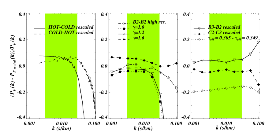
Figure 3: Effect of rescaling simulations (60 $h^{-1}$ Mpc  box $2\times 400^{3}$ particles), to reproduce different temperature-density relations and different values of $\sigma_{8}$. Left: Difference between the 1D flux power spectrum of the ‘hot’ simulation and the rescaled ‘cold’ simulation (solid curve) and vice versa (dashed curve). Middle: Difference between the 1D flux power spectrum of the simulation of the B2 model and the flux power spectra for three rescaled models with different values of the exponent $\gamma$ of the temperature-density relation. The difference between the 1D  flux power spectra of two simulations of model B2 with two different resolutions is also shown (30 $h^{-1}$ Mpc  box, $2\times 400^{3}$ particles). Right: The solid curve shows the difference between the 1D flux power spectra of a simulation of model B2 ($\sigma_{8}=0.85,z=2.72$) and an output of a simulation of model B3 ($\sigma_{8}=1$) at higher redshift which has the same rms density fluctuation (rescaled to the effective optical depth at $z=2.72$). The dashed curve shows the difference between the 1D flux power spectra of a simulation of model C3 ($\sigma_{8}=1.0,z=2.125$) and an output of a simulation of model C2 ($\sigma_{8}=0.85$) at lower redshift which has the same rms density fluctuation (rescaled to the effective optical depth at $z=2.125$). The dotted curve shows the difference between the 1D flux power spectra of a simulation of model B2 for two different values of $\tau_{\rm eff}$. The shaded regions indicate the range of wavenumbers used in our analysis.

3.3 The effect of temperature on the flux power spectrum and the rescaling of the temperature-density relation

It is well established by analytical arguments and numerical simulations that the gas responsible for the Lyman-$\alpha$ forest is in photoionisation equilibrium and exhibits a rather tight relation between density and temperature (e.g. Hui & Gnedin 1997). This relation is a quasi-equilibrium established by the balance between photo-heating and adiabatic cooling. For moderate over-density the relation can be approximated by a power-law of the form,

$$T=T_{0}\left(\frac{\rho}{\left<\rho\right>}\right)^{\gamma-1}.$$ (2)

The slope $\gamma$ and normalisation $T_{0}$ of this relation depend on the reionisation history of the Universe. The effect on the flux power spectrum is twofold. Changing the temperature changes the width of the absorption features and it thus changes the mean flux decrement for a given distribution of neutral hydrogen.

To see how the slope affects the flux power spectrum, it is helpful to consider the fluctuating Gunn-Peterson approximation. The relation between the optical depth and matter density in redshift space can be written as

$$\tau=A\left(\frac{\rho}{\left<\rho\right>}\right)^{\beta},$$ (3)

where $\beta=2.7-0.7\,\gamma$ depends on the temperature-density relation of the gas due to the temperature dependence of the recombination coefficient (see Weinberg et al. 1999 for a review). The factor $A$ depends on redshift, baryon density, temperature at the mean density, Hubble constant and photoionisation rate. Increasing the slope of the temperature-density relation therefore flattens the slope of the relation between optical depth and matter density. At fixed mean optical depth, this results in a decrease of the amplitude of the flux power spectrum.

With a running time of two weeks for each of our simulations we could not afford to run an extensive parameter study of simulations with different thermal histories and temperature-density relations. We have thus used the rescaling method developed by Theuns et al. (1998) to impose a variety of temperature-density relations. This will not account for the effects that the corresponding change in the gas pressure would have had on the gas distribution. It nevertheless mimics the major effects of different density temperature relations on the flux power spectrum reasonably well. To verify this explicitly, we have compared two simulations run with a factor $\sim$ 3.3 different photo-heating rates. The temperatures were different by a factor $\sim 2.5$. The best fitting parameters for the temperature-density relation of the ‘hot’ simulation are $T_{0}=10^{4.15}$ K and $\gamma=1.6$.

In the left panel of Figure 4, we compare the flux power spectra of the ‘hot’ and ‘cold’ simulations with flux power spectra for which the temperatures of the hot/cold simulations have been rescaled such that they have the same temperature-density relation as the cold/hot simulations. The differences between the 1D flux power spectra of rescaled and simulated models are smaller than 10% at small $k$, but start to diverge strongly at $k>0.02\,{\rm s/km}$. The differences mostly depend only weakly on $k$ and the differences between the 3D spectra will generally be smaller. The middle panel shows the effect of rescaling to temperature-density relations with different $\gamma$. We will explore the effect of changing the temperature-density relation on the inferred dark matter power spectrum in more detail in Section 4.

3.4 The amplitude of the matter power spectrum and rescaling of the redshift

Our grid of simulations is somewhat sparse in the fluctuation amplitude of the matter power spectrum. However, at the redshifts considered here, redshift and fluctuation amplitude are largely degenerate and a suitably rescaled simulation output from a different redshift can mimic a simulation with different fluctuation amplitude. In the right panel of Figure 4 we test how well this works by comparing the flux power spectrum of simulations with different $\sigma_{8}$ at redshifts where the rms density fluctuation amplitude of the simulation is the same. The differences at large scales ($k<0.03$ s/km) are typically of the order of 5%.

4 Estimating the matter power spectrum

4.1 The Method

The method we use to infer the linear dark matter power spectrum has been proposed by C02. It uses numerical simulations to calibrate the relation between flux power spectrum and matter power spectrum. It then assumes that the flux power spectrum $P_{F}(k)$ at a given wavenumber $k$ depends linearly on the linear real space matter power spectrum $P(k)$ at the same wavenumber and that both can be related by a simple bias function $b(k)$,

$$P_{F}(k)=b^{2}(k)\,P_{\rm mat}(k)\;.$$ (4)

The flux power spectrum obtained from the hydro-simulations is used to determine $b(k)$. In reality, some mode coupling is expected (Gnedin & Hamilton 2002) and the relation between flux and matter power spectrum will in general not be linear. However, if the true matter power spectrum is close to the matter power spectrum used to determine $b(k)$ the approximation has shown to give accurate results. We refer to C02, Gnedin & Hamilton (2002) and Zaldarriaga, Scoccimarro & Hui (2003) for more details and for an extensive discussion of the possible limitation of this method.

With our grid of models of varying slope and amplitude of the DM power spectrum, we always have a simulation which comes close to reproducing the observed flux power spectrum to within $\sim 10$% in the range $0.003<k$ (s/km) $<0.03$. We then use the $b(k)$ determined from this simulation to infer the ‘observed’ linear matter power spectrum by dividing the observed flux power spectrum by $b^{2}(k)$. The ‘corrections’ of the linear power spectrum with respect to the one actually simulated are smaller than 10%.

Figure 4: $b_{\rm fid}/b$ for three different simulations with different values of $\sigma_{8}$. Left: $b_{\rm fid}/b$ as a function of $\tau_{\rm eff}$ (no scaling of the temperature-density relation has been adopted here). We also show the scaling found by Croft et al. (2002) [C02] and Gnedin & Hamilton (2002) [GH02] as thin solid and dashed curves, respectively. Middle: $b_{\rm fid}/b$ as a function of $T_{0}$, the temperature at the mean density, for a fixed $\tau_{\rm eff}=0.305$ and $\gamma=1.2$. Right: $b_{\rm fid}/b$ as a function of $\gamma$, the power-law index of the temperature-density relation, for a fixed $\tau_{\rm eff}=0.305$ and $T_{0}=10^{4.15}$ K.

4.2 Statistical errors

As discussed in Section 2.4, the systematic uncertainties on the observed flux power spectrum are small for 0.003 s/km $<k<$ 0.03 s/km, the range of wavenumber we have used for our analysis. The errors of the observed flux power spectrum in this range of wavenumbers should be dominated by statistical errors. In the following, we will assume the statistical errors of the inferred linear matter power spectrum to be the same as the statistical errors of the observed flux power spectrum. Cosmic variance in the flux power spectrum of our simulated spectra is a further possible source of statistical error in our modelling. However, our analysis is performed using simulations with a box size of $60$$h^{-1}$ Mpc  which corresponds to 6082.3 km/s in velocity space. Our simulation thus probes a volume which is $\sim 27$ times larger than $(2\pi/k_{\rm min})^{3}$, where $k_{\rm min}=0.003\,{\rm s/km}$ is the smallest wavenumber we use for our analysis. The cosmic variance error due to the finite size of our simulation box should thus only moderately affect the smallest wavenumber we use. Its contribution to the total error of the rms fluctuation amplitude will be negligible compared to the other systematic errors which we describe in the next section.

4.3 Systematic errors

4.3.1 The effective optical depth

The inferred amplitude of the matter power spectrum depends strongly on the assumed effective optical depth of the absorption spectrum (e.g. Croft et. al. 1998; C02; Gnedin & Hamilton 2002; Seljak, McDonald & Makarov 2003). In Figure 4 (right panel), we show the effect of changing the mean optical depth on the 1D flux power spectrum. The dotted curve shows the difference of the 1D flux power spectrum if $\tau_{\rm eff}$ is changed from 0.305 to 0.349 for the B2 simulation. Increasing the mean optical depth increases the flux power spectrum by a factor which is nearly constant for $k<0.03$ s/km.

To quantify the effect of the effective optical depth on the inferred linear matter power spectrum, we consider the ratio $b_{\rm fid}/b$, where $b_{\rm fid}$ is the average value of the bias function $b(k)$ for a fiducial model in the range considered, and $b$ is the average value for a model with different parameters ($\tau_{\rm eff}$, $T_{0}$ and $\gamma$). In Figure 4 (left panel), we show the effect of changing the assumed effective optical depth on the 3D flux power spectrum at small $k$, for three different simulations with three different values of $\sigma_{8}$ at $z=2.75$. The dependence on $\sigma_{8}$ is weak. The dependence of $b_{\rm fid}/b$ on $\tau_{\rm eff}$ is well fitted by

$${b_{\rm fid}\over b}\sim\left({\tau_{\rm eff}\over 0.305}\right)^{-0.7}.$$ (5)

This dependence is intermediate between that found by C02 and that by Gnedin & Hamilton (2002).

4.3.2 The temperature-density relation

The solid, dotted and dashed curves in Figure 3b show the effect of changing $\gamma$ on the 1D flux power spectrum. Increasing $\gamma$ leads to a decrease of the flux power, again by a factor which is nearly constant for $k<0.03$ s/km. In the middle and right panels of Figure 4, we show the dependence of $b_{\rm fid}/b$ on $\gamma$ and $T_{0}$ (averaged over $k$ for $0.003<k/{\rm(s/km)}<0.03$) where $b_{\rm fid}$ is again the ratio of flux to matter power spectrum for our fiducial model. We fixed $\tau_{\rm eff}=0.305$ and rescaled to $\gamma=1.2$ (middle panel) and $T_{0}=10^{4.15}$ K (right panel), respectively. Rescaled ’hot’ simulations were used in all cases.

The dependences of $b_{\rm fid}/b$ on $T_{0}$ and $\gamma$ are fitted by

$${b_{\rm fid}\over b}\sim\left[{1+T_{0}/(10^{4.15}\,{\rm K})\over 2}\right]^{-0.15},$$ (6)

and

$${b_{\rm fid}\over b}\sim\left({1+\gamma/1.3\over 2}\right)^{0.3},$$ (7)

respectively. C02 found a somewhat weaker dependence on the value of $T_{0}$, and no dependence on $\gamma$.

4.3.3 Other systematic errors

Other possible systematic errors include fluctuations of the UV background and potentially modifications of the forest by galactic winds. Variations of the flux of hydrogen ionising photons are expected to be large in the intermediate aftermath of reionisation. However, at the redshifts we are interested in here, they are expected to be small due to the large mean free path of ionising photons. Meiksin & White (2003) estimate that their effect on the flux power spectrum should be smaller than 0.5% at $z=2.75$.

The effect of galactic winds on the flux power spectrum will depend strongly on the volume filling factor of galactic outflows and on when the winds occur (Theuns et al. 2002, Bruscoli et al. 2002). In the range of wavenumbers which we used for our analysis, Croft et al. (2003) and Desjaques et al. (2004) found a negligible effect on the flux power spectrum for galactic winds consistent with the correlation between flux decrement and galaxies detected by Adelberger et al. (2003) at $z\sim 3$, while Weinberg et al. (2003) found a decrease of the flux power at large scales when considering strong winds models. Galactic winds appear to affect the flux power spectrum mainly by their effect on the strong absorption systems which contribute significantly to the flux power spectrum (Viel et al. 2004a).

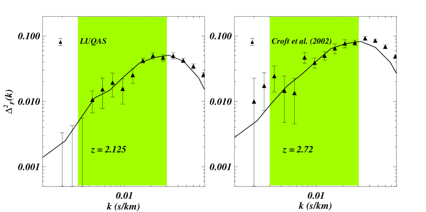
Figure 5: Left: Flux power spectrum at $z=2.125$. The filled triangles are for the LUQAS subsample with a mean redshift of $z=2.125$ (see Table 1). The continuous curve is the power spectrum of the simulation that fits the data best. Right: Flux power spectrum at $z=2.72$. The filled triangles are for the fiducial sample of Croft et al. (2002). The continuous curve is the power spectrum of the simulation that fits the data best (with $\tau_{\rm eff}=0.305$). Shaded regions indicate the range of wavenumbers used in our analysis.

5 The inferred matter power spectrum

5.1 The linear power spectrum from LUQAS and Croft et al.

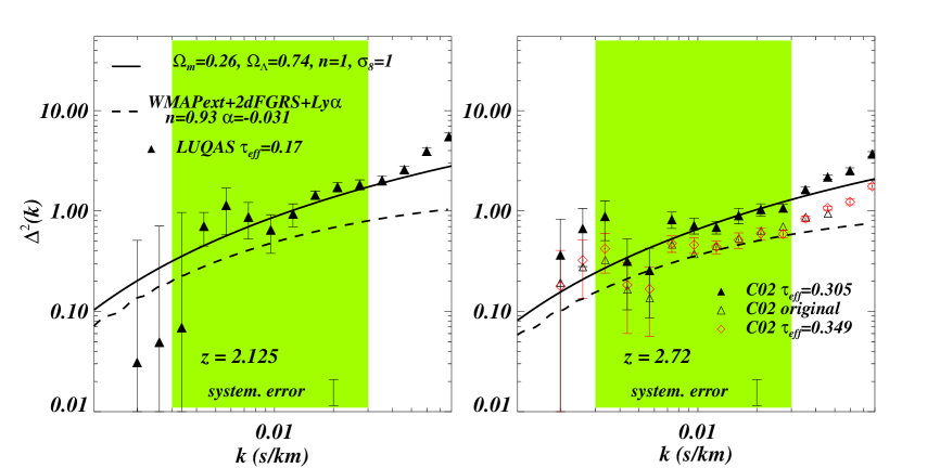
Figure 6: Left: Linear power spectrum at $z=2.125$. The linear dark matter power spectrum inferred from the LUQAS fiducial sample with the bias parameter derived from a simulation of model C3 which fits the data best. The statistical errors are the same as those of the flux power spectrum in Fig. 5. The curve is a theoretical linear power spectrum with parameters as given on the plot. The error bar at the bottom of the plot is our estimate of the systematic uncertainty as discussed in Section 5.2. Shaded regions indicate the range of wavenumbers used in our analysis. Right: Linear power spectrum at $z=2.72$. Empty triangles show the result obtained by C02. Empty diamonds are the result of our analysis for the same optical depth as used by Croft et al. ($\tau_{\rm eff}=0.349$). Solid triangles are the result of our analysis for our preferred effective optical depth of $\tau_{\rm eff}=0.305$. The solid and dashed curves are theoretical linear power spectra with parameters as indicated in the plot. The dashed curve is the “best fitting” model with a running spectral index found by the WMAP team (Spergel et al. 2003).

In this Section, we present the main result of the paper, the linear dark matter power spectrum we infer for the LUQAS and C02 samples. As discussed in Section 4.1, we first have to find the simulation output for which the 3D flux power spectrum fits the observed flux power spectrum best. To this end we have used $\chi^{2}$ minimisation in the range $0.003<k$ (s/km) $<0.03$. For these wavenumbers the covariance matrix is reasonably close to diagonal, allowing us to neglect correlations between the data points.

In Figure 5, we show the flux power spectrum of the best fitting simulation and compare to the observed flux power spectrum for the LUQAS sample (rescaled simulation C3 with $\sigma_{8}=1.04$) and for the C02 sample (rescaled simulation C3 with $\sigma_{8}=1.035$). As discussed in Section 2.4, the assumed effective optical depths were $\tau_{\rm eff}=0.17$ for the LUQAS sample and $\tau_{\rm eff}=0.305$ for the C02 sample. We then determined the bias function $b(k)$ from the best-fitting models and use Eqn. (4) to infer the linear dark matter power spectrum. Using the rescaling method of simulations at different redshifts (see Section 3.4), we obtained a sufficiently fine grid in fluctuation amplitude of the matter power spectrum. There was thus no need to interpolate the flux power spectrum between simulations of different fluctuation amplitude. Table 4 gives the inferred 3D linear dark matter power spectrum obtained with $b(k)$ from the best-fitting simulation in Figure 5 for the LUQAS and Croft et al. sample, respectively. The solid triangles in the left and right panels of Figure 6 show the corresponding $\Delta^{2}_{\rm mat}=P_{\rm mat}(k)\,k^{3}/(2\pi^{2})$. The errors given are the statistical errors of the flux power spectrum. We will discuss systematic errors in the next section. Our estimate of the DM power spectrum from the C02 sample is $\sim 45\%$ higher than the original result of C02, which is shown as the open triangles. The original result of C02 was obtained with a significantly larger effective optical depth of $\tau_{\rm eff}=0.349$ instead of $\tau_{\rm eff}=0.305$. The open diamonds show our re-analysis of the C02 data with the same effective optical depth of $\tau_{\rm eff}=0.349$ as C02 have used. There is good agreement which is remarkable considering the fact that we have used hydro-dynamical simulations rather than DM simulations and that the cosmological model is significantly different ($\Omega_{\rm 0m}=0.4$ vs. $\Omega_{\rm 0m}=0.26$). Note, however, that this agreement is somewhat fortuitous given that we have derived a significantly different scaling of $b(k)$ with $\tau_{\rm eff}$ from our simulations than C02 do. For our preferred value of $\tau_{\rm eff}=0.305$, C02 would have obtained a 25% larger amplitude of the power spectrum than we do. The solid curves represent a model with $n=1,\sigma_{8}=1$. The dashed curve is the “best fitting” model with a running spectral index found by the WMAP team for a combination of CMB, galaxy survey and Lyman-$\alpha$ forest data (Spergel et al. 2003). This model falls significantly below the DM power spectrum which we have inferred from the LUQAS and the C02 sample.

Table 4: 3D linear dark matter power spectrum inferred from the LUQAS and Croft et al. (2002) sample. The Croft et al. sample was analysed with $\tau_{\rm eff}=0.305$. The values are for $\gamma=1.6$ and $T_{0}=10^{4.15}$K.

$k$ (s/km)	$P_{\rm mat}(k)$(km/s)3
	z=2.125	z=2.72
0.00199	$(7.74\pm 120)\times 10^{7}$	$(9.14\pm 11.67)\times 10^{8}$
0.00259	$(5.64\pm 75.1)\times 10^{7}$	$(7.67\pm 4.47)\times 10^{8}$
0.00336	$(3.56\pm 46.7)\times 10^{7}$	$(4.61\pm 1.98)\times 10^{8}$
0.00436	$(1.68\pm 0.62)\times 10^{8}$	$(7.52\pm 5.06)\times 10^{7}$
0.00567	$(1.23\pm 0.61)\times 10^{8}$	$(2.77\pm 1.84)\times 10^{7}$
0.00736	$(4.31\pm 1.71)\times 10^{7}$	$(4.07\pm 0.76)\times 10^{7}$
0.00956	$(1.46\pm 0.61)\times 10^{7}$	$(1.62\pm 0.29)\times 10^{7}$
0.01242	$(9.64\pm 2.48)\times 10^{6}$	$(7.09\pm 1.03)\times 10^{6}$
0.01614	$(6.77\pm 0.59)\times 10^{6}$	$(4.24\pm 0.75)\times 10^{6}$
0.02097	$(3.71\pm 0.40)\times 10^{6}$	$(2.22\pm 0.31)\times 10^{6}$
0.02724	$(1.78\pm 0.21)\times 10^{6}$	$(1.05\pm 0.91)\times 10^{6}$
0.03538	$(9.02\pm 0.98)\times 10^{5}$	$(7.29\pm 0.48)\times 10^{5}$
0.04597	$(5.25\pm 0.40)\times 10^{5}$	$(4.44\pm 0.21)\times 10^{5}$

5.2 The error budget

In Table 5, we give a summary of the different sources of errors for the inferred rms fluctuation amplitude of the matter density. The statistical error given in Table 5 is that due to the statistical errors of the observed flux power spectrum. The systematic uncertainties due to $\tau_{\rm eff}$, $\gamma$ and $T_{0}$ are taken from Figure 4. The estimate of the systematic uncertainty due to the method is based on Figure 3. Note that due the weak dependence of the inferred amplitude on temerature which we find the wide adopted possible temperature range nevertheless leads to a small error due to the uncertainty in $T_{0}$.

The uncertainty due to numerical simulations is difficult to estimate, but we believe that we have demonstrated that we have sufficient resolution to produce convergent results. The dot-dashed curve in the middle panel of Figure 3 shows the effect on the flux power spectrum of a further increase of the mass resolution by a factor of eight (this curve can be compared with the similar plots in Figure 2). For the relevant wavenumbers the difference is less than 2%. However, the discrepancy of the scaling of $b(k)$ with $\tau_{\rm eff}$ compared to C02 is worrying. We have thus assigned half of the difference between their and our result for $\tau_{\rm eff}=0.305$ as systematic uncertainty due to numerical simulations. This is admittedly arbitrary and merits further investigation.

Further unknown systematic uncertainties are obviously impossible to quantify. We have nominally assigned 5% to take into account a possible effect due to galactic winds. This could be larger especially at low redshift for the LUQAS sample, where less is known observationally about the effect of galactic winds. The sum of the systematic errors (added in quadrature) for the fluctuation amplitude is 14.8% at $z=2.125$ and 14.3% at $z=2.72$, and is shown as the error bars at the bottom of Figure 6.

Table 5: Error budget for the determination of the rms fluctuation amplitude of the matter density field.

statistical error		4%
systematic errors
$\tau_{\rm eff}(z=2.125)=0.17\pm 0.02$		8%
$\tau_{\rm eff}(z=2.72)=0.305\pm 0.030$		7%
$\gamma=1.3\pm 0.3$		4%
$T_{0}=15000\,{\rm K}\pm 10000\,{\rm K}$		3%
method		5%
numerical simulations		8% (?)
further systematic errors		5% (?)

5.3 Comparison with previous estimates

Figure 7: Constraints on the slope and amplitude of the linear dark matter power spectrum for the fiducial sample of C02 ($z=2.72$). The solid contours show the 68.3% and 95.4% confidence levels for our analysis with $\tau_{\rm eff}=0.305$, while the dashed contours are for $\tau_{\rm eff}=0.349$. The empty diamond shows the original result obtained by C02 with $1\sigma$ error bars. The filled diamond shows the best fitting values obtained by Seljak, McDonald & Makarov (2003) (for $\tau_{\rm eff}=0.30$).

In Figure 7, we compare the constraints on the amplitude and slope of the power spectrum with previous estimates. We fit the linear dark matter power spectrum with a power-law function $P(k)=P_{p}(k/k_{p})^{\nu}$ with $k_{p}=0.03$ s/km, as in C02. We used a diagonal likelihood for this estimate and convolved the likelihood in the $P_{p}$ direction with a Gaussian function to take the systematic errors into account (eqn. 15 of C02). The contour levels show the 68% and 95% confidence levels in the amplitude-slope plane for $\tau_{\rm eff}=0.305$ (continuous line) and $\tau_{\rm eff}=0.349$ (dashed line), respectively.

The empty diamond with error bars is the determination by C02, which is in good agreement with our determination for the same $\tau_{\rm eff}$. As expected, the inferred amplitude increases significantly if the assumed $\tau_{\rm eff}$ is reduced. The result of Seljak, McDonald & Makarov (2003) for $\tau_{\rm eff}=0.3$ (their Fig. 1) is also shown as the filled diamond and agrees well with our determination. Note, however, that the Seljak et al. result has been obtained differently. Seljak et al. fitted a large grid of flux power spectra obtained from HPM (Hydro-Particle-Mesh, see Gnedin & Hui 1998; Meiksin & White 2001) simulations with six free parameters to the observed flux power spectrum of the C02 sample.

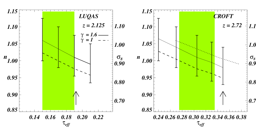
Figure 8: Left: The values of $\sigma_{8}$ and $n$ of the best fitting COBE normalized linear power spectra as a function of the assumed effective optical depth, for the linear power spectrum inferred from LUQAS at $z=2.125$. The solid curve is obtained with numerical simulations with $\gamma\approx 1.6$ while the dashed curve is for simulations which were rescaled to have a density temperature relation with $\gamma=1.0$. Shaded regions indicate our preferred values for the effective optical depth as obtained from high-resolution spectra. The arrow indicates the estimate obtained by Press, Rybicki & Schneider (1993) from low-resolution spectra. Right: The same for our re-analysis of the Croft et al. (2002) data at $z=2.72$. The dotted line in the right panel is the lower redshift result scaled by a factor 0.305/0.17 in the $x$-axis.

5.4 Combining CMB and Lyman-$\alpha$ forest data to constrain $n$ and $\sigma_{8}$

The measurement of the amplitude of the matter power spectrum on scales of a few Mpc with the Lyman-$\alpha$ forest is a powerful tool to constrain the spectral index of primordial density fluctuations when combined with measurements on large scales from CMB fluctuations (see Phillips et al. 2001 for a detailed discussion). The linear matter power spectrum at $z=0$ can be written as,

$$P_{\rm mat}(k)=A\,k^{n}\,T^{2}(k),$$ (8)

where $T(k)$ is the matter transfer function which depends on cosmological parameters in the usual way.

To get a first idea how the spectral index inferred by such a combined analysis depends on $\tau_{\rm eff}$, we here assume a COBE normalized power spectrum and no contribution by tensor fluctuations. We then find the best fitting spectral index $n$ (having fixed the other cosmological parameters to our fiducial values). We use CMBFAST to calculate the theoretical linear power spectra (Seljak & Zaldarriaga 1996). Note that normalizing to the WMAP data would give similar results. The thick solid curve in Figure 8 shows the result for a range of $\tau_{\rm eff}$ using numerical simulations which have $\gamma\approx 1.6$ and $T_{0}\approx 10^{4.15}$ K. The left and right panel are again for the LUQAS and C02 sample, respectively. The shaded regions indicate the range of $\tau_{\rm eff}$ preferred by high-resolution absorption spectra as discussed in Section 2.4. For the errors we have added the statistical errors and the systematic errors in Table 5 in quadrature. Note that in Figure 8 we have omitted the error due to $\tau_{\rm eff}$ and $\gamma$ as the dependence on these parameters is shown explicitely.

Once the spectral shape and the cosmological parameters are fixed, the measurement of the fluctuation amplitude on Lyman-$\alpha$ forest scales can also be expressed in terms of $\sigma_{8}$, the rms fluctuation amplitude of the density for a 8 $h^{-1}$ Mpc  sphere. The corresponding values are shown on the right axis of Figure 8. Note that the scale corresponding to 8 $h^{-1}$ Mpc  is $\sim 0.008\,{\rm s/km}$ at $z=2.72$ (assuming again the cosmological parameters of Section 3). The flux power spectrum is thus a direct probe of $\sigma_{8}$ for the range of $k$-values used in our analysis.

The inferred values of $\sigma_{8}$ and $n$ will also depend on the assumed cosmological parameters (see Phillips et al. 2001 for a detailed discussion). Most important is the dependence on $\Omega_{\rm 0m}$ and $h$. For a flat cosmological model, the spectral index scales approximately as $n\propto(\Omega_{\rm 0m}h^{2})^{-0.35}$ (Phillips et al. 2001). In Figure 9, we show the depencence of the inferred value of $\sigma_{8}$ on $\Omega_{\rm 0m}$ for a flat universe. This dependence is essentially negligible. The dependence on $h$ is also weak. For the error estimate we have added all values in Table 5 in quadrature. Table 6 lists our final estimate of $\sigma_{8}$ and $n$ for the LUQAS and C02 sample, as well as their weighted mean.

Table 6: Estimated values of $\sigma_{8}$ and $n$ and their errors ($\gamma=1.3$ and $\tau_{\rm eff}=0.17$ and $\tau_{\rm eff}=0.305$ at $z=2.125$ and at $z=2.72$. Note that $n$ scales as $n\propto(\Omega_{\rm 0m}h^{2}/0.135)^{-0.35}$ ^(a).

	LUQAS	C02	combined
$\sigma_{8}$	$0.95\pm 0.04{(\rm stat.)}\pm 0.13{(\rm syst.)}$	$0.92\pm 0.04{(\rm stat.)}\pm 0.13{(\rm syst.)}$	$0.93\pm 0.03{(\rm stat.)}\pm 0.09{(\rm syst.)}$
$n$	$1.02\pm 0.02{(\rm stat.)}\pm 0.08{(\rm syst.)}$	$0.99\pm 0.02{(\rm stat.)}\pm 0.08{(\rm syst.)}$	$1.01\pm 0.02{(\rm stat.)}\pm 0.06{(\rm syst.)}$

• Note that there is an additional uncertainty in the COBE normalization (Bunn & White 1997).

Figure 9: The value of $\sigma_{8}$ of the best fitting COBE normalized linear power spectra as a function of the assumed $\Omega_{\rm 0m}$ for the linear power spectrum, inferred from LUQAS at $z=2.125$, and from the C02 data at $z=2.72$. The assumed effective optical depths are $\tau_{\rm eff}=0.17$ and $\tau_{\rm eff}=0.305$ and the exponent of the temperature-density relations was $\gamma=1.3$.

5.5 Gravitational growth

Our subsample drawn from the LUQAS sample was chosen to maximise the contrast in redshift with respect to the C02 sample, and to further investigate the redshift evolution of the flux power spectrum. There are two effects which are responsible for the evolution of the flux power spectrum, the decrease of $\tau_{\rm eff}$ with decreasing redshift, and the increase of the fluctuation amplitude of the matter power spectrum due to gravitational growth. As can be seen by comparing the right and left panels of Figure 5, the net effect is a decrease of the flux power with decreasing redshift which is, however, significantly smaller than that expected from the decrease of $\tau_{\rm eff}$.

In order to assess if the flux power spectra of the LUQAS and C02 samples are consistent with the expected gravitational growth of the matter power spectrum between the two redshifts, we can compare the inferred values of $\sigma_{8}$, which should then be the same. To facilitate such a comparison, the dashed curve in the right panel of Figure 8 is the inferred $\sigma_{8}$ of the LUQAS sample (shown in the left panel) with all effective optical depths scaled by the same factor of $0.305/0.17$. The inferred values of $\sigma_{8}$ agree to within the errors, and the evolution of the flux power spectrum between $z=2.7$ and $z=2.1$ is fully consistent with being due to the expected gravitational growth and the observed evolution of $\tau_{\rm eff}$. The same was found by C02 when they compared their fiducial sample to their low-redshift subsample.

6 Discussion and Conclusions

We have used the observed flux power spectrum of two large samples of high-resolution spectra, a sample drawn from LUQAS at a median redshift of $z=2.125$, and the sample compiled by Croft et al. (2002) at $z=2.72$, together with a suite of high-resolution numerical simulations, to infer the dark matter power spectrum on scales $0.003<k$(s/km)$<0.03$.

We have obtained the following results:

1. With the same assumptions for effective optical depth, density-temperature relation, and cosmology, our inferred linear matter power spectrum agrees very well with that inferred by Croft et al. (2002).

2. We confirm previous results that the inferred rms amplitude of density fluctuations depends strongly on the assumed $\tau_{\rm eff}$. It increases by 20% if we assume an optical depth of $\tau_{\rm eff}=0.305$ a value suggested by studies of high-resolution absorption spectra. We find, however, a dependence on $\tau_{\rm eff}$ which is weaker than that of C02 and stronger than that of GH02.

3. For values $\tau_{\rm eff}$ suggested by high-resolution absorption spectra the linear power spectrum of the best fitting running spectral index model of Spergel et al. (2003) falls significantly below the linear power spectrum inferred from both the LUQAS and the C02 sample.

4. The decrease of the amplitude of the flux power spectrum between $z=2.7$ and $z=2.1$ is consistent with that expected due to the decrease of $\tau_{\rm eff}$ and the increase of the amplitude of matter power spectrum due to gravitational growth.

5. Our estimate of the systematic uncertainty of the rms fluctuation amplitude of the density ($\sim 14.5\%$) is a factor 3.5 larger than our estimate of the statistical error ($\sim 4\%$). The systematic uncertainty is dominated by the uncertainty in the mean effective optical depth and — somewhat surprisingly — by the uncertainties between the numerical simulations of different authors. Reducing the overall errors will thus mainly rely on a better understanding of a range of systematic uncertainties.

6. By combining the CMB constraint (assuming that there is no contribution from tensor fluctuations) on the amplitude of the DM power spectrum on large scale with the high-resolution Lyman-$\alpha$ forest data we obtain $n=1.01\;(\Omega_{\rm 0m}h^{2}/0.135)^{-0.35}\;\pm 0.02{(\rm statistical)}\pm 0.06{(\rm systematic)}$ for the spectral index. The corresponding rms fluctuation amplitude is, $\sigma_{8}=0.93\pm 0.03{(\rm statistical)}\pm 0.09{(\rm systematic)}.$

References

- [] Adelberger K. L., Steidel C. C., Shapley A. E., Pettini M., 2003, ApJ, 584, 45
- [] Bernardi M., et al., 2003, AJ, 125, 32
- [] Bennett C. L., et al., 2003, ApJS, 148, 1
- [] Bruscoli M., et al., 2003, MNRAS, 343, 51
- [] Bunn E. F., White M., 1997, ApJ, 480, 6
- [] Choudhury T.R., Srianand R., Padmanabhan T., 2001, ApJ, 559, 29
- [] Croft R. A. C., 2003, astro-ph/0310890
- [] Croft R. A. C., Weinberg D. H., Katz N., Hernquist L., 1998, ApJ, 495, 44
- [] Croft R. A. C., Weinberg D. H., Pettini M., Hernquist L., Katz N., 1999b, ApJ, 520, 1 (C99)
- [] Croft R. A. C., Weinberg D. H., Bolte M., Burles S., Hernquist L., Katz N., Kirkman D., Tytler D., 2002, ApJ, 581, 20 (C02)
- [] Desjacques V., Nusser A., Haehnelt M. G., Stoehr F., 2004, MNRAS, in press
- [] Eisenstein D. J., Hu W., 1999, ApJ, 511, 5
- [] Gnedin N. Y., Hui L., 1998, MNRAS, 296, 44
- [] Gnedin N. Y., Hamilton A. J. S., 2002, MNRAS, 334, 107
- [] Hui L., 1999, ApJ, 516, 519
- [] Hui L., Gnedin N., 1997, MNRAS, 292, 27
- [] Hui L., Burles S., Seljak U., Rutledge R. E., Magnier E., Tytler D., 2001, ApJ, 552, 15
- [] Kim, T.-S., Carswell, R. F., Cristiani, S., D’Odorico, S., Giallongo, E. 2002, MNRAS, 335, 555
- [] Kim, T.-S., Viel M., Haehnelt M.G., Carswell R.F., Cristiani S., 2004, MNRAS, 347, 355 (K04)
- [] McDonald P., Miralda-Escudé J., Rauch M., Sargent W.L., Barlow T.A., Cen R., Ostriker J.P., 2000, ApJ, 543, 1 (M00)
- [] McDonald P., 2003, ApJ, 585, 34
- [] Meiksin A., White M., 2001, MNRAS, 324, 141
- [] Meiksin A., White M., 2003, astro-ph/0307289
- [] Press W. H., Rybicki G. B., Schneider D. P., 1993, ApJ, 414, 64
- [] Phillips J., Weinberg D. H, Croft R.A.C., Hernquist L., Katz N., Pettini M., 2001, 560, 15
- [] Rauch M., 1998, ARA&A, 36, 267
- [] Ricotti M., Gnedin N., Shull M., 2000, ApJ, 534, 41
- [] Schaye J., Theuns T., Rauch M., Efstathiou G., Sargent W. L. W., 2000, MNRAS, 318, 817
- [] Schaye J., Aguirre A., Kim T.-S., Theuns T., Rauch M., Sargent W. L. W., 2003, ApJ, 596, 768
- [] Seljak U., Zaldarriaga M., 1996, ApJ, 469, 437
- [] Seljak U., McDonald P., Makarov A., 2003, astro-ph/0302571
- [] Spergel D. N. et al. 2003, ApJS, 148, 175
- [] Springel V., Yoshida N., White S. D. M., 2001, NewA, 6, 79
- [] Springel V., Hernquist L., 2002, MNRAS, 333, 649
- [] Springel V., Hernquist L., 2003, MNRAS, 339, 289
- [] Theuns T., et al., 1998, MNRAS, 301, 478
- [] Theuns T., Viel M., Kay S., Schaye J., Carswell B., Tzanavaris P., 2002, ApJ, 578, L5
- [] Tytler D., et al., 2004, astro-ph/0403688
- [] Verde L., et al. 2003, ApJS, 148, 195
- [] Viel M., Matarrese S., Theuns T., Munshi D., Wang Y., 2003, MNRAS, 340, L47
- [] Viel M., Haehnelt M. G., Carswell R. F., Kim T.-S., 2004a, MNRAS, 349, L33
- [] Viel M., Matarrese S., Heavens A., Haehnelt M. G., Kim T.-S., Springel V., Hernquist L., 2004b, MNRAS, 347, L26
- [] Weinberg D., 1999, in: Evolution of large scale structure : from recombination to Garching, eds. A. J. Banday, R. K. Sheth, L. N. da Costa., p.346
- [] Weinberg D.H., Dave’ R., Katz N., Kollmeier J.A., 2003, AIP conf. Proc. 666, 157-169
- [] Zaldarriaga M., Hui L., Tegmark M., 2001, ApJ, 557, 519
- [] Zaldarriaga M., Scoccimarro R., Hui L., 2003, ApJ, 590, 1
- [] Zuo L., Bond J. R., 1994, ApJ, 423, 73