Abstract
A simple and general description of the dynamics of a narrow-eccentric ring is presented. We view an eccentric ring which precesses uniformly at a slow rate as exhibiting a global mode, which can be seen as originating from a standing wave superposed on an axisymmetric background. We adopt a continuum description using the language of fluid dynamics which gives equivalent results for the secular dynamics of thin rings as the the well known description in terms of a set of discrete elliptical streamlines formulated by Goldreich and Tremaine (1979). We use this to discuss the non linear mode interactions that appear in the ring through the excitation of higher modes because of the coupling of the mode with an external satellite potential, showing that they can lead to the excitation of the mode through a feedback process. In addition to the external perturbations by neighboring satellites, our model includes effects due to inelastic inter-particle collisions. Two main conditions for the ring to be able to maintain a steady normal mode are obtained. One can be expressed as an integral condition for the normal mode pattern to precess uniformly, which requires the correct balance between the differential precession induced by the oblateness of the central planet, self-gravity and collisional effects is the continuum form of that obtained from the streamline model of Goldreich and Tremaine (1979). The other condition, not before examined in detail, is for the steady maintenance of the non-zero radial action that the ring contains because of its finite normal mode. This requires a balance between injection due to eccentric resonances arising from external satellites and additional collisional damping associated with the presence of the mode. We estimate that such a balance can occur in the ring of Uranus, given its currently observed physical and orbital parameters.
Structuring eccentric-narrow planetary rings
J.C.B. Papaloizou and M.D. Melita
Astronomy Unit.
School of Mathematical Sciences.
Queen Mary. University of London.
Mile End Rd.
London E1 4NS. U.K.
49 pages, 1 Figure
Proposed Running Head: Structuring eccentric-narrow planetary rings
Editorial correspondence to:
J.C.B. Papaloizou
Astronomy Unit.
School of Mathematical Sciences.
Queen Mary. University of London.
Mile End Rd.
London E1 4NS. U.K.
Telephone +44 (0)20 7882 5446
Fax +44 (0)20 8983 3522
email: jcbp@maths.qmul.ac.uk
Keywords: Planetary rings, Celestial Mechanics
1 Introduction
The nature of the dynamical mechanism that maintains the apse alignment of narrow-eccentric planetary rings is one of the most interesting and challenging problems of Celestial Mechanics.
According to the leading model (Goldreich and Tremaine 1979) the self-gravity of the ring counter-acts the differential precession induced by the oblateness of the central planet. Using this hypothesis, a prediction of the total mass of the ring can be made, which, in general, is not in good agreement with the inferred mass of the observed eccentric rings in the Uranus system (Tyler et al. 1986, Graps et al. 1995, Goldreich and Porco 1987, Porco and Goldreich 1987). This led to the consideration of other factors that might play an important role in the dynamics. In particular, at their narrowest point, the ring particles are ‘close-packed’. In such a situation particle interaction or pressure effects may affect the precession of particle orbits. A simple model where the pinch locks the differential precession, was introduced by Dermott and Murray (1980). A more global picture, including the effect of stresses due to particle interactions and neighboring satellite perturbations, which offered a better agreement with the observations, has been produced by Borderies et al. (1983). Their dynamical model is described in terms of mutually interacting streamlines and the satellite interactions (see Goldreich and Tremaine 1981) are computed using a resonance-continuum approximation. The standard self-gravity model was later revisited by Chiang and Goldreich (2000), who considered the effects of collisions near the edges, proposing that a sharp increase of an order of magnitude in the surface density should be observed within the last few hundred meters of the ring edges. More recently, employing a pressure term that describes close-packing, Mosqueira and Estrada (2002) obtained surface-density solutions that agree well with the currently available mass estimates.
However, several questions remain, such as how steady global modes are maintained by intercations with a satellite and mode couplings against dissipative processes. In particular if such modes are associated with particle close packing at certain orbital phases, this is likely to produce enhanced dissipation that has to be made up through the action of satellite torques. Here we consider the issue as to how the torque rate input available from satellites can counteract such collisional dissipation.
In this work we build, from first principles, a simple general continuum or fluid like model of a narrow-eccentric ring. The eccentric pattern in the ring can be described as being generated by a normal mode of oscillation of wave-number which may be considered to be a standing wave. Dissipation can be allowed to occur due to inter-particle collisions leading to a viscosity which would lead to damping of the mode. However, this global mode can also be perturbed by neighboring-shepherd satellites which can inject energy and angular momentum through resonances. In this way losses due to particle collisions may be balanced. It is that process that is the focus of this paper. Other possible mechanisms, such as mode excitation through self-excitation through viscous overstability, that could arise with an appropriate dependence of viscosity on physical state variables (see Papaloizou and Lin 1988, Longaretti & Rappaport 1995), are beyond the scope of this paper and accordingly not investigated here.
To describe the ring perturbations and the mode we use the Lagrangian-displacement of the particle orbits from their unperturbed circular ones (for a similar treatment applied to very diverse problems see for example Lebovitz 1967, Lynden-Bell and Ostriker 1967, Friedman and Schutz 1978, Shu et al. 1985).
In section 2 we set up the equations for the Lagrangian variations starting from the equations of motion in a 2D flat disk approximation. We also compute the Lagrangian variation of the satellite potential as seen by a particle as a consequence of the existence of the mode, and we discuss what non linear couplings appear in the ring as a result including the excitation of the mode through a feedback process. In section 3 we derive the radial equation of motion for the 2D Lagrangian displacement under the assumption that the ring is primarily in a normal mode. The definition of the radial action in terms of the Lagrangian displacement for small eccentricities is given in section 4, and its rate of change is obtained. We can then determine a condition for the steady maintenance of the amplitude or eccentricity associated with the mode, which requires the external satellite input to balance the dissipative effects due to collisions.
In this paper, the application we consider is to the ring of Uranus. As there are no effective corotation resonances in this ring if the eccentricity of the perturbing satellites is neglected as is done here, we shall consider only Lindblad resonances and defer consideration of corotation resonances to future work.
The satellite torque is obtained in section 5. In section 6 we show that for the narrow rings considered here, the satellite contribution to the rate of change of the radial action is just a fraction of the corresponding satellite torque dependent only on the relevant azimuthal mode number,
The additional condition for the existence of the normal mode, i.e. the condition of uniform-precession, is derived in section 7. The self-gravity term appearing in this condition is computed in section 8. In section 9 we show that the eccentricity gradient is necessarily positive in a narrow-ring which in which uniform precession is mainly maintained by self-gravity and we estimate its value in the linear regime.
In section 10 we discuss our results and by considering the total ring radial action using a very simple N-body approach, we illustrate the global functioning of a narrow-eccentric ring. We are able to obtain both ring spreading and the balance of satellite torques and collisional dissipation required to maintain ring eccentricity in various limiting cases of ring evolution. Finally, we apply our results to the ring of Uranus estimating that the balance between the satellite torque input and the dissipative effects necessary to maintain its eccentricity can be established in this case.
2 Equations of Motion and Lagrangian Displacement
We adopt a continuum or fluid description of the system from a Lagrangian viewpoint. There is an issue about whether such a description is applicable to planetary rings for which the particle collision time is typically comparable to the orbital time. An approach based on taking moments of the Boltzmann equation (see Stewart, Lin and Bodenheimer 1984 for a discussion) yields fluid equations with a stress tensor that is determined by the details of the collisional behavior and therefore uncertain. However, this consideration only affects viscous and pressure effects. Phenomena such as density waves which control global modes are independent of it (see Shu 1984 for more discussion). Furthermore some viscous phenomena like those considered here are related to conservation laws so that the way they enter is clear even if details are uncertain. A Lagrangian description is the natural one because the description of Keplerian orbits is straightforward and in a ring for which particle motion deviates slightly from Keplerian, torques due to satellites acting on the ring etc. arise from changes as seen by a moving fluid element.
Goldreich and Tremaine (1981) and Borderies, Goldreich and Tremaine (1983) adopt an approach in which ring particles are assumed to be on elliptical streamlines with slowly varying (compared to orbital times) osculating Keplerian elements. In many ways that approach and the one followed here are similar.
But the assumption of slow variation means that disturbances producing satellite torques are not included directly as they need to be for mode coupling. Also this model is a discrete one consisting of streamlines. This necessitates care with regard to the singular integrals, that need to be taken in the principal value sense, that occur when dealing with self-gravity (see section 8 below ).
We start from the basic equations of motion for a particle in Lagrangian form in 2D:
| (1) |
| (2) |
Here define the cylindrical coordinates of the particle referred to an origin at the center of mass of the planet. Here denotes the gravitational potential due to both the central planet, the neighboring satellites and the ring. In addition denote the radial and azimuthal components of any additional force per unit mass respectively. This may arise through internal interactions between particles that might lead to an effective pressure and/or viscosity. However, we do not need to introduce such concepts in order to derive our condition determining the growth or decay of global modes.
We introduce a Lagrangian description in which the system is supposed to be perturbed from an axisymmetric state in which particles are in circular motion with coordinates such that Here is the fixed radius of the particle concerned, is the angular velocity and is a phase factor labeling each particle. In keeping with a Lagrangian description are conserved quantities for a particular particle and so may be used to label it.
In order to describe the system when it is perturbed from the axisymmetric state we introduce the components of the Lagrangian displacement These are such that the coordinates of each particle satisfy:
| (3) |
and
| (4) |
To obtain equations for and we take variations of Eq.’s (1) and (2). We do this by applying the Lagrangian difference operator, , as defined by Lebovitz (1961) to both sides of Eq.’s (1) and (2). For a given quantity , the variation is defined by:
| (5) |
where and are the values of the given physical quantity in the perturbed and unperturbed flow respectively. In contrast, the Eulerian difference operator is defined as:
| (6) |
Thus, to first order in they are related through:
| (7) |
which gives the linear form of the Lagrangian difference operator.
2.1 Equations for the Lagrangian displacement
Following Shu et al. (1985) we assume that the components of the displacement are small enough that they can be treated as linear in the sense that On the other hand the radial gradient of the radial displacement may be large so that may be of order unity. The significance of these assumptions is that although the ring eccentricity is assumed to be everywhere small, the ring surface density perturbation induced by it may be of order unity. Adopting them enables us to perform the variation in the accelerations using the linear form of the difference operator as described above, wherever radial gradients are not involved. These then satisfy:
| (8) |
| (9) |
Here the potential due to the satellites, , and that due to the self-gravity of the ring, , are included in Thus The quantities denote the variational components of the force per unit mass due to particle interactions which can include viscous effects. In this paper we do not need to make explicit use of these apart from their production of an impulsive interaction (see section 10.2 ) so they will be left unspecified. The full non linear Lagrangian variation is retained for and as these may involve the density variation. Contributions coming from the variation of the central planet potential are included on the left hand side of Eq. (8).
2.1.1 Replacement of convective derivatives
Lynden-Bell and Ostriker (1967) showed that to first order in the perturbations, the operator and the convective operator commute. But note that the fact that the time derivative is taken at constant taken together with the definition (5) means that this is true in general. Thus for a given quantity we have:
| (10) |
For quantities not involving radial gradients we may linearize and thus use the unperturbed velocity field in working out the convective derivative. We can then write:
| (11) |
where:
| (12) |
Thus, dropping the subscript, we can write the convective derivative following the unperturbed motion, and for any quantity is:
| (13) |
Similarly
| (14) |
2.2 Surface density perturbation and Lagrangian variation of the satellite potential
We suppose the ring particles to be in eccentric orbits and combine to form a globally eccentric ring. This is described using a surface density distribution and eccentricity distribution We also consider there to be an axisymmetric reference state for which and from which we can regard the eccentric ring as being the result of a perturbation. The perturbation of the surface density is of the form:
| (15) |
For linear perturbations where the azimuthal mode number, The eccentric ring can be thought of as being primarily in a mode with azimuthal mode number In practice we may assume
In addition we suppose the ring to be perturbed by a satellite which produces a contribution to of the form:
| (16) |
for general with being the satellite’s orbital frequency.
Note that the analysis presented below may be generalized to include more than one such term by linear superposition. Expressing the gradients of in cylindrical coordinates, , gives:
| (17) |
and
| (18) |
where we denote Note too that we include the components of the gradient of the satellite potential prior to application of the displacement as the first terms in (17) and (18). This is because these were not included in the treatment of the unperturbed axisymmetric ring.
2.3 Displacements and couplings in the ring
Associated with each azimuthal mode number is a displacement Such a displacement is excited by the direct action of the satellite acting through the first terms in Eq.’s (17) and (18). This part of the response is that associated with a satellite in circular orbit acting on a ring in which the particles are also on circular orbits. In appendix 1 we show why this interaction does not lead to the development of eccentricity in the ring.
In addition, when it is present, the eccentric mode provides an independent displacement in the ring with In a treatment that is fully linearized in all displacements and exciting potentials this could be superposed with that excited directly by the satellite.
However, at an order which is the product of the displacement and the satellite potential effective forcing arising from terms depending on the product of the displacement component with and gradients of in Eq.’s (17) and (18) generates displacement responses with azimuthal mode numbers and One or both of these may produce a resonant response and be important for the dynamics. This is because such a resonant response can recouple back through the potential to excite the original mode resulting in a feedback process,
Here, we focus on the component with and its associated displacement However, the component with may be considered by linear superposition if that is important. Thus, with a single subscript denoting the azimuthal mode number, we consider a general displacement of the form:
| (19) |
The first term represents the displacement associated with mode in the ring that accounts for the observed eccentricity. The second term is the displacement directly excited by the circular orbit satellite forcing potential and the third term is the displacement excited through the coupling of the satellite potential to the displacement.
3 The m=1 (eccentric) mode
We here consider the mode which causes the ring to be eccentric. In the inertial frame the pattern associated with this mode rotates at a low frequency, characteristic of the orbital precession frequency and the natural time scale of variation is Thus:
| (20) |
Recalling that the left hand side of Eq. (9) approximated by the linearized form, gives for the azimuthal component of the displacement:
| (21) |
where the quantity is defined by:
| (22) |
Using (20) gives the adequate approximation:
| (23) |
Firstly we comment that linear perturbations are strictly separable. In that approximation, the component of the displacement satisfies (Shu et al. 1985):
| (24) |
Secondly we comment that the motion is dominated by the force due to the central mass, and to within an error governed by the magnitude of the other forces acting in comparison, is Keplerian. This means that to within this limit which is also measured by the ratio of orbital precession frequency to orbital frequency
| (25) |
which applies to Keplerian orbits with small eccentricity.
Furthermore (21) tells us that the magnitude of compared to that of is of order the ratio of forces producing non Kepler motion to the force due to the central mass.
Using (21) and the assumption of slow rate of change to neglect second partial derivatives with respect to time in Eq. (8) one then finds that the component of the displacement satisfies:
| (26) |
Here the square of the epicyclic frequency is given by:
| (27) |
To evaluate the Lagrangian change to the gradient of the satellite potential we insert Eq. (19) in Eq. (17). However, we retain only the terms with azimuthal dependence corresponding to The assumption here is that only these produce significant secular effects on the mode. Other terms produce small corrections with a different and in general much more rapidly varying azimuthal dependence.
Thus we adopt the following combination of terms from (17):
| (28) |
where refers to terms that can contribute secularly to the mode. Note that because has azimuthal mode number it is not included. Notice that the retained terms are the only non-vanishing ones when multiplied by and integrated over
4 Conservation of radial action
As is well known, the radial action, taken here to be per unit mass associated with a Keplerian orbit around the central mass, here being the semi-major axis is an adiabatic invariant. As the ring particles are always close to eccentric Keplerian orbits, we might expect to find a related quantity.
To do this we define:
| (29) |
Here and in other similar integrals are taken over the entire radial and azimuthal domain of the ring.
To see that for displacements the above integral corresponds to the radial action we note that if we identify and use the fact that:
| (30) |
may be written:
| (31) |
with being a mass element associated with the ring. This corresponds to a multiple of the standard radial action expanded to first order in
4.1 Rate of change of radial action for the ring
We first comment that self-gravity makes no contribution (see appendix 2 for details) and so when calculating the rate of change of radial action in this section we may replace by
By multiplying (26) by and integrating over the mass of the ring we obtain an expression for the time rate of change of the radial action in the form:
| (32) |
We do an integration by parts with respect to making use of (23) together with (18) This procedure enables us to eliminate in terms of the satellite potential. Then (32) becomes:
| (33) |
Eq. (33) gives a conservation law for the radial action associated with the mode.
In the absence of collisional terms involving and terms involving the satellite potential, as expected the radial action is conserved. It is important to note that the collisional terms act on the perturbation from an axisymmetric state and are not necessarily negative definite leading to a decay of the radial action ( see eg. Papaloizou and Lin 1988 ) though in general one might expect that to be the case. The terms on the right hand side of (33) that depend on the m-component of the satellite potential can also change the radial action when the satellite forcing leads to secular changes due to waves launched at resonance (see eg. Goldreich and Tremaine 1980).
For a ring in which a steady eccentricity is maintained the secular rates of change due to satellite forcing must balance those due to the effects of viscosity or collisions acting on the perturbations. In such a case we have a condition such that remains constant.
Notice that there is no net-contribution from self-gravity when integrated over the mass of the ring, hence, any dissipation arising from internal friction can only be compensated by external forces, i.e. the satellite torques (see also the discussion below). The exact fraction of the satellite torque that acts on the ring so as to maintain the mode is calculated in the next section.
5 The satellite Torque
The satellite potential terms arising on the right-hand side of Eq. (33) are directly related to the resonant torque generated by the forcing between satellite and ring as occurs in Eq.’s (8) and (9) through the forcing gradient of potential components:
| (34) |
and
| (35) |
where the terms not containing the components are ignored thus the unsubscripted displacement is the component. Note that the forcing amplitude is proportional to both the satellite potential and the ring eccentricity. Note that in principle additional forcing terms can arise from the components of with azimuthal mode number Such components can for example be generated from terms proportional to the ring eccentricity and those coming from the response to the satellite forcing potential component with azimuthal mode number However, this response is non-resonant in the neighborhood of the Lindblad resonance where the response to forcing is located. Forcing terms of this type are not considered here as they arise from forces internally generated in the ring, which are assumed small compared to those arising from direct forcing. Furthermore we only require the ring-satellite torque produced by the direct forcing of the unperturbed background ring through Eq.s (34) and (35) which from the above discussion should represent almost the total torque.
The total torque can be estimated as in Goldreich and Tremaine (1978). To provide an expression for this torque, we return to the equations of motion (8) and (9). From these the rate of change of ring canonical energy (see Freidman and Schutz 1978) associated with the response with azimuthal mode number is obtained as the rate of doing work as a result of the forcing as:
| (36) |
We now use the fact that because the disk is forced by a disturbance with a definite pattern speed, say the rate of change of ring angular momentum is given by:
| (37) |
which expresses the well known result that the ratio of energy to angular momentum exchanged is (see also Freidman and Schutz 1978).
Similarly for the perturbation itself we have:
| (38) |
6 The Radial action and the satellite Torque
We write the satellite potential as in Eq. (16) and the displacements as:
Where is the slow pattern frequency or precession frequency associated with the mode as seen in the inertial frame. is the azimuthal phase shift undergone by the wave crests between the resonance location and (see for example Goldreich and Tremaine 1978). Notice that for the mode this is a very small quantity that has been neglected. The amplitude of the mode, , is a function of the satellite forcing.
We also assume that the disturbance is generated and significant only near a Lindblad resonance. For the case with azimuthal mode number this is where:
We note that the pattern speed is and the necessary choice of negative sign, to enable the resonance to lie within the ring means that it corresponds to an outer Lindblad resonance. This occurs where the ring rotates more slowly that the satellite and, accordingly, gains angular momentum.
Were we dealing with the case of azimuthal mode number the choice of positive sign would be necessary and we would have an inner Lindblad resonance at which the ring lost angular momentum.
To within an error of order the ratio of the precession to orbital frequency (typically for the ring around Uranus; see section 10) we may replace by and use the relation between and that applies at and in the neighborhood of a Lindblad resonance. To determine this relation, internal forces arising in the ring and from any satellite may be neglected. Eq. (9) then reduces to:
| (41) |
Using Eq. (13) together with Eq. (38) we find:
| (42) |
Because we are close to resonance, we use the above condition for an outer Lindblad resonance to get so obtaining:
| (43) |
This is very similar to Eq. (25) which reads
| (44) |
From (43) and (44) we find the useful result that
| (45) |
Then, the non vanishing terms in Eq. (40) lead to:
| (46) |
The above coefficients are given by:
| (47) |
It turns out that the terms associated with the satellite-potential which ultimately give a non vanishing contribution in Eq. (33) which gives the rate of change of ring radial action can be expressed as multiple of Eq. (46). Thus:
where the subscript here denotes an azimuthal average and it is verified that:
Thus, Eq. (33) can be re-written as:
We can also add in the effects of forcing with azimuthal mode number should that lead to secular effects by replacing by
Note that the absolute value of appears as the case of azimuthal mode number corresponds to an inner Lindblad resonance for which
We may then write Eq. (33) in the compact form applicable to a thin ring:
| (48) |
Here may be evaluated at the ring center and:
| (49) |
is a quantity having the dimensions of the rate of energy dissipation of the perturbed motion. Eq. (48) gives a condition for non zero radial action to remain constant, that requires external satellite torque input to balance dissipative effects due to particle collisions.
We comment here in the context of an application below (see section 10) that the dissipative term takes a particularly simple form when the forces per unit mass are taken to produce small impulsive changes in the perturbed motion that may for example take place once per orbit at pericenter (see Eqs. 8 and 9). Then
| (50) |
which is the difference in kinetic energy before and after the impulse as experienced by a fluid element as evaluated using the Lagrangian velocity perturbations per orbital period.
However, as is well known there is another condition that has to be satisfied in order that the ring may possess a steady mode. This comes about because the ring has to precess at a uniform rate. This requires internal forces due to self-gravity and particle collisions to balance the differential precession that would occur if ring particles moved freely under the central potential (see for example Chiang and Goldreich 200). We now give an expression for this condition in a similar format to that of Eq. (48).
7 The condition for uniform precession
The mode responsible for the ring eccentricity has a constant and very small pattern speed as viewed in the inertial frame. This means that individual ring particles appear to be in elliptic orbits that precess at the same rate. In oder to achieve this the internal and external forces acting in the mode have to satisfy a constraint that can be view as a non-linear dispersion relation. Our treatment again follows that of Shu et al. (1985) who provided such a relationship for density waves in Saturn’s rings. Except here we consider a density wave comprising a global normal mode rather than a forced propagating wave.
Eq. (8) can be expressed in the form:
| (51) |
We now use an angle that is fixed with respect to a coordinate system rotating at the pattern angular frequency namely The radial displacement is taken to be of the form Following Shu et al. (1985) we note that as the time dependence is contained within only depends on and
Multiplying Eq. (51) by and integrating over we obtain:
| (52) |
where:
| (53) |
and
| (54) |
We note here that the satellite potential does not contribute to the determination of the mode to within an error on the order of the ratio of the satellite forcing potential to that due to the central mass and so is neglected in this section.
The last term in Eq. (52) can be re-written after an integration by parts as in section 4 in the form:
| (55) |
where:
| (56) |
Here we have assumed that the azimuthal scale is much longer than the radial one so that the azimuthal component of the acceleration due to self-gravity can be neglected in comparison to the radial one (tight winding approximation).
Eq. (52) then becomes:
| (57) |
where:
| (58) |
Given that , where is the local radius dependent precession frequency and assuming that and , Eq. (57) can be approximated to first order in and as:
| (59) |
Eq. (59) provides a condition to be satisfied by the normal mode amplitude that can be thought of as a condition for uniform precession. It is satisfied when the self gravity, satellite forcing and the internal collisional terms represented on the right-hand side of Eq. (59) balance the differential precession term on the left-hand side. Note further that for a thin ring of the type considered here, may be taken as constant in (59) and evaluated at the ring center from now on.
8 The self-gravity term
In order to calculate we follow Shu (1985). As radial variations are much more rapid than azimuthal ones, the local self-gravity at is canonically approximated to be that due to an infinite plane sheet of radial width , where and are the inner and outer bounding radii of the ring beyond which the surface density vanishes respectively. Thus:
| (60) |
where is the mean radius of the ring and is the gravitational constant.
Note that we use in the above rather than Although the difference is apparently not significant in the slender ring approximation, we use the prescription we do to ensure that gravity remains conservative under the tight winding approximation with gravitational energy
| (61) |
Because of the small mass of the ring, self-gravity is neglected in the axisymmetric background state, consistently with that Eq. (60) gives the Lagrangian variation also. Thus
| (62) |
Note that were the background axisymmetric contribution to self-gravity incorporated here it would make no difference to the subsequent analysis as it azimuthally averages to zero.
In addition, and , where and In this planar limit, we identify the ring eccentricity as Using the tight-winding approximation we have:
| (63) |
which represents conservation of mass. We then have:
| (64) |
We can re-write Eq. (64) in terms of the eccentricity gradient, :
| (65) |
Then after integrating over we obtain (see also Shu et al. 1985):
| (66) |
where:
| (67) |
and, to within a small error of order we have replaced by Notice that the integrand in Eq. (66) presents a singularity, that has to be handled in a principal value sense, which can lead to practical complications near the ring edges.
With that comment in mind we note that when Eq.(59) is combined with Eq.(66) to give a single equation, viewed as condition for uniform precession of the ring from which one can determine one has a continuum form of Eq.(14) of Goldreich and Tremaine (1979) which gives a condition for uniform precession in terms of discrete constraints on elliptical streamlines.
9 The value of q
If we assume that is constant throughout the ring, then, from Eq. (66), it can be shown that:
| (68) |
On the other hand, from Eq. (59) we can write:
| (69) |
Thus, if the collisional impulses can be neglected with respect to the self-gravity, it is verified on setting in Eq. (69) that:
| (70) |
We remark that the pattern speed, may be regarded as an eigenvalue associated with a normal mode determined by Eq. (59). By multiplying Eq. (59) by and integrating over the ring it follows that Hence if does not change sign, as in the case of interest here, must equal the local precession frequency, at some intermediate point in the ring, , i.e. .
Then, we can write:
| (71) |
which can be put as:
| (72) |
from which we obtain: . Thus, and q (since does not change sign), is necessarily positive in any ring where self-gravity is the main mechanism that maintains apse alignment (see also Goldreich and Tremaine 1979, Borderies et al. 1983).
To estimate the value of in a narrow-eccentric ring, in the linear regime where , and if we neglect all perturbations other than self-gravity, from Eq.’s (59) and (66), we can write:
| (73) |
Here gives the magnitude of the difference between the free particle precession frequencies at the ring edges. Hence:
| (74) |
Hence, the magnitude of is basically determined by the mass, size and eccentricity of the ring.
10 Application
In this paper we have presented a description of a narrow self-gravitating ring in orbit about a dominant central mass. We have considered the situation when the ring displays an eccentricity through sustaining a global non-axisymmetric mode of oscillation. Such a mode with a single pattern speed corresponds to an eccentric ring undergoing uniform solid body precession.
We have used a continuum description of the system following that of Shu et al. (1985) for density waves in Saturn’s rings rather than a description in terms of an ensemble of interacting streamlines. One can in principle include the effects of self-gravity, viscosity or particle collisions and external satellites. In the latter case we do not assume a continuous distribution of resonant interactions (eg. Borderies et al. 1983) but allow for a small number of separated resonances.
Two main conditions for the ring to be able to maintain a mode with single slow pattern speed are obtained. One can be expressed as an integral condition for the pattern or normal mode to precess at a uniform rate (Eq. (57)) that requires the correct balance between differential precession, self-gravity and collisional effects. The other condition is one for the non zero net radial action in the ring, that exists because of its finite eccentricity, to be sustained through a balance of injection due to eccentric resonances arising from external satellites and additional collisional damping associated with the presence of the mode (Eq. (49)).
10.1 The radial action, the satellite torque and the dissipation: A more simple N-body approach
The derivation we presented above based on Fourier decomposition in the azimuthal direction was rather lengthy. We here look at how the radial action changes directly in a simpler manner and connect the result to the behavior of a global mode given by Eq. (49).
If we consider the ring as consisting of particles of mass having semi-major axes and eccentricities The total radial action is:
| (75) |
In terms of the energies and angular momenta this can be written:
| (76) |
Accordingly we have:
| (77) |
with We now find it convenient to introduce a fixed semi-major axis which could correspond to the ring center and rewrite Eq. (77) in the form:
| (78) |
where and
Now we may use the conservation of total energy and angular momentum to write:
| (79) |
and
| (80) |
where and are the rate of angular momentum and energy input into the ring from external satellites and is the rate of dissipation due to inelastic collisions. The gravitational energy of the ring resulting from its own mass distribution is while, ignoring any internal degrees of freedom in ring particles, gives the total energy content of the ring.
The ring gravitational energy is
| (81) |
where and are the position vectors of masses and respectively.
Further we suppose that some of the contribution to the satellite torques arises from non eccentric Lindblad resonances of satellites in circular orbit with pattern speed For these we accordingly have (Freidman and Schutz 1978) Further we suppose, as in section 6, that the rest comes from a satellite with an eccentric Lindblad resonance with azimuthal mode number As there, the pattern speed with being the period of the satellite. For this contribution
Using these results in (80), we find:
| (82) |
Here the subscripts and signify torques associated with the satellite and the eccentric Lindblad resonance respectively. Further, here we neglect which is small in magnitude. We recall the condition for an outer Lindblad resonance used above , namely:
| (83) |
should be satisfied within the ring. This means that, provided the relative ring thickness is significantly smaller than we can replace by and have approximately Then Eq. (82) may be written:
| (84) |
It is helpful to use the fact that we are dealing with a narrow ring and accordingly expand the first term in Eq. (84) to second order in Thus we obtain:
| (85) |
Eq. (85) is the final form of the equation for the rate of change of the total radial action for the ring. Their are several interesting limiting forms.
10.1.1 Circular ring subject to internal dissipation and satellite torques
In this limit and which vanish identically when the ring eccentricity does, are zero and we have:
| (86) |
The importance of the gravitational energy term compared to the first term on the left hand side of (86) which represents the relative kinetic energy of the ring is measured by with being the mass of the ring, This parameter is typically very small, being for the ring of Uranus and so may be neglected but we shall retain it for now.
Note too that in the case of a confined ring where changes to could only occur through changes in this term would be even smaller by a factor and thus be neglected according to our approximation scheme.
Bearing this in mind, eq. (86) can be interpreted as giving an equation for the rate of spreading of the ring. Note that the last dissipation term on the right hand side always causes the ring to spread. The terms inside the summation giving the contributions of the satellite torques are always positive definite because for standard circular orbit torques angular momentum is transferred to or from the ring according as the pattern speed exceeds or is less than the angular velocity That is for and for Thus the effect of the circular orbit Lindblad torques is to oppose dissipation and to lead to confinement.
10.1.2 Steady state ring with satellite torques and dissipation
In this case the time derivatives on the left hand side of Eq. (85) are zero and we have:
| (87) |
This expresses the balance between the satellite torques and energy dissipation. When there are no circular orbit Lindblad resonances and dissipation is induced entirely by the eccentric mode we obtain a result identical to that given by Eq. (48) in section (6), namely:
| (88) |
Note too, that as in section 6 we could add the effect of another eccentric Lindblad resonance with azimuthal mode number
In this case dissipation induced by the mode is balanced by the effects of an eccentric Lindblad resonance. Such a balance should exist independently of the existence of additional circular orbit Lindblad torques and background dissipation as the discussion in section 4 indicates. This is because it is only the eccentric resonances that can drive an eccentric mode and balance the effects of dissipation induced by such a mode.
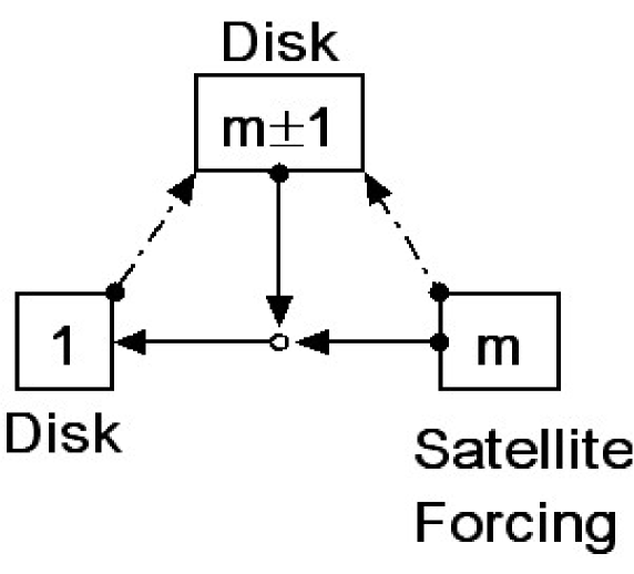
The way in which such resonances pump eccentricity has been illustrated in section 4 and it has been also discussed in the context of accretion disks in Cataclysmic binaries by Lubow (1989) and protostellar disks by Papaloizou, Nelson and Masset (2001) and Papaloizou (2002). An illustration of the interactions occurring in an eccentric ring is given in Figure 1. A short account summarizing the interaction is as follows: A potential perturbation acting on the ring with azimuthal mode number arising from a satellite in circular orbit has pattern speed This couples to the global mode producing a resonant forcing potential with azimuthal mode number The pattern speed will be This excites a resonant response at an eccentric outer Lindblad resonance. Energy and angular momentum are transferred to the ring through wave excitation. The transfer ratio is the pattern speed However, the perturbing satellite can only deliver energy and angular momentum in the ratio of its pattern speed This means that excess energy is available to be transferred into amplifying the mode which is a global disturbance rather than a resonantly excited short wavelength wave.
10.2 Application to the -ring around Uranus
We intend to show that the mechanism proposed above for the maintenance of the eccentricity in a narrow-eccentric ring can be applied to a real system. We have chosen the case of the -ring of Uranus because its orbital and physical parameters are relatively well-determined and it has known shepherd satellites.
Our goal is to verify that a reasonable estimate for the energy dissipated in the ring is of the order of the energy available from satellite torques (Eq.’s 48 and 88). Here we present a simple approach, whereas a more detailed analysis will be presented in a forthcoming paper.
We will consider only the second order resonance with Cordelia, which is the only resonance between the satellite orbit, when its eccentricity is neglected and the eccentric ring (Porco and Goldreich 1987). From Goldreich and Porco (1987) we write:
| (89) |
We shall assume that the ring is highly compressed or pinched near pericenter (Dermott and Murray 1980) to the extent that the high compression results in a an impulsive and dissipative interaction for which particle interactions and collisions are important. We comment that this situation could arise when a normal mode grows unstably to significant amplitude such that disipation becomes enhanced by non linear effects leading to limitation of the mode growth. The counterpart of this phenomenon in a fluid would be the formation of a shock. Chiang and Goldreich (2000) and Mosqueira and Estrada (2002) have considered models of the and ring in which collisional efects are important in maintaining apse alignment against the effects of differential precession induced by the planetary quadrupole moment and self-gravity. Mosqueira and Estrada (2002) explicitly consider the possibility of a pinch of the type we consider that occurs over a narrow range of azimuths near pericenter. They propose that the density reaches a limiting value there and estimate the particle dispersion velocity in order to calculate the effect of the pressure. The physical state of the ring may be complex and involve some vertical expansion ( Mosqueira and Estrada 2002). However, there may still remain a strong dissipative interaction in the pinch. Here we consider the energy balance.
The origin of the strong interaction is due to a combination of differential precession and self-gravity (cf Eq. (58).) To estimate the energy dissipated per unit mass through this strong interaction, we adopt an estimate of the relative radial kinetic energy produced by the differential precession of two orbits over one orbital period. In making this estimate we are assuming that differential precession produced by the planetary oblateness is a significant factor in the balance between that, self-gravity and collisional effects. But note that for other rings, such as the ring the balance may be between differential precession induced by self-gravity and collisional effects with both of these dominating the differential precession induced by planetary oblateness by a large factor(Chiang and Goldreich 2000, Mosqueira and Estrada 2002). In such cases, the potential collisional dissipation could be significantly underestimated by our procedure and instead the dominant differential precession rate induced by self-gravity should be adopted.
For a differential precession frequency the pericenter of two orbits will be an angle apart after one orbit. The relative radial velocity associated with epicyclic motion for this phase is Assuming that some fraction of the associated energy is dissipated every orbital period by the whole ring we obtain an estimate for the dissipation rate as
| (90) |
where is an unknown factor measuring the efficiency with which this energy is dissipated, which must satisfy: .
Using Eq. (48) we can write:
| (91) |
For the mean ring sem-major axis and surface density we adopt and respectively. For the mean ring width and eccentricity we take and respectively. The differential precession frequency between the outer and inner ring edges The mases of Uranus and Cordelia are taken to be and respectively. The azimuthal mode number associated with the resonance is
Using Eq. (48) we get for Eq. (91): . Here, in order to make simple estimates, we have used the same values of and for both sides. But we should remember that as distinct physical processes operating in different ring locations are involved, these may differ. Nonetheless this remarkable agreement shows that the eccentricity in the -ring of Uranus can be maintained due to the balance established between the satellite torque and the collisional dissipation.
However, in estimating the dissipation we only included the effects of a pinch at pericenter. We should also consider the possible magnitude of viscous dissipation arising in the general background flow. To characterize the magnitude of the kinematic viscosity we use with and being the fiducial semi-thickness associated with a monolayer with optical depth unity, having taken
The rate of disipation associated with background Keplerian flow is per unit mass (Lynden-Bell and Pringle 1974). Then
| (92) |
To compare with the above we get This is somewhat less than that estimated from the pinch effect but it could be comparable depending on the magnitude of the effective viscosity.
The background dissipation rate per unit mass produced by the eccentricity is estimated to be (see Borderies, Goldreich and Tremaine 1983). Thus this gives a rate which is factor being about a factor of five smaller than that acting from the background shear.
All of these estimates are compatible with the satellite interaction being adequate to resupply energy losses arising from both the existence of the eccentric mode and the background shear.
10.2.1 Timescales and small parameters
In view of the approximations made in the theoretical description it is of interest to compare the time scales associated with the different processes involved. The fastest time scale is the orbital timescale followed by the time scale for differential precession and the time scale for the eccentricity to decay were there to be no input from satellite torques where we took the eccentricity difference across the ring
However, if as we have postulated, the balance is between satellite torques and dissipation in the pinch, our discussion above indicates, because of the larger dissipation rate, a time scale two orders of magnitude faster of
These timescales define a small parameter being to order of magnitude the ratio of orbital time to differential precession time, enabling justification of a slow mode approximation. It is also to order of magnitude the ratio of differential precession time to eccentricity evolution time justifying a treatment of the mode neglecting in the first instance dissipative effects and apsidal twists. These can then be assumed to cause slow evolution of the mode amplitude as has been done here.
Another interesting point is that the pinch and satellite may provide the most important dissipative effects in the ring. This raises the possibility that this phenomenon also dominates the confinement process. This is a complex issue that remains to be investigated.
Appendix 1
Forcing Potentials and Ring Eccentricity Driving
We here consider the eccentricity excitation in a differentially rotating ring through the gravitational perturbation of an object in circular orbit. The issue is which terms in the forcing potential can produce eccentricity excitation. We consider a Lagrangian description. Then if fluid elements are on elliptical trajectories, an expansion of the forcing potential for a particular fluid element in powers of the eccentricity is possible.
The analysis in this paper studied the excitation of eccentricity through the ring response to the first order terms the ring eccentricity associated with a global mode, in the expansion of the satellite potential coupling back through the satellite potential itself to the global mode of the system.
The issue arises as to whether the lowest order terms in the satellite potential expansion that exist even when can participate in ring eccentricity excitation through the induced energy and angular momentum transfer they produce. We here demonstrate that such an excitation does not occur.
Form of the forcing potential
The forcing potential due to an object in circular orbit is of the form
| (93) |
Here is the orbital frequency and the pattern speed of the induced response as viewed in an inertial frame.
The energy transfer rate to the ring can be written quite generally in the form
| (94) |
with the integral being taken over the ring.
The angular momentum transfer rate may be similarly written
| (95) |
Accordingly, because of the functional dependence on and we have the general result that
| (96) |
The general idea of disk satellite interaction theory is that this transfer occurs through either the excitation of a wave at a Lindblad resonance or directly at a corotation resonance ( Goldreich and Tremaine 1981). In the situation considered here there is no corotation resonance and the transfer occurs locally as a wave is excited. At this point the wave can be regarded as propagating freely with the exciting potential playing no further role. From the above it is clear that the wave is such that its energy and angular momentum content are related by Without loss of generality we can assume that so that the interaction transfers wave energy and angular momentum to the ring.
In fact , energy and angular momentum transfer to the ring does not occur until the wave dissipates (Goldreich and Nicholson 1989). To examine how the transfer and dissipation takes place we move into the frame rotating with angular velocity in which the response appears stationary. As the forcing potential plays no further role, we can write
| (97) |
where is what would be the total Jacobi constant in the absence of dissipation and the energy dissipation rate through viscosity or collisions is From the point of view of the inertial frame, the Jacobi constant per unit mass can be written, neglecting pressure forces without loss of generality, as
| (98) |
Accordingly with and being the energy and angular momentum content of the ring. Thus as the wave dissipates
| (99) |
But from total angular momentum conservation so that
| (100) |
As angular momentum is transferred from the wave to the ring, dissipation occurs. This is because when angular momentum is transferred to local ring circular orbits with angular velocity there must at least be an associated energy transfer rate In that case this means that
| (101) |
In fact the above expression states that as the wave is completely dissipated, all the free energy associated with making the angular momentum transfer to ring material on circular orbits while maintaining them on circular orbits, which is the path that maximizes the free energy available, is dissipated by viscosity. There is accordingly none left to make the ring globally eccentric.
This situation is the expected one because although there is some free energy produced through the disk satellite interaction that takes place through the lowest order terms in the potential expansion in powers of for cases of interest, where the forcing potential has a high value of this is created in the form of a free wave with the same azimuthal mode number and is dissipated quickly and locally as described above. In such a situation, the associated radial motions being of high are not long lived and do not constitute global eccentricity. Further, in the excitation region where the forcing potential is important, they cannot couple to a global mode with very slow pattern speed( in fact their pattern speed is preserved). In order to couple to global long lived modes with slow pattern speed, terms that are first order in are required. These in turn produce torques and energy transfer rates which for small are ( see eg. Eqs. (74 - 77) of Goldreich and Tremaine 1981). In fact in this limit we would obtain the same torques in this work. The thing to remember here however, is that although produced locally, the action is transfered to a normal mode rather than an individual particle orbit.
Appendix 2
The Rate of Eccentricity Change and the Apsidal Twist
In this appendix we discuss the effects of self-gravity on the rate of change of total ring radial action and also on ring mean eccentricity. Self-gravity turns out not to enter into the expression for the time rate of change of radial action. However, it does appear in the rate of change of mean ring eccentricity provided there is a non zero apsidal twist, or the apsidal lines of the elliptical streamlines within the ring are not aligned. As the rate of change of total radial action is related to dissipation within the ring, the relation involving apsidal twist and rate of change of mean eccentricity establishes a connection between apsidal twist and dissipation.
Self-Gravity and the Rate of Change of Radial Action
Our starting point here is Eq.(26) which governs the radial component of the Lagrangian displacement:
| (102) |
In section 4.1 we obtained an equation for the rate of change of total radial action by multiplying Eq. (26) by and integrating over the mass of the ring. We here show that the forces arising from self-gravity do not contribute within the approximation scheme adopted here. In this scheme, in which the gravitational force is approximated as equivalent to that of an infinite plane sheet (see section 8 ) the acceleration due to self-gravity is taken to be non zero only in the radial direction and given by
| (103) |
Here we recall that both primed variables being functions of and unprimed variables being functions of are functions of the same angular coordinate
The potential contribution of self-gravity to the rate of change of total radial action is found from Eq. (26) to be ( see Eq. (32))
| (104) |
It is a simple matter to show after inserting (103) into (104) that the contribution to the rate of change of radial action is
| (105) |
It is straightforward by first of all noting that the integral on the right hand side is unchanged when primed and unprimed variables are interchanged and so can be replaced by half the sum of the original form and the form obtained after such an interchange. When this is done, the integrand is easily seen to be expressible as a derivative with respect to with the consequence that it integrates to zero. Thus self gravity does not contribute to the rate of change of radial action we calculate here. This result is in line with section 10.1.
Self-Gravity and the Apsidal Twist
Our starting point here is again Eq.(26). However, we now develop an equation for the rate of change of ring mean eccentricity rather than the mean square eccentricity which is connected to the radial action and which has been the theme of this paper. The equation for the time rate of change of the mean eccentricity relates this quantity to the apsidal twist of the elliptical streamlines. This twist in turn is related to the dissipation present in the ring and is accordingly expected to be very small. Accordingly it has been neglected so far.
We begin by recalling the form of displacement used above in the form and that In order to consider displacements with slowly changing eccentricity and apsidal twist we modify this to become:
| (106) |
Thus the amplitude can vary slowly with time and the twist is described by the function which could also vary slowly with time. For example the location of pericenter is given for by When varies with radius a twist is generated.
In order to proceed we insert (106) into Eq.(26) multiply by and average over the angle or equivalently or This procedure yields an expression for the evolution of the ring mean eccentricity in the form:
| (107) |
Here primed quantities denote evaluation at Working to first order in the small quantity the last integral may be written as
| (108) |
Accordingly the evolution equation for mean eccentricity is
| (109) |
Note again that the last integral again needs to be handled with caution as it is singular and requires to be interpreted in the principal value sense.
One can now obtain an expression for the rate of change of eccentricity of the entire ring by integrating over the mass. Thus
| (110) |
Here we recall that and we have made use of the symmetry properties of the second integral with respect to interchange of and
The first term on the right hand side corresponds to the effects of collisions and external satellites. We shall not dwell on this further here apart from noting that in the case of collisions the integral can be related to the total momentum change induced by them in different coordinate directions in the reference frame rotating with the eccentric pattern. As collisions conserve momentum it can be argued that the net effect is small (cf the two streamline model of Borderies, Goldreich and Tremaine 1983). Thus when external satellites are absent, there is a direct connection between apsidal twist through the second term and the rate of mean eccentricity decay. Equation (37) of the two stream model of Borderies Goldreich and Tremaine (1983) is seen to be a discretized form of Eq. (110).
The correct interpretation of the above is not that there is a new dissipation mechanism, apart from collisions, causing eccentricity decay but that the dissipative processes occurring in collisions produce eccentricity decay as described through the evolution of the total radial action ( see Eq. (85) or equivalently Eq. (48) ) (not in fact considered by Borderies Goldreich and Tremaine 1983) and also a radial dependent phase shift in the eccentric pattern or an apsidal twist, described by Eq. (110).
Although one must be cautious in using (110) on account of its sensitivity to the local gradient of or the local apsidal twist, we shall nonetheless make some simple estimates to compare with results obtained from the two streamline model of Borderies, Goldreich and Tremaine (1983). Dropping effects due to external satellites and collisions and simply equating characteristic magnitudes on the two sides of Eq. (110) gives
| (111) |
This expression gives the same scaling relationship as Eq. (37) of Borderies Goldreich and Tremaine (1983). These authors also conclude that the apsidal twist is consistent with viscous/collisional dissipation as is represented in Eqs. ((85) and (48)). This form of dissipation could well be dominated by an impulsive interaction in a pinch at pericenter (see section 10.2 above).
When effects due to satellites are absent, as shown by Borderies Goldreich and Tremaine (1983), for a thin ring in which there is a small spatial variation of eccentricity, the apsidal twist can be related to the rate of energy dissipation and the eccentricity. We can find such a relation from Eqs. (110) and (48) after having used Eqs. (29) and (30) to express the right hand side of the latter in terms of the eccentricity assuming that this does not vary with position in the ring. One obtains from Eq. (110)
| (112) |
One also obtains from Eq. (48) that
| (113) |
Eliminating the rate of change of eccentricity from Eqs. (112) (113) we find
| (114) |
which provides a relation between the energy dissipation, eccentricity and the apsidal twist.
Acknowledgements
The authors acknowledge support from PPARC through research grant PPA/G/02001/00486.
References
Borderies, N., Goldreich, P. and Tremaine, S.D., 1983. The dynamics of elliptical rings. Astron. J. 88, 1560-1568.
Chiang, E.I., Goldreich, P. 2000. Apse Alignment of Narrow Eccentric Planetary Rings. Astrophys. J. 540, 2, 1084-1090.
Dermott, S.F., Murray, C.D., 1980. The origin of the eccentricity gradient and the apse alignment of the -ring of Uranus. Icarus 43, 338-349.
Longaretti, P.Y., Rappaport, N., 1995. Viscous overstabilities in dense narrow planetary rings. Icarus 116, 376-596.
Lynden-Bell, D., Pringle, J.E., 1974. The evolution of viscous discs and the origin of the nebular variables. Mon. Not. R. Astr. Soc. 168, 603-637.
Mosqueira, I., Estrada, P.R., 2002. Apse Alignment of the Uranian Rings. Icarus 158, 2, 545-556.
Friedman, J. L., Schutz, B.F., 1978. Lagrangian perturbation theory of non-relativistic fluids. Astrophys. J. 221, 937-957.
Goldreich, P., Nicholson, P.D., 1989. Tides in rotating fluids. Astrophys. J. 342, 1079-1084.
Goldreich, P., Porco, C.C., 1987. Shepherding of the Uranian rings. II. Dynamics. Astron. J. 93, 730-737.
Goldreich, P., Tremaine, S.D., 1978. The excitation and evolution of density waves. Astrophys. J. 222, 850-858.
Goldreich, P., Tremaine, S.D., 1979. Precession of the epsilon ring of Uranus. Astron. J. 84, 1638-1641.
Goldreich, P., Tremaine, S.D., 1981. The origin of the eccentricities of the rings of Uranus. Astrophys. J. 243, 1062-1075.
Goldreich, P. and S. Tremaine. 1980. Disk-satellite interactions. Astrophys. J. 241, 425-441.
Graps, A. L., Showalter, M.R., Lissauer, J.J., Kary, D.M., 1995. Optical Depths Profiles and Streamlines of the Uranian (epsilon) Ring. Astron. J 109, 2262-2273.
Lynden-Bell, D. Ostriker, J.P., 1967, On the stability of differentially rotating bodies. M.N.R.A.S. 136, 293-310.
Lubow S.H. 1989. On the dynamics of mass transfer over an accretion disk. Astrophys. J. 340, 1064-1069.
Papaloizou J.C.B. 2002. Global m = 1 modes and migration of protoplanetary cores in eccentric protoplanetary disks. A. & A. 388 615-631.
Papaloizou J.C.B. and D.N.C. Lin. 1988. On the pulsational overstability in narrowly confined viscous rings. Astrophys. J. 331, 838-860.
Papaloizou, J.C.B., Nelson, R.P., Masset, F. 2001. Orbital eccentricity growth through disk-companion tidal interaction. A. & A. 366, 263-275.
Porco, C.C., Goldreich, P., 1987. Shepherding of the Uranian rings. I - Kinematics. II - Dynamics. Astron. J. 93, 724-729.
Shu F.H. 1984. Waves in Planetary rings. In: Greenberg, R., Brahic, A. (Eds.), Planetary Rings, Univ. of Arizona Press, Tucson, pp. 513-561.
Shu F.H., Yuan C., Lissauer, J.J. 1985. Nonlinear spiral density waves: An inviscid theory. Astrophys. J. 291, 356-376.
Stewart, G.R., D.N.C. Lin and P. Bodenheimer. 1984. Collision induced transport processes in planetary rings. In: Greenberg, R., Brahic, A. (Eds.), Planetary Rings, Univ. of Arizona Press, Tucson, pp. 447-512
Tyler, G.L., Eshleman, V.R., Hinson, D.P.,Marouf, E.A., Simpson, R.A., Sweetnam, D.N., Anderson, J.D., Campbell, J.K., Levy, G.S., Lindal, G.F. 1986. Voyager 2 radio science observations of the Uranian system Atmosphere, rings, and satellites. Science 233, 79-84.