The Peculiar Pulsations of PY Vul 

Abstract

The pulsating white dwarf star PY Vul (G 185-32) exhibits pulsation modes with peculiar properties that set it apart from other variable stars in the ZZ Ceti (DAV) class. These peculiarities include a low total pulsation amplitude, a mode with bizarre amplitudes in the ultraviolet, and a mode harmonic that exceeds the amplitude of its fundamental. Here, we present optical, time series spectroscopy of PY Vul acquired with the Keck II LRIS spectrograph. Our analysis has revealed that the mode with unusual UV amplitudes also has distinguishing characteristics in the optical. Comparison of its line profile variations to models suggests that this mode has a spherical degree of four. We show that all the other peculiarities in this star are accounted for by a dominant pulsation mode of $\ell$=4, and propose this hypothesis as a solution to the mysteries of PY Vul.

1 Introduction

While each member of the variable DA white dwarfs (DAVs) shows its own unique set of pulsations, this group of pulsators share many similar characteristics. They all have a pure hydrogen atmosphere and reside in a narrow temperature strip near 11,500 K, making them the coolest known class of white dwarf pulsators. The multi-periodic brightness variations of these stars are due to non-radial, g-mode pulsations (Robinson, Kepler, & Nather, 1982) with periods between 100 s and 1000 s and amplitudes less than a few percent. Those pulsators near the blue end of the instability strip tend to show fewer modes with shorter periods and smaller amplitudes than the pulsators near the red edge (Winget & Fontaine, 1982).

Understanding the characteristics of the pulsations of individual DAVs provides the opportunity to model their interiors. The ability to model the pulsations is limited by our ability to identify the modes. Pulsations are described by the spherical degree ($\ell$), azimuthal order ($m$), and radial order ($n$). Unfortunately, the paucity of observed modes in DAVs creates an obstacle to using period spacings for mode identification. Yet, some successful mode identification has been performed on DAVs. Long data sets from a single site, or using the Whole Earth Telescope (WET) has resolved azimuthal splittings, yielding the identification of $\ell$ and $m$ for a few DAVs. Time-resolved spectroscopy in both the UV and optical wavelengths, has been applied to the brighter DAVs (see Robinson et al., 1995; van Kerkwijk, Clemens & Wu, 2000; Kepler et al., 2000; Kotak et al., 2002; Kotak, van Kerkwijk, & Clemens, 2002; Thompson et al., 2003; Kotak, van Kerkwijk, & Clemens, 2004). This method identifies the spherical degree by measuring how the amplitude of the mode changes with wavelength. Here, we apply the technique of optical, time-resolved spectroscopy to the bright DAV, PY Vul and attempt to decipher its prominent pulsation modes.

About PY Vul

One of the brightest known DAVs (V$=12.97$ mag) with some of the smallest amplitude ($<0.3\%$) pulsations is PY Vul (G 185-32, WD 1935+276). Since its discovery as a pulsator (McGraw et al., 1981), it was noted as having a curious pulsation spectrum. Atypical of small amplitude pulsators, PY Vul displays a wide range of periods, including prominent modes near 370 s, 300 s, 215 s, 142 s, 72 s and 71 s (McGraw et al., 1981; Kepler et al., 2000; Castanheira et al., 2004). Given the star’s shorter periods, low amplitudes, relatively stable modes, and temperature, this star is grouped with the pulsators near the blue edge of the instability strip.

The pulsation amplitudes on PY Vul are much lower than expected for DAVs of similar periods. DAVs follow a distinct trend: those with larger amplitude modes have larger mean periods (Clemens, 1994). The trend created by these stars (see Figure 14) reflects their similarities and follows the expectations of mode driving mechanisms (Wu & Goldreich, 1999; Brickhill, 1992; Winget, 1982). PY Vul remains the exception to this trend. Both its average mode amplitude and the amplitude of its largest mode are approximately a factor of ten smaller than the other DAVs. Suggested explanations for the low amplitudes have included nonlinear pulsation modes with a relatively large number of surface nodes (McGraw et al., 1981), a large magnetic field limiting the growth of its modes (Clemens, 1994), and a large inclination causing cancellation of the modes (Thompson & Clemens, 2002).

The mode at 71 s, the harmonic of the 142 s mode, is a curious feature of PY Vul. First, the presence of large harmonic modes is normally reserved for the large amplitude pulsators. Second, the amplitude of this harmonic has an amplitude similar to the 142 s mode and has been observed to occasionally exceed the parent mode (see McGraw et al., 1981); all other DAVs show harmonics consistently smaller than the parent mode. The non-linear effects in the outer layers of DAVs, believed to be responsible for the presence of harmonics, should be small for low amplitude pulsations (Brickhill, 1992; Wu, 2001; Ising & Koester, 2001). Some possible explanations for why a low amplitude pulsator might display harmonics were discussed in general by Ising & Koester (2001) in their study of nonlinear effects on pulsations. Nonlinear effects could appear with small amplitude pulsations if the star has an unusual surface convection zone, the star has a large inclination, or the mode has a large spherical degree ($\ell$).

The most recent addition to the mysteries of the pulsations of PY Vul came from time-resolved UV spectroscopy from the Hubble Space Telescope (HST) (Kepler et al., 2000). They observed that each of the modes’ relative amplitudes increased in the UV as an $\ell$ $=1$ or $2$ mode except for the 142 s mode. It shows no appreciable increase in amplitude while its harmonic at 71 s still resembles a mode of $\ell$$\leq 2$. Kepler et al. (2000) suggests that the 142 s mode is a result of nonlinear mixing while the other modes, including the 71 s mode, are real pulsations.

The scope of this paper

In this paper, we add our analysis of optical time-resolved spectroscopy which offers an appealing explanation for all the mysterious observations of PY Vul’s modes. Our analysis of variations in the H_β and H_γ lines show that the 142 s mode behaves like $\ell$=4. We therefore propose that this mode is the dominant mode in the star and that it has a spherical degree of four. This hypothesis can also account for the low amplitudes, the UV characteristics of the 142 s mode, and the presence of its large harmonic mode. We begin in §2 by presenting time series spectra and discussing the variations of both the flux and velocity variations measured from the spectra. We then measure the pulsation amplitudes at each wavelength across the spectra, present a new method to perform this analysis, and compare the results with the models. In §3 we propose that this star is dominated by a mode with $\ell$=4 and show how this hypothesis is consistent with the observations. We discuss other explanations for the modes of PY Vul in §4 and finally, we summarize our conclusions in §5.

2 Time-Series Spectroscopy

By analyzing the light curves at different wavelengths, we can learn about the distribution of a pulsation mode across the surface of a star. Robinson et al. (1995) introduced this type of analysis for DAVs by using broad-band observations in the UV to measure the wavelength dependent amplitudes, thereby identifying $\ell$ of individual pulsation modes in G 117-B15A. This method uses the wavelength dependence of limb darkening and different cancellation effects to distinguish between different spherical degrees. Figure 1 shows model relative amplitude variations across the optical and ultraviolet wavelengths for the first four spherical degrees.

Van Kerkwijk, Clemens, & Wu (2000) extended this technique to optical, time-resolved spectroscopy of the bright large amplitude DAV, G 29-38 and measured periodic shifts in the location of the spectral lines associated with the motion of the stellar material during the g-mode pulsations. Clemens, van Kerkwijk, & Wu (2000) measured the wavelength dependence of the pulsation amplitudes of each mode (hereafter “chromatic amplitudes”) and showed that with the presence of velocities an asymmetry occurs in the shape of the chromatic amplitudes. Since then, optical time-resolved spectroscopy has been applied to HS 0507+0434B, HL Tau 76, and G 117-B15A (Kotak, van Kerkwijk, & Clemens, 2002; Kotak et al., 2002; Kotak, van Kerkwijk, & Clemens, 2004). By comparing these results to model chromatic amplitudes similar to the one presented in Figure 1, these studies were able to distingish some $\ell$=2 modes from $\ell$=1 modes.

The brightness of PY Vul suggested to us that similar observations of this star would be productive. In the following section, we discuss observations acquired with the Keck II LRIS spectrograph. The analysis of our low-resolution, time-resolved spectra shows that the signal-to-noise of the spectra is too low to see line profile variations in the chromatic amplitudes. However, we will introduce a new analysis technique that enables us to extract information about the spherical degree from the series of spectra.

Figure 1: Models of relative amplitudes for $\ell$=1,2,3,4 (solid, short dash, long dash and dot-dash) created using models for a star at T=11,750 and log(g)=8.25. Top panel covers the optical wavelengths and has been normalized at 5000 Å. The bottom panel covers the UV and are normalized at 3400 Å.

2.1 Observations

We observed PY Vul for two nights with the Low Resolution Imaging Spectrometer (LRIS; Oke et al., 1995) at the Keck II Observatory. On August 12, 1997 we took 410 spectral images between 06:33:15.35 and 10:12:08.17 U.T.; on August 13, 1997 we took 396 images between 06:00:52.95 and 09:32:41.40 U.T.; times are as recorded by the image headers. The times in these headers are known to have substantial errors but the timing intervals are accurate enough for our analysis. The images collected during this 7.4 hours of data had an exposure time of 18 s with a read-out time of approximately 14 s, achieved by reading the images through two amplifiers, binning the chip by two in the spatial direction, and reading only 50 rows of the CCD. We used the 600 line mm^-1 grating and the 8.7” wide long slit such that the seeing on the first night of 0.9” resulted in a resolution of 4.9 Å. On the second night our seeing was 0.7” yielding a resolution of 3.9 Å. On each night, the series of exposures included images of the Hg-Mg-Ar lamp for wavelength calibration and of the flux standard Feige 110.

We reduced the spectral images by removing the bias, measured from the over-scan regions of both amplifiers and adjusting for the difference in gain of the two amplifiers. We did not apply flat fields because we did not obtain enough images to sufficiently reduce the stochastic noise in the average flat; application of the flat only increased the noise of the spectra. Using the apall routine of IRAF (Imaging Reduction and Analysis Facility, Tody, 1986) we traced and extracted the spectra from these images removing the sky background and rejecting cosmic rays. We applied the wavelength calibration and the flux calibration images to each spectrum. The extracted spectra cover a wavelength range from 3800 to 5700 Å with a dispersion of 1.23 Å pixel^-1. Measured at the continuum near 5000 Å, the signal-to-noise of an individual spectrum is $\sim 180$ per pixel while the average spectrum has a signal-to-noise of $\sim 2200$ (See Figure 2). The signal-to-noise of the average is less than expected from poisson statistics; possibly because of sensitivity variation between pixels normally reduced by flat fielding.

Figure 2: An individual (top panel) and the average (bottom panel) reduced spectra of PY Vul taken on August 13, 1997.

2.2 Light and Velocity Curves

Time-resolved spectroscopy provides the opportunity to measure two aspects of a non-radial mode’s pulsation, the brightness and the line profile variations. The variations in the shape of the line are seen as both wavelength shifts and changes in the depth of the line (see Clemens, van Kerkwijk, & Wu, 2000). In the following section, we set out to extract this information from the spectra of PY Vul.

To create a light curve from the 7.4 hours of data, we averaged the flux contained in the continuum between 5080 and 5420 Å. We removed a 4th order polynomial, and transformed the light curve to fractional variations (1 mma=0.1%). Figure 3 and 4 show the light curve and its Fourier transform (FT). The six largest periodicities in this data, the ones we will concern ourselves with here, have all previously been observed on this star, most recently during a 76 hour run with the Whole Earth Telescope (Castanheira et al., 2004). Several other modes are present in Castanheira et al. (2004), including possible frequency splittings of our F2 and F3. The mode labeled F2 is the perplexing 142 s mode noted in the introduction for its unusual behavior in the ultraviolet; F5 is its harmonic.

The noise level of this FT, as determined from the square-root of the average power in the frequency range $8000-12000~{}\mu Hz$, is 0.1 mma (Horne & Baliunas, 1986). Each of the six modes listed in Table 1 are significantly above this noise level. The appearance of the light curves reveal that the nights were not perfectly photometric; as such, we do not attempt to discuss any peaks in the FT not detected in previous observations. For our purposes, we are content with focusing on the six largest, previously observed modes.

Since we intended to measure the pulsation velocity variations, we gauged how much the star moved in the slit during the observations by measuring the location of the star in the spatial direction at the 500th column of each image. A quick look at each curve, after a low order trend was removed, revealed that on the first night the motion of the star along the slit was a factor of ten larger than the second night. The standard deviation of the motion of the star, translated into a velocity for the same motion in the dispersive direction, on the first night is 32 km s^-1 while it is 2.5 km s^-1 on the second. Measuring the velocity on each night by fitting the spectral lines further confirmed this excessive motion on the first night. On the first night we used a B filter for the the guide star, in a misguided attempt to remove the effects of differential refraction. This made the guide star too dim for the auto-guider to consistently maintain a lock on the star and resulted in more random motion in the slit. No filter was used on the guide star on the second night and the result was much improved auto-guiding. Our analysis only includes the velocity measurements from the second night.

To measure the wavelength shifts in each spectrum, we measured the central wavelength of the spectral lines relative to the average spectrum. We individually fitted the 5 Hydrogen lines (H_β-H₈) with a Lorentzian and Gaussian function imposed on a sloped continuum with the specfit routine of the STSDAS package in IRAF. We required the Lorentzian and Gaussian to have the same central wavelength. The slope and flux of the continuum, the flux in the Lorentzian and Gaussian, and the central wavelength varied to fit each spectrum. A fit to the average spectrum determined the initial conditions of each fit. We averaged together the velocities measured from each line, weighting each by the formal error of the fit. We removed a low order trend due to the differential refraction and flexure. Figure 3 shows our velocity curve.

In contrast to the data on G 29-38 presented by van Kerkwijk, Clemens & Wu (2000), no obvious pulsations are present in the velocity FT of our data (see Figure 4). The few periodicities present just above the noise level ($\sigma$=0.4  km s^-1) are not present in the light curve’s FT and are most likely due to motions of the star in the slit. The analysis of this data can at most reveal an upper limit for the velocity associated with the flux variations ($\sim 1.2$ km s^-1). Comparing our velocity FT to the similar LRIS data of G 29-38 presented in van Kerkwijk, Clemens & Wu (2000), our velocity noise level is smaller than what they achieved. If the velocity amplitudes of PY Vul were as large as the velocities on G 29-38, we would have been able to detect them in our data.

We performed a non-linear least squares fit to the six largest modes found in the flux curve and, for completeness, fitted the velocity curve of the second night at those same frequencies. Table 1 shows the frequencies, amplitudes and phases of the six modes. All phases are reported with time zero as August 13, 1997 at 6:00:52.95 UT.

Figure 3: The light curve for both nights and the velocities measured on the second night. The portion of the velocity curve near 9000 s was removed because it was obviously dominated by the motion of the star in the slit.

Figure 4: The Fourier Transforms of the combined light curve of both nights and the velocity curve from the second night. The modes listed in Table 1 are listed at the top of the light curve FT. An FT of the residuals after the six largest modes are removed is shown below the light curve FT.

Table 1: The fitted modes of the light and velocity curves.

mode	P(s)	$f$($\mu$Hz)	Af(mma)	$\Phi_{f}$(deg)	Av(km/s)
F1	215.7	4634.9$\pm$.3	1.9$\pm$.1	77$\pm$5	0.37$\pm$.3
F2	141.9	7048.5$\pm$.3	1.5$\pm$.1	268$\pm$7	0.64$\pm$.3
F3	301.6	3315.8$\pm$.3	1.5$\pm$.1	281$\pm$7	0.45$\pm$.3
F4	370.2	2701.1$\pm$.4	1.3$\pm$.1	202$\pm$8	0.52$\pm$.3
F5	70.9	14097.1$\pm$.4	1.2$\pm$.1	217$\pm$8	0.55$\pm$.3
F6	72.6	13772.7$\pm$.7	0.7$\pm$.1	268$\pm$15	0.17$\pm$.3

2.3 Chromatic Amplitudes

In hopes of determining the spherical degree of each of the observed modes, we created a light curve at each wavelength and measured the amplitude from the FT for the six modes in Table 1. The plot of amplitude versus wavelength, named chromatic amplitudes by van Kerkwijk, Clemens & Wu (2000), were normalized by the amplitudes measured from the continuum light curve. Figure 5 shows the disappointing chromatic amplitudes determined directly from the data. Except for the amplitude peak that occurs at the center of some spectral lines, this analysis revealed nothing useful.

Figure 5: Chromatic amplitudes for each of the modes in Table 1 determined directly from the data. Each plots the fractional flux change as a function of wavelength normalized by the continuum amplitudes in Table 1.

The reason for the poor chromatic amplitudes is the low signal-to-noise ratio in any pixel ($\sim 1.23$ Å). To circumvent this problem we attempted to smooth the data, effectively increasing the wavelength coverage of each element. The application of a boxcar smooth to our spectra did decrease the noise in each element. However, when we sufficiently reduced the noise by averaging together a larger number of pixels, the wavelength coverage of any one bin became so large that the spectral lines were washed-out. In spite of these discouraging results, we endeavored to find another method to measure the chromatic amplitudes. We discovered that when we imposed information about the shape of the spectral line derived from the high signal-to-noise average spectrum, we were able to improve the appearance of the amplitude variations. Essentially, we fitted the average spectrum to establish an expected shape of the spectra and then fitted each individual spectrum, allowing variations only in a few free parameters. We then used these fits to measure the chromatic amplitudes instead of the original data. Constraining the variations of the line shape in this way has greatly reduced noise while still maintaining information about the actual line profile variations. Since this is a new method for analyzing this type of data, we continue by providing more details.

We applied the same technique to both the H_β and H_γ lines. First, we measured the spectral shifts of the line itself by fitting the line as described in §2.2. We then removed those spectral shifts because the velocities due to the motion of the star were too small to observe and the spectral shifts would not add useful information to the results. Additionally, removing the velocities ultimately makes comparison with the models simpler. Next, we created an average spectrum from the deshifted spectra and used its fit as the initial conditions for the fit to the individual spectra. The same parameters were used here as for measuring the velocities, a Gaussian and Lorentzian applied to a flat continuum. As we fitted each spectrum, we only allowed four parameters to vary: the continuum flux, the continuum slope, and the flux in the Gaussian and Lorentzian. Since we removed the spectral shifts, the central wavelength of the fit is fixed to that of the average spectrum. We show a typical example of a fit to an individual spectrum and the residual in Figure 6. We fitted across the region 4220-4470 Å for H_γ and the region 4760-4960 Å for H_β.

Figure 6: The solid curve shows an individual spectrum while the dashed line is the fit to that spectrum. Top panel is H_β and the bottom panel is H_γ. The residuals are plotted at the bottom of each panel.

Figure 7: Chromatic amplitudes of the H_β and H_γ lines created from the fits to the spectral lines for both nights of data. Each has been normalized at 5000 Å. The bottom plot contains model chromatic amplitudes of $\ell$=1 (solid) and $\ell$=4 (dash) created with fake spectra gaussian smoothed according to the resolution of each night (see §2.4). For clarity, the normalized amplitude of the $\ell$=4 model has been offset by 0.2.

Figure 8: Chromatic Amplitudes of H_γ created from fitting model spectra. Each spectrum was created by scaling model spectrum by the expected model chromatic amplitudes in Figure 1 and using a fit to re-create the chromatic amplitudes. Each have been normalized to 4470 Å and shifted in wavelength to align with our spectra. The first four spherical degrees are shown as solid, short-dashed, long-dashed, and dot-dashed in order of increasing $\ell$.

We then created chromatic amplitudes from the fits to each spectra instead of directly from the data. For each wavelength we created a light curve of fractional changes in flux and took a Fourier transform at each wavelength. We determined the amplitude of the FT at each of the six modes listed in Table 1 and normalized the curves by the amplitudes measured at 5000 Å. Figure 7 has the plot of these chromatic amplitudes for the H_β and H_γ lines on each day for the four largest modes. The noise level of the FT at each individual wavelength is approximately 0.2 mma. As a result, the low amplitude modes, F5 and F6, are not significantly above the noise and show sporadic results.

2.4 Spectral Fit Chromatic Amplitudes

The chromatic amplitudes are a way of examining how the shape of the spectral line changes during a pulsation cycle. This depends on how the flux variations are distributed across the surface of the star, which change with $\ell$. In Figure 1 we showed model calculations for how the chromatic amplitudes differ for values of $\ell$=1 to 4.

We are encouraged that the chromatic amplitudes in Figure 7 have the same basic features as the model chromatic amplitudes. Since we did not fit the continuum to create the chromatic amplitudes, we do not expect the region outside of the fitted wavelengths to closely follow the models. Hence, we do not see the arches between the spectral lines apparent in the models. Also, the seeing on the first night was larger than the second, possibly washing out more of the information concerning the changing line shape. This may account for the differences between the chromatic amplitudes on different nights.

The drastic improvement in the appearance of chromatic amplitudes seen in Figure 7 is very encouraging. However, the danger in using spectral fits instead of the original spectra is a possible introduction of systematic effects that could alter the final results. We are making an assumption about the appearance of the spectral line that might not be entirely accurate.

To test how our technique alters the appearance of the chromatic amplitudes, we created a time series of 410 fake spectra. We introduced the line profile variations to the spectra by adding a product of the spectrum, the model chromatic amplitude, and $\cos(\omega t+\phi)$. We introduced a strong signal for modes from $\ell$=1 to $\ell$=4, convolved each spectrum with a gaussian to emulate the resolution of our data (3.9 Å), and then produced chromatic amplitudes in the same way described above by fitting each spectrum with a Lorentzian plus a Gaussian. The chromatic amplitudes created by this experiment (Figure 7 and 8) show a few differences from the original model chromatic amplitudes in Figure 1. The new model chromatic amplitudes show a narrower peak and shallower dips on either side, making their appearance similar to our chromatic amplitudes in Figure 7.

To further test the validity of this technique we added random noise to the same series of fake spectra, giving them the signal-to-noise of our spectra. We used the model chromatic amplitudes to introduce pulsations of different spherical degrees with amplitudes near 2 mma at 4470 Å. We then measured the amplitudes at each wavelength both directly from the noisy fake spectra and the fits to the spectra. The results of this experiment can be found in Figure 9. The raw chromatic amplitudes resemble those from our data in Figure 5. In spite of their poor appearence, application of the spectral fitting technique to the noisy fake spectra successfully recovered the shape of the model chromatic amplitudes. From this experiment we have shown that the addition of information about the shape of the spectrum can overcome a series of spectra with a signal-to-noise too poor to create meaningful chromatic amplitudes directly from the data.

We performed the same experiment for different periods and different amounts of noise in order to see how they could affect the appearance of the chromatic amplitudes. Even with moderately noisier spectra, the basic distinctions between the different spherical degrees remain. The largest variation from the models occurs at the central peak; noise can both increase and decrease the height of this peak. The line center is described by the Gaussian portion of the fit and is dominated by only a few points, so we might expect noise to have a greater effect on the central region of the line.

In the fits shown in Figure 7, the chromatic amplitudes of F1, F3, and F4 all appear to have the familiar ’w’ shape of the $\ell$=1 or 2 modes. They mostly show no significant asymmetries, expected since we removed the velocities prior to the fits. The chromatic amplitudes of F2, the 142 s mode, measured for H_β and H_γ on both nights shows a distinctly different shape. This mode has almost no drop on either side of the central peak. When compared to the model chromatic amplitudes in Figures 1 and 8, it most resembles the characteristics of the $\ell$=4 model. All modes identified on DAVs thus far have had $\ell$$\leq 2$, expected since higher spherical degrees suffer from increased geometric cancellation.

For direct comparison we show the chromatic amplitudes for the second night of H_γ of the four largest modes along with the model chromatic amplitudes created by fitting the simulated spectra (Figure 10). In order to make an accurate comparison, the simulated spectra were shifted in wavelength to agree with the central wavelength of our average spectrum. F1, F3 and F4 all show similarities with an $\ell$=1 mode while F2 resembles an $\ell$=4. The discrepancy between the model and our chromatic amplitudes lies mostly in the central peak. The bottom of the spectral line has a smaller signal-to-noise and as we discussed earlier, noise appears to mostly affect the size of that central peak. Regardless, the differences between the $\ell$=1 and $\ell$=4 remain and can clearly be seen in the plot of F2 in Figure 10.

As we shall see, the idea of an $\ell$=4 is not as outlandish as it first seems. An $\ell$=4 mode, as suggested by the chromatic amplitudes, can also explain the unusual behavior in the UV, the large harmonic mode, and the low amplitudes of PY Vul. In the next section, we will discuss the previously published observations in light of this new hypothesis.

Figure 9: Chromatic amplitudes created from noisy simulated spectra. The first four show the chromatic amplitudes as measured directly from the fake spectra. The bottom panel shows all four chromatic amplitudes created from the fits to those spectra. The lines are solid, short-dashed, long-dashed, and dot-dashed in order of increasing $\ell$.

Figure 10: Comparison of the fitted model chromatic amplitudes to the fitted observed chromatic amplitudes. The solid line is the observed chromatic amplitude from the gamma line on the second night and the dashed line is the $\ell$=1 model. For the 142 s mode the dot-dash line is $\ell$=4. Models were calculated using a mean temperature of 11,750 K and log(g)=8.25. Each curve has been normalized at 4470 Å.

3 The $\ell$ $=4$ Hypothesis

The addition of optical time-resolved spectroscopy to the observations of PY Vul has led us to present a hypothesis that potentially explains all the observations of this star’s pulsations. The frequency spectra of simple, blue-edge DAVs are commonly dominated by one mode. In this section, we consider our F2, the 142 s mode, to be the dominant pulsation mode of this star and to have a spherical degree of four. The remaining modes are either weakly driven $\ell$=1,2 modes or combination modes. We will now consider to what extent this hypothesis can account for previous observations of PY Vul.

3.1 UV observations with HST

In the UV observations presented by Kepler et al. (2000), the relative amplitudes of the modes on PY Vul significantly increase at shorter wavelengths except for the 142 s mode. The amplitude rise is a result of both the increased effect of temperature on flux and the increased limb darkening at these shorter wavelengths. The 142 s mode is perplexing because it does not match the other modes or the models of $\ell$$\leq 2$. Considering modes of higher $\ell$, we note that in Figure 1 the $\ell$=4 mode does not increase in amplitude like the lower order spherical degrees. The negative amplitudes shown in the model would be measured with a positive amplitude and a 180 degree phase shift. We examined the UV data presented in Kepler et al. (2000) to judge the agreement of the phases and amplitudes of the 142 s mode with the $\ell$=4 model.

To obtain the amplitudes and phases at each wavelength of the HST data we fit the zero-order light curve ($\sim$3400 Å) with the seven dominant modes to find the frequencies, amplitudes and phases. We then fixed the frequencies, fit each wavelength bin with all seven modes and normalized the amplitudes and phases by the zeroth order fit. The relative amplitudes are presented in Figure 11 along with the $\ell$=1 and $\ell$=4 models. As mentioned before, the measured amplitudes do not rise as quickly as the $\ell$=1 model and are more consistent with the $\ell$=4 model.

Figure 12 shows the phase at each wavelength for the 142 s mode and its harmonic (71 s). While the harmonic shows no phase reversal, at wavelengths less than 1500 Å, our proposed $\ell$=4 mode shows three points with a phase change greater than 100$\arcdeg$. Though the change in phase of those points is less than 180$\arcdeg$, they occur where the $\ell$=4 model shows a phase change. We conclude that while these measured phases do not prove the $\ell$=4 hypothesis, they also do not exclude it.

The minor inconsistencies between the data and the $\ell$=4 model could be in part due to third order combinations with the same frequency as F2 (i.e. F2=2F2-F2). Though small in amplitude, they would have low $\ell$ components, increasing in amplitude and having no phase change at UV wavelengths. The added amplitude and different phase of this mode could interfere with F2 and create the small discrepancies with the $\ell$=4 model.

We note that the 142 s mode is not the only mode that shows a curious UV behavior. Observations of the DAV, G 117-B15A (Kotak, van Kerkwijk, & Clemens, 2004), reveals a mode that does not increase in the UV, but no other evidence suggests that this mode should be an $\ell$=4. Also, unlike our observations, the same mode on G 117-B15A shows an unusual trend at the blue end of the optical wavelengths. Apparently, this failure to rise in the UV is not an exclusive signature of a higher degree mode.

Some of the inconsistencies could result because it might not be entirely appropriate to use the linear models for comparison with the measured wavelength dependence of the amplitudes and phase. Ising & Koester (2001) performed non-linear simulations and showed that the size of the amplitude and inclination can play a role in how the relative amplitudes and phases vary with wavelength in both the UV and optical wavelengths. Their study concurs that a failure to rise in the UV is consistent with $\ell$$>2$. We conclude that though the UV data is not a perfect match to the $\ell$=4 hypothesis, it is a better fit to the observations than any other available choice.

Figure 11: Amplitude variations in the UV. Absolute value of the $\ell$=1 (short dashed) and $\ell$=4 (solid) model plotted with the measured amplitudes of the 142 s (F2) (long dashed). The observed UV amplitudes are from the HST data (Kepler et al., 2000).

Figure 12: The phases for the 142 s (F2) (squares) and the 71 s (F5) (circles) modes relative to the phase measured at 3400 Å. The error bars reflect a reduced chi-square of one for each wavelength bin. The dashed line represents the phases expected for an $\ell$=4 model. The $\ell$=1,2,3 models would show no phase change.

3.2 The Harmonic Mode

We consider the implications of the $\ell$=4 hypothesis on the harmonic of the 142 s mode. F5, the 71 s mode, is exactly twice the frequency of the proposed $\ell$=4 mode. Castanheira et al. (2004) found that our F2 is a combination of F6 (72 s) and a mode at 148 s. In our hypothesis F5 (and F6 or 148 s) is not a real mode; it is the result of nonlinear effects most likely caused by the surface convection zone (Wu, 2001; Ising & Koester, 2001). Large combination modes are uncommon on blue-edge DAVs like PY Vul, and unexpected for low amplitude pulsations. If F2 is indeed an $\ell$=4 mode, its actual amplitude is much larger than observed, removing this inconsistency with the theories.

Wu (2001) has provided an analytic description of how a harmonic mode is distributed on the surface of the DAV, and concluded that a harmonic mode appears as the square of the parent mode’s distribution. From this theory, only two scenarios can create a harmonic similar in size to its parent. First, a large inclination of the star, as proposed by Thompson & Clemens (2002), could provide large cancellation of the parent mode but leaves the harmonic unaffected. However, as we shall discuss in §4, this theory is unable to explain the UV characteristics of PY Vul. Second, if the parent mode has a larger spherical degree, it will suffer from cancellation over the surface of the star while the harmonic mode, appearing as the square of the parent, does not. Though the total power of the harmonic mode is less than the power of its parent, the severe cancellation of the parent mode can make the harmonic mode appear larger in the observed light curve. Having the 142 s mode be an $\ell$=4 mode is consistent with this picture; the 142 s mode is innately canceled while its harmonic at 71 s is not.

If the chromatic amplitudes are modeled in the same way as Figures 1 and 10 for the surface distribution of a harmonic, we notice a resemblance to an $\ell$=2 mode. This similarity is not surprising; the square of an $\ell$=4 spherical harmonic has most of its flux changes at the pole and suffers from no cancellation over the surface of the star just like a lower $\ell$ mode. Figure 13 compares the expected variations of amplitude with wavelength for an ($\ell$=4, $m=0$)² distribution to both the HST data and our H_γ chromatic amplitude of the 71 s mode from the second night. Both curves show agreement with the models.

The $\ell$=4 scenario implies that the parent mode has a low value of $m$. A harmonic created by an $\ell$=4, $m\geq 2$ mode will resemble an $\ell$$\geq 4$ mode. Only combinations created by $\ell$=4, $|m|\leq$1 modes will have a large amplitude, increase in the UV, and have chromatic amplitudes similar to $\ell$$\leq$2. Similarly, any azimuthally split modes, as the possible one observed by Castanheira et al. (2004), would have harmonics with large $\ell$ characters and small amplitudes.

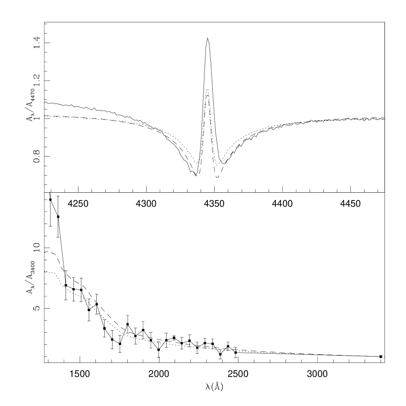
Figure 13: Comparison of models (Dotted is $\ell$=2 and dashed is ($\ell$=4, $m=0$)²) to the optical chromatic amplitudes and UV data (squares) (Kepler et al., 2000) for F5, the 71 s mode. The optical model chromatic amplitudes are created from simulated spectra and treated in the same way as the data. For both figures we used the model corresponding to T=11,750 and log(g)=8.25.

3.3 Optical Amplitudes

If the 142 s is the dominant $\ell$=4 mode, then this might explain the low amplitudes of this star’s pulsations. The measured amplitude of an $\ell$=4 mode would be limited by cancellation as the observed flux variations result from a sum across the visible surface of the star. To test this, we calculated how much brighter an $\ell$=4, $m$=0 mode would look if it appeared as an $\ell$=1, $m$=0 mode. To determine this factor we integrated both modes over the visible surface of a star seen at its pole using limb darkened models (T=11,750, log(g)=8.25) and summing the flux change over the visible wavelengths (4000-5500 Å). We concluded that an $\ell$=4 mode would be observed approximately 13 times smaller than an $\ell$=1. So, if PY Vul is dominated by an $\ell$=4 mode, its amplitude has been reduced by a factor of thirteen, meaning that our F2 would be $\sim 19.5$ mma if it were an $\ell$=1 mode. Hot DAV stars have been observed with amplitudes as high as 23 mma (see Kepler et al. (1991) and Clemens (1994)).

Assuming that the other DAVs are generally dominated by $\ell$=1 modes as deduced by Clemens (1994), we compared PY Vul to the class of DAVs after applying this scaling factor. To illustrate the results, we reproduced the plot of weighted mean period verses power from Clemens (1994) and added the location of an $\ell$=1 dominated PY Vul (Figure 14). While the actual location of PY Vul has a low amplitude, placing it below the trend of the other DAVs, a PY Vul that does not suffer the geometric cancellation of an $\ell$=4 mode would be located at the plus sign in Figure 14. Assuming PY Vul is dominated by an $\ell$=4 mode brings the amplitude of this star into line with the other stars of its class.

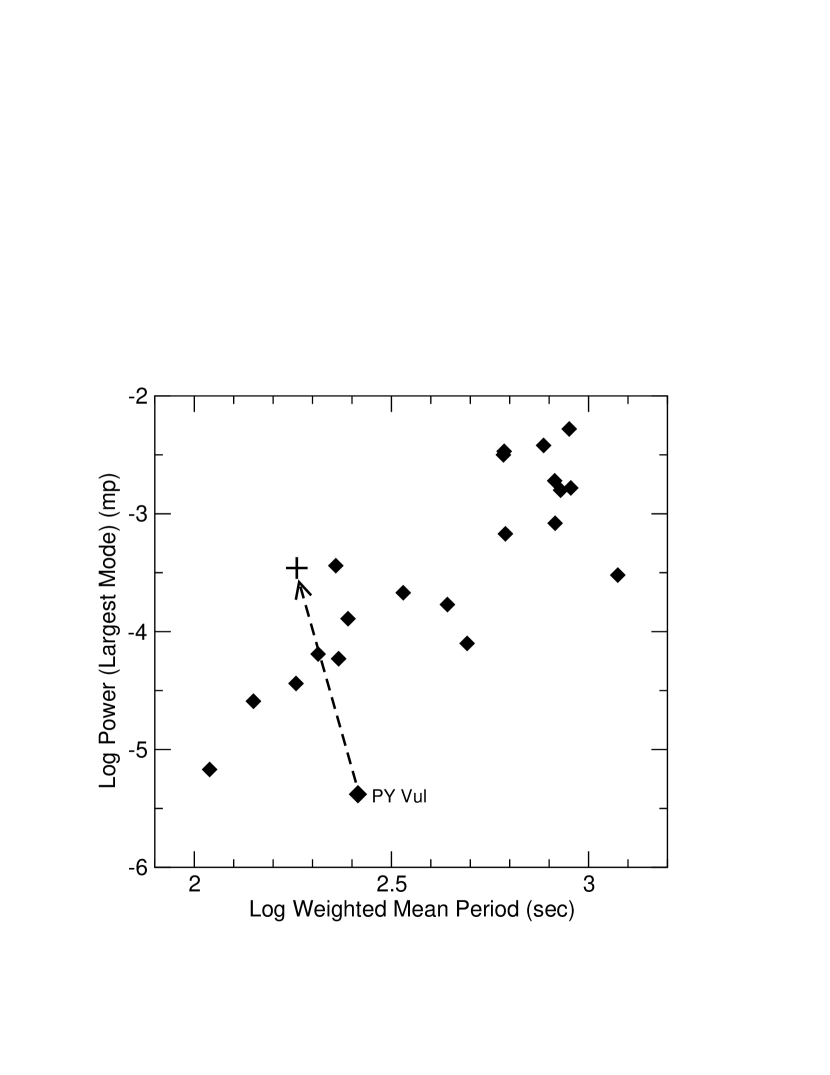
Figure 14: The power of the largest mode plotted against the weighted mean period of the DAVs. The diamonds represent the 21 DAVs studied by Clemens (1994). The observed location of PY Vul is the diamond labeled at the bottom of the plot. We propose that the reason PY Vul has a lower power than the other DAVs is that it is dominated by an $\ell$=4. The other DAVs are expected to be dominated by $\ell$=1 modes (Clemens 1994). Due to its inherent cancellation, an $\ell$=4 mode will appear 13 times smaller than an $\ell$=1 (see §3.3). We apply this scaling factor to the 142 s mode of PY Vul and adjust for the new weighted mean period (the plus sign). A PY Vul showing an $\ell$=1 mode instead of an $\ell$=4 mode agrees with the trend of the other DAVs, demonstrating that the $\ell$=4 hypothesis correctly accounts for the low amplitudes of PY Vul.

The $\ell$=4 hypothesis satisfyingly explains all the above characteristics of the pulsation spectrum of PY Vul. Our only hesitation is the failure to see 8 azimuthally split modes associated with the $\ell$=4 mode. However, we also do not see triplets for the other modes. Either the star does not excite higher $m$ modes, or is rotating so slowly that we have failed to resolve them.

4 Other Proposed Scenarios

Other suggestions have been made to explain the character of the pulsations of PY Vul. After a preliminary analysis of the same data presented here, Thompson & Clemens (2002) proposed that a large inclination could account for the low mode amplitudes. In this scenario, the 142 s mode is the first harmonic of a mostly cancelled mode found near 285 s, while the 71 s mode is the third harmonic. This hypothesis did explain the failure of the 142 s mode to rise in the UV. However, it failed to explain the behaviour of the 71 s mode in the UV. Furthermore, the 285 s parent mode required by this scenario was only marginally detected on the first night of the LRIS observations, and the extensive coverage of the WET run on PY Vul (Castanheira et al., 2004) failed to find any significant signal near 285 s. This requirement of almost total cancellation imposed by the WET data requires a very extreme inclination. To achieve the ratio between the amplitudes of the proposed 285 s and 142 s modes, the star would have to be viewed within approximately 1$\arcdeg$ of its equator. Because of this need for fine tuning and the inability to explain the UV amplitudes, this model is inferior to the $\ell$=4 hypothesis we have presented.

Castanheira et al. (2004) and Kepler et al. (2000) maintain that since the 142 s mode shows the atypical behavior in the UV, it must be due to some nonlinear effect and both the 71 s and 72 s modes are real modes. As they point out, a real mode with such short periods forces asteroseismological models to use masses near the Chandrasekhar limit in order to create an $\ell$=1, k=1 mode with such a low period (Bradley, 2001). As the mass of this star is near 0.6 M_⊙ (Castanheira et al., 2004), they conclude these modes must be $\ell$=2. They agree with Thompson & Clemens (2002) that the star must have an unfavorable inclination to create the low amplitudes and possibly the character of the 142 s mode in the UV. The largest problem with this scenario comes from the nature of the 142 s mode. Combination and harmonic modes are believed to be a result of nonlinear effects in the atmosphere of the star. However, the theories concerning the nonlinear interaction between the outer atmosphere and the pulsation modes predict the existence of harmonic modes but not sub-harmonics (Brickhill, 1992; Wu, 2001). The 142 s mode, as a subharmonic, would have to be created by some new type of mechanism that operates over every other cycle of the real, parent mode. Unlike this scenario, our $\ell$=4 hypothesis does not require the addition of any new physics. The nonlinear effects discussed by Brickhill (1992) and Wu (2001) act on the 142 s mode to create a harmonic near 71 s.

5 Conclusions

The DAV star PY Vul has a perplexing pulsation spectrum that has challenged attempts to understand the star. We have analyzed line profile variations that suggest the 142 s pulsation mode in PY Vul has a spherical degree of four. If this mode is the star’s dominant pulsation mode, then we can explain the star’s overall low pulsation amplitude by geometric cancellation without the need to invoke improbable inclinations. Furthermore, because the pulse shape harmonic of an $\ell$=4 mode has lower $\ell$ characteristics, it cancels less effectively, explaining the unusually large amplitude of the mode’s harmonic. Finally, an $\ell$=4 character of the 142 s mode and the consequent $\ell$=0,2 character of its harmonic are the very values most consistent with the UV amplitudes measured by the Hubble Space Telescope, although problems with pulsation phases remain. Together, these results yield a satisfying and unified picture of the star’s pulsations, and the only one consistent with all the data.

If our assignment of $\ell$=4 to the 142 s mode is correct, then it is a surprise since we have never before seen even $\ell$=3 and only seldom $\ell$=2. Interestingly, the assignment of $\ell$=1 to most of the modes in hot DAVs by Clemens (1994) does not apply to the 142 s region of PY Vul, which was one of two stars thought to have $\ell$$>$1. Based on period spacings alone, Clemens (1994) recognized that the 142 s or its nearby 148 s mode must be higher $\ell$ but had suspected $\ell$=2, not 4. If we are forced to consider higher $\ell$ during mode identification, then it will make that process difficult because the high $\ell$ modes are closely space in period. Fortunately, it appears that high $\ell$ modes advertise that fact by having large harmonics which may assist in their identification.

Finally, we have developed a new analysis technique for time series spectroscopy that appears to work for relatively poor signal-to-noise. The other DAVs studied by time series spectroscopy (van Kerkwijk, Clemens & Wu, 2000; Kotak, van Kerkwijk, & Clemens, 2002; Kotak et al., 2002; Kotak, van Kerkwijk, & Clemens, 2004) might benefit from re-analysis by this technqiue, which we intend to do. Also, we expect that by using this technique we will be able to extend mode identification with time-series spectroscopy to fainter stars, increasing the number of stars for which secure mode identification is possible.

References

- Bradley (2001) Bradley, P. A. 2001, ApJ, 552, 326
- Brickhill (1991) Brickhill, A. J. 1991, MNRAS, 251, 673
- Brickhill (1992) Brickhill, A. J. 1992, 259, 519
- Castanheira et al. (2004) Castanheira, B. G., et al. 2004, A&A, 413, 623
- Clemens (1994) Clemens, J. C. 1994 PhD Thesis
- Clemens, van Kerkwijk, & Wu (2000) Clemens, J. C., van Kerkwijk, M. H., Wu, Y. 2000, MNRAS, 314, 220
- Horne & Baliunas (1986) Horne, J. H., & Baliunas, S. L. 1986, ApJ, 392, 757
- Kepler et al. (1991) Kepler, S. O. et al. 1991, ApJL, 378, L45
- Kepler et al. (2000) Kepler, S. O., Robinson, E. L., Koester, D., Clemens, J. C., Nather, R. E., &Jiang, X. J. 2000, ApJ, 539, 379
- Kotak, van Kerkwijk, & Clemens (2002) Kotak, R., van Kerkwijk, M., & Clemens, J. C. 2002, A&A, 388, 219
- Kotak et al. (2002) Kotak, R., van Kerkwijk, M. H., Clemens, J. C., & Bida, T. A. 2002 A&A, 391, 1005
- Kotak, van Kerkwijk, & Clemens (2004) Kotak, R., van Kerkwijk, M. H., & Clemens, J. C. 2004, A&A, 413, 301
- Ising & Koester (2001) Ising, J. & Koester, D. 2001, A&A, 374, 116
- McGraw et al. (1981) McGraw, J. T., Fontaine, G., Dearborn, D. S. P., Gustafson, J., Lacombe, P. & Starrfield, S. G. 1981, 250, 349
- Oke et al. (1995) Oke, J. B. et al. 1995, PASP, 107, 375
- Robinson, Kepler, & Nather (1982) Robinson, E. L., Kepler, S. O., & Nather, R. E. 1982, ApJ, 259, 219
- Robinson et al. (1995) Robinson, E. L. 1995, ApJ, 438, 908
- Thompson & Clemens (2002) Thompson, S. E. & Clemens, J. C. 2003, Asteroseismology Across the HR diagram (Kluwer Academic Publishers), Astrophy. Space Sci. 284, P573
- Thompson et al. (2003) Thompson, S. E., Clemens, J. C., van Kerkwijk, M. H., & Koester, D. 2003, ApJ, 289, 921
- Tody (1986) Tody, D. 1986, Proc. SPIE, 2198, 362
- van Kerkwijk, Clemens & Wu (2000) van Kerkwijk, M. H., Clemens, J. C., & Wu, Y. 2000, MNRAS, 314, 209
- Winget (1982) Winget, D. E. 1982, Ph.D. Thesis
- Winget & Fontaine (1982) Winget, D. E., & Fontaine, G. 1982, in Pulsations in Classical and Cataclysmic Variables, Ed. J. P. Cox & C. J. Hansen (Boulder: JILA), 46
- Wu (2001) Wu, Y. 2001, MNRAS, 323, 248
- Wu & Goldreich (1999) Wu, Y. & Goldreich, P. 1999, ApJ, 519, 783