Assessing the effects of foregrounds and sky removal in WMAP

Abstract

Many recent analyses have indicated that large scale WMAP data display anomalies that appear inconsistent with the standard cosmological paradigm. However, the effects of foreground contamination, which require elimination of some fraction of the data, have not been fully investigated due to the complexity in the analysis. Here we develop a general formalism of how to incorporate these effects in any analysis of this type. Our approach is to compute the full multi-dimensional probability distribution function of all possible sky realizations that are consistent with the data and with the allowed level of contamination. Any statistic can be integrated over this probability distribution to assess its significance. As an example we apply this method to compute the joint probability distribution function for the possible realizations of quadrupole and octopole using the WMAP data. This 12 dimensional distribution function is explored using the Markov Chain Monte Carlo technique. The resulting chains are used to asses the statistical significance of the low quadrupole using frequentist methods, which we find to be 3-4%. Octopole is normal and the probability of it being anomalously low or as low as WMAP reported value is very small. We address the quadrupole-octopole alignment using several methods that have been recently used to argue for anomalies, such as angular momentum dispersion, multipole vectors and a new method based on feature matching. While we confirm that the full sky map ILC suggest an alignment, we find that removing the most contaminated part of the data also removes any evidence of alignment: the probability distributions strongly disfavor the alignment. This suggests that most of the evidence for it comes from non-Gaussian features in the part of the data most contaminated by the foregrounds. We also present an example, that of octopole alignment with the ecliptic, where the statistical significance can be enhanced by removing the contamination.

I Introduction

The large scale structure of the WMAP data (Efstathiou, 2003) has received a lot of attention since the first data release. Some authors have focused on the seemingly low values of quadrupole and octopole Efstathiou (2003, 2004); Tegmark et al. (2003); Slosar et al. (2004), and their alignment (de Oliveira-Costa et al., 2004; Schwarz et al., 2004), while others considered various asymmetries in the data (Eriksen et al., 2003, 2004; Hansen et al., 2004a, b). Some of these analyses are performed on one of the available full sky WMAP maps, either the original WMAP Internal Linear Combination Map (ILC) or an alternative map Tegmark et al. (2003), which we will refer to as TOH map. The full sky maps have the advantage that the harmonic analysis is unique, which facilitates investigation and assessment of statistical significance. We note that Eriksen et al. (2004) prudently warn against the usage of the foreground corrected full-sky maps and use appropriate Monte-Carlo simulations.

However, full sky maps are not free of contamination, as was clearly emphasized by the WMAP team warning that their ILC map should not be used for science purposes. These are dominated by galactic foregrounds such as dust, synchrotron or free-free emission. For this reason the power spectrum analysis is done on cut sky, where about 15-25% of most contaminated data in the galactic plane is removed. Even outside this region there are residual uncertainties associated with imperfections of the foreground removal. If ignored they may cause spurious alignments or other anomalies that appear statistically significant under the assumption that CMB is a Gaussian random field.

In this paper we revisit the statistical significance of these tests using a different approach. Rather than ignoring the effects of foregrounds we try to take them into account explicitly by exploring the uncertainties they induce in the measurements of the multipole moments $a_{\ell m}$. We assess this uncertainty by determining the joint multi-dimensional probability distribution function for the true sky multipole moments. Once these are determined we can apply them to the statistics of choice to obtain their values in the presence of uncertainties associated with imperfect foreground removal or sky cuts. We do not address the question of the meaning of a given statistic: all of the statistics are a-posteriori and their statistical significance is difficult to assess. Instead, our goal is to compare the values of these statistics with and without the inclusion of foreground uncertainties to see if including the latter changes the conclusions significantly.

In this paper we are interested in large scale features, so we focus exclusively on quadrupole and octopole. This allows us to perform several tests. First, we can revisit the question of whether the quadrupole and octopole are low in the presence of additional uncertainties associated with the foregrounds and sky cuts. Secondly, we can test how robust results of methods for measuring the alignment of quadrupole and octopole are, once these uncertainties are taken into account. We do this by applying several of existing statistics, as well as a new one we developed. Finally, we also explore the alignment of the large scale features with specific directions in the sky, such as that of ecliptic plane.

II Method

We need to distinguish between two types of uncertainties. The theory of CMB fluctuations can only predict ensemble averages of the power spectrum of CMB fluctuations. Given the statistical description of initial fluctuations in the form of a power spectrum and parameters of a given cosmological model it is only possible to predict the power spectrum of the CMB fluctuations averaged over all possible realizations of the universe. Since there is only one CMB sky that we can directly measure, there is a corresponding uncertainty in our inference of the true cosmic power spectrum. This uncertainty is often referred to as cosmic variance.

In terms of multipole moments $a_{\ell m}$, for an idealized experiment with full sky coverage and no foreground contamination or noise, their values can be determined precisely. In this case the only uncertainty is the cosmic variance. However, if there is noise or contamination we may not be able to measure precisely the individual multipole moments either. This introduces an additional level of uncertainty. For the power spectrum analysis such an uncertainty is automatically accounted for in the likelihood analysis, where sky-cuts and foreground uncertainties can be included in the likelihood calculations without determining the actual values of multipole moments. For other more complicated statistics one must determine the probability distribution of the multipole moments first and then apply these to the statistic of interest.

II.1 Probability distribution of the multipole moments

In general determining the full probability distribution of multipole moments can be numerically challenging, as the multipole moments will be correlated and their number will grow as the square of the number of considered multipoles. Here we focus on large scales only, where quadrupole and octopole dominate. Their joint probability distribution function has $12$ degrees of freedom. We use Markov Chain Monte Carlo in the form of the simplest Metropolis algorithm (Metropolis et al., 1953) with a fixed Gaussian width proposal function. Since the likelihood evaluations are very fast this simple method is sufficient. We note that the posterior distribution $p(a_{\ell m})$ is gaussian by construction and can be fully constrained with just a few likelihood evaluations. This can considerably speed up the calculations, but is not really needed for our analysis where we focus on the lowest multipoles only.

In order to make valid constraints on various realizations of the quadrupole and octopole we need to devise a way of calculating the likelihood of a given $a_{2m}$s and $a_{3m}$s in the presence of the instrumental noise, fluctuations due to the power in the higher multipoles and foreground contamination. In analogy with the common $\chi^{2}$ analysis, the likelihood of a given model is the probability that the residuals between the theoretical map for a given theoretical model (i.e. a map corresponding to a quadrupole and octopole) and the measured map are a possible noise realization. Therefore, the likelihood can be written as:

$$\log L=-\frac{1}{2}\mathbf{(d-d_{T})^{T}(C^{\rm total})^{-1}(d-d_{T})}+D$$ (1)

where $\mathbf{d_{T}}$ is the theoretical map data-vector

$$(\mathbf{d_{T}})_{i}=\sum_{\ell=2,3}\sum_{m=-\ell\ldots\ell}Y_{\ell m}(\mathbf{n}_{i})a_{lm},$$ (2)

with $\mathbf{n}_{i}$ being the unit vector in the direction of the $i$-th data-point and $D$ is an unimportant constant.

The covariance matrix $\mathbf{C^{\rm total}}$ is the total covariance matrix, which can be broken into several parts as follows:

$$\mathbf{C}^{\rm total}=\mathbf{C}+\mathbf{N}+\lambda(\mathbf{C}^{\rm dust}+\mathbf{C}^{\rm synch}+\mathbf{C}^{\rm free-free} +$$

$$\mathbf{C}^{\ell=0}+\mathbf{C}^{\ell=1})$$ , (3)

The main contribution is the noise due to fluctuations in the multipoles higher than recovered ones:

$$C_{i,j}=\sum_{\ell=4}^{\infty}\frac{2\ell+1}{4\pi}C_{\ell}P_{\ell}(\cos\theta_{i,j})B_{\ell},$$ (4)

where the sum starts at the lowest multipole which is not being recovered, $P_{\ell}$ is the Legendre Polynomial of order $\ell$, $B_{\ell}$ is the beam smoothing and $\theta_{i,j}$ is the angle between $i$th and $j$th point on the sky. We denote with $\mathbf{N}$ the instrumental noise matrix, which for $l=2,3$ is small compared to other sources of noise.

The matrices $\mathbf{C}^{\rm dust}$, $\mathbf{C}^{\rm synch}$ and $\mathbf{C}^{\rm free-free}$ are foreground contamination matrices, given by

$$\mathbf{C}^{\rm foreground}=\mathbf{LL}^{\dagger},$$ (5)

where $\mathbf{L}$ is the foreground template vector. As discussed in previous paper Slosar et al. (2004), the linear modes that correlate with the foreground template vector are effectively marginalized out in the limit of $\lambda\rightarrow\infty$. This is not the only option if one has additional information on the probable amplitude of these foregrounds, so in this paper we also try $\lambda=1$, corresponding to the case where multi-frequency information in WMAP does provide some information on their amplitude, but with an error of order unity compared to the best fit value. Finally, we also marginalize the residual dipole and monopole in the map with $\lambda\rightarrow\infty$, since we have no external information on their value.

This method allows us to calculate the likelihood of a given realization of a quadrupole and octopole in the presence of power in higher multipoles, foregrounds and monopole/dipole contamination. We explore the likelihood surface by making steps in a random direction, at each step deciding on whether to accept the new event based on the likelihood ratio relative to previous event. This MCMC sampling of the likelihood surface results in a 12 dimensional probability distribution of multipole moments, which is consistent with the data and with the allowed level of foreground contamination. Each MCMC element consists of a realization of multipole moments defined on the uncontaminated and uncut sky, so one can apply any statistic of choice to a given realization without having to worry about contamination, noise or sky cuts and various effects associated with implied priors. By averaging over MCMC elements one is performing marginalization over the full probability distribution. A related method has been proposed in Wandelt et al. (2003) and Wandelt (2004).

It is important to realize that the inverse of the covariance matrix is calculated just once and therefore the likelihood evaluation is a very fast process. In fact, the entire MCMC process takes a few hours on a modern PC workstation. The method is trivially extended to higher multipoles. If a map has $N$ pixels, it is completely defined by the $\ell_{\rm max}\propto N^{1/2}$ multipoles. Assuming the time required to calculate a candidate map scales as $N$ (if we are moving in a specific $a_{\ell,m}$ direction) and that the MCMC chain is limited by the random walk rather than shot noise in the sample density, then a very favorable scaling of $N^{3/2}$ is obtained for reconstructing all multipoles in the map. However, it is very likely that the method will be limited by the very complicated multi-modal likelihood shape in the case of higher multipole reconstruction.

II.2 Choice of maps and foreground templates

We focus on three increasingly conservative combinations to asses the stability of statistical inferences. All maps are smoothed using $5^{\circ}$ FWHM beam and down-sampled to the nside=16 Healpix map. Our three datasets in order of increasing conservativeness are:

• ILC dataset contains the full-sky ILC map. Noise is ignored and so are foreground contaminations. This dataset can be used to compare our results with the previously reported results and to asses whether the methods produces the expected results, but is likely to be too contaminated for results to be reliable.

• Wd dataset takes the W channel data, applies the Kp2 mask, subtracts the MEM derived Free-Free foreground and marginalizes over MEM derived Dust template (using $\lambda=1$ and $\lambda=\infty$).

• Vdfs takes the V channel map, applies the Kp2 mask, and marginalizes over all three foreground templates of Dust, Free-Free and Synchrotron emission.

We have run the MCMC process until at least 500000 independent samples were obtained and discarded first 10000 samples. The process is very fast and a large number of samples ensures that the chain is well converged. We checked this by comparing results of the first quarter of samples with that of the last quarter.

II.3 Priors and implied priors

Multipole moments $a_{\ell m}$ are drawn from a Gaussian distribution with variance $C_{\ell}$. The values of $a_{\ell m}$ are in general complex, but the requirement that the observed sky is a real quantity demands that $a_{\ell m}=a_{\ell-m}^{\ast}$. This requires that the imaginary part of $a_{\ell 0}$ vanishes and thus we are left with $2\ell+1$ degrees of freedom. We introduce the symbol $D_{\ell}$ to describe the “measured power spectrum” on a given sky,

$$D_{\ell}={1\over 2l+1}\sum_{m}|a_{\ell m}|^{2}.$$ (6)

Our MCMC process takes flat priors on the values of each of the imaginary and real components of $a_{\ell m}$, which are wide enough so that they do not affect the posterior probability distribution $p(a_{\ell m})$. This, however, implies a non-flat prior on the derived probability distribution for $D_{\ell}$.

This can be calculated as follows. In the $2\ell+1$ dimensional space spanned by $(a_{\ell,0}$, $\sqrt{2}{\rm\ Re\ }(a_{\ell,1})$, $\sqrt{2}{\rm\ Im\ }(a_{\ell,1})$, …$)$ the points of constant $D_{\ell}$ lie on the hyper-sphere with radius $R=((2\ell+1)D)^{1/2}$. The number of states corresponding to the volume of the shell of thickness ${\rm d}R$ determines the number of available states and therefore the implied prior is given by

$$p_{\rm implied}(D_{\ell}){\rm d}D_{\ell}\propto R^{2\ell}{\rm d}R\propto D^{\ell-\frac{1}{2}}{\rm d}D.$$ (7)

In particular, the implied prior for the quadrupole is $p_{\rm implied}(D_{2})\propto D^{3/2}$ and for the octopole $p_{\rm implied}(D_{3})\propto D^{5/2}$.

As usual in such analyses, if the data were perfect the assumed prior would be irrelevant, while in the opposite limit all information comes from priors. It seems however unlikely that the assumed priors would affect our results on alignments (discussed below), as long as the priors do not introduce any correlations between the multipole moments. Therefore, we take these implied priors into account when calculating the estimates of the statistical significance of quadrupole and octopole (because a flat $C_{\ell}$ prior is usually assumed in analyses of this kind), but not when assessing the alignment of quadrupole and octopole.

In the rest of this paper we will also use symbols $\mathsf{C}_{\ell}$ and $\mathsf{D}_{\ell}$ which correspond to a more conventional normalization of $C_{\ell}$ and $D_{\ell}$

$$\mathsf{C}_{\ell}=\frac{C_{\ell}\ell(\ell+1)}{2\pi}$$ (8)

$$\mathsf{D}_{\ell}=\frac{D_{\ell}\ell(\ell+1)}{2\pi}.$$ (9)

II.4 Consistency check: measured versus true power spectrum

The $D_{\ell}$ (equation 6) is $\chi^{2}$ distributed with $2\ell+1$ degrees of freedom,

$$p(D_{\ell}|C_{\ell})=\left[C_{\ell}\Gamma\left(\ell+\frac{1}{2}\right)\right]^{-1}\exp\left(\frac{D_{\ell}}{C_{\ell}}\right)\left[\frac{D_{\ell}}{C_{\ell}}\right]^{\ell-\frac{1}{2}}.$$ (10)

However, we measure $D_{\ell}$ and assuming a flat prior on $C_{\ell}$ the Bayes theorem says:

$$p(C_{\ell}|D_{\ell})\propto p(D_{\ell}|C_{\ell})$$ (11)

For an idealized experiment with full sky coverage and no foreground contamination or noise, the value of $D_{\ell}$ can be determined precisely and therefore one is only constrained by the cosmic variance from Equations (10) and (11) as discussed in the introduction. For a real experiment, one must marginalize over this uncertainty

$$p(C_{\ell})=\int p(C_{\ell}|D_{\ell})p(D_{\ell}){\rm d}p(D_{\ell})$$ (12)

Given the probability distribution function for $a_{\ell m}$ allows one to calculate the probability distribution function for $p(D_{\ell})$ using

$$p(D_{\ell})=\int\cdots\int\frac{\sum_{m}|a_{\ell m}|^{2}}{2\ell+1}P\left(a_{00},\ldots a_{\ell_{\rm max}\ell_{\rm max}}\right)$$

$$\times{\rm d}a_{\ell 0}\ldots{\rm d}a_{\ell\ell},$$ (13)

where $\ell_{\rm max}$ is the maximum $\ell$ for which this distribution is recovered. Combining the expressions above gives us $p(C_{\ell})$.

As mentioned in the introduction the various power spectrum determination procedures such as PCL (see e.g. (Hivon et al., 2002)) and QML (see e.g. (Tegmark, 1997)) estimators or the exact methods using matrix inversion already take into account the cosmic variance to derive $p(C_{\ell})$. As a consistency check we compare the $p(\mathsf{C}_{2})$ derived from our chains to that of the exact likelihood analysis performed in Slosar et al. (2004). We do this in the following manner. We calculate the $p(\mathsf{D}_{2})$ using our MCMC chains. The inferred probability distribution is then multiplied by $D^{-3/2}$ to take into account the effect of the implied prior effect as described in the section II.3. Finally we numerically integrate Equation (12) to get the probability distribution $p(\mathsf{C}_{2})$. The resulting $p(\mathsf{C}_{2})$ for the Vdfs case is shown in Figure 1, together with the $p(\mathsf{C}_{2})$ obtained by calculating the exact likelihood using the matrix formalism. The two curves are in a good agreement. This confirms that the method works as expected.

Figure 1: This Figure shows the probability distribution function for the true quadrupole in Vdfs case, calculated using two methods. The solid line correspond the $p(\mathsf{C}_{2})$ distribution function derived using MCMC chains, while the dashed line corresponds to the distribution derived using the exact likelihood calculation by matrix inversion. The two curves are in a good agreement indicating that the method is numerically robust.

II.5 Fitting individual foregrounds

We have also tested the behavior of the system if one takes the amplitudes of the foregrounds to be additional variables of the system. In this case, the marginalization is performed by explicit fit to the amplitudes of these foregrounds. We have taken the V frequency data, applied the KP2 cut and used the standard foreground templates used by the WMAP team: the 408MHz Haslam synchrotron radiation map (Haslam et al., 1982),H-$\alpha$ map from Finkbeiner (2003) as a tracer of free-free emission and the FDS dust template based on Finkbeiner et al. (1999). We used these templates instead of MEM derived maps to make the inferred amplitudes as statistically independent as possible and thus avoid complications associated with signal-noise correlations which become apparent when using MEM foreground maps. Additionally we imposed constraints that all amplitudes must be positive. The resulting 12+3 dimensional probability space is explored using the standard MCMC procedure. We show the resultant amplitudes in Figure 2. In this plot, the amplitudes have been rescaled to average to one as the absolute numbers are not important for our application (templates give only the flux ratio between the pixels). The data determine the amplitude of the dust and free-free emissions fairly accurately, but the amplitude of the synchrotron is only poorly constrained and consistent with 0. This is what is expected, since the synchrotron is not anticipated to be a major contaminant at the frequencies of the V channel.

Figure 2: This figure shows the inferred amplitudes of foreground maps when used to fit the data. The x axis has been rescaled to average to one. See text for further discussion.

We have also investigated degeneracy directions which might exist between various templated amplitudes and the values of $\mathsf{D}_{2}$ and $\mathsf{D}_{3}$. Template amplitudes are nearly completely uncorrelated between each other and with the multipole amplitudes. The only marginally significant correlation exists between the Dust amplitude and the value of $\mathsf{D}_{2}$. This is shown in Figure 3.

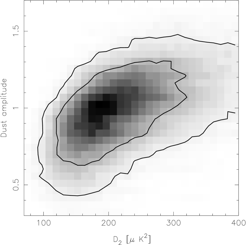
Figure 3: This Figure shows the two-dimensional distribution of the probability on the $\mathsf{D}_{2}$ - Dust amplitude plane. Contours correspond to 1 and 2-sigma confidence limits. See text for further discussion.

III Results

III.1 Distributions for $\mathsf{D}_{2}$ and $\mathsf{D}_{3}$

In Figure 4 we show the marginalized one-dimensional distributions for $\mathsf{D}_{2}$ and $\mathsf{D}_{3}$ for the three cases and the Wd case with $\lambda=1$. These show several interesting features. The ILC map gives values of $\sim 195\mu K^{2}$ for the quadrupole and $\sim 1050\mu K^{2}$ for the octopole, in a good agreement with results obtained previously on the same map using the QML estimator Efstathiou (2004). Zooming up into the region actually reveals the probability distribution is a narrow Gaussian with FWHM of a few $\mu K^{2}$, consistent with the effect of finite pixelization, etc. The confidence limits on the two parameters widen with the inclusion of sky cuts and the increasing amount of foreground correlated modes being marginalised out. We note that Wd case is very similar for $\lambda=1$ and $\lambda\rightarrow\infty$. This is consistent with our findings in Section II.5. The former sets the uncertainty in the foreground amplitude to the $O(1)$, while the latter effectively marginalises over the foreground amplitude probability given the data, which we have shown to be of the order $O(1)$. Therefore, we will limit our discussion to $\lambda\rightarrow\infty$ in the rest of this paper. It is interesting to note that while including more uncertainty in foreground subtraction (Vdfs versus Wd) makes the distribution broader, it also pushes the median to lower values.

Figure 4: This Figure shows the distribution for $\mathsf{D}_{2}$ and $\mathsf{D}_{3}$ for the following four cases: ILC (vertical lines), Wd (thin line), Wd with $\lambda=1$ (thick dashed line) and Vdfs (thick line).

We also plot the 2-dimensional distribution on the $\mathsf{D}_{2}$-$\mathsf{D}_{3}$ plane for the most conservative Vdfs case in Figure 5. $\mathsf{D}_{2}$ and $\mathsf{D}_{3}$ are nearly completely uncorrelated, in accordance with previous findings.

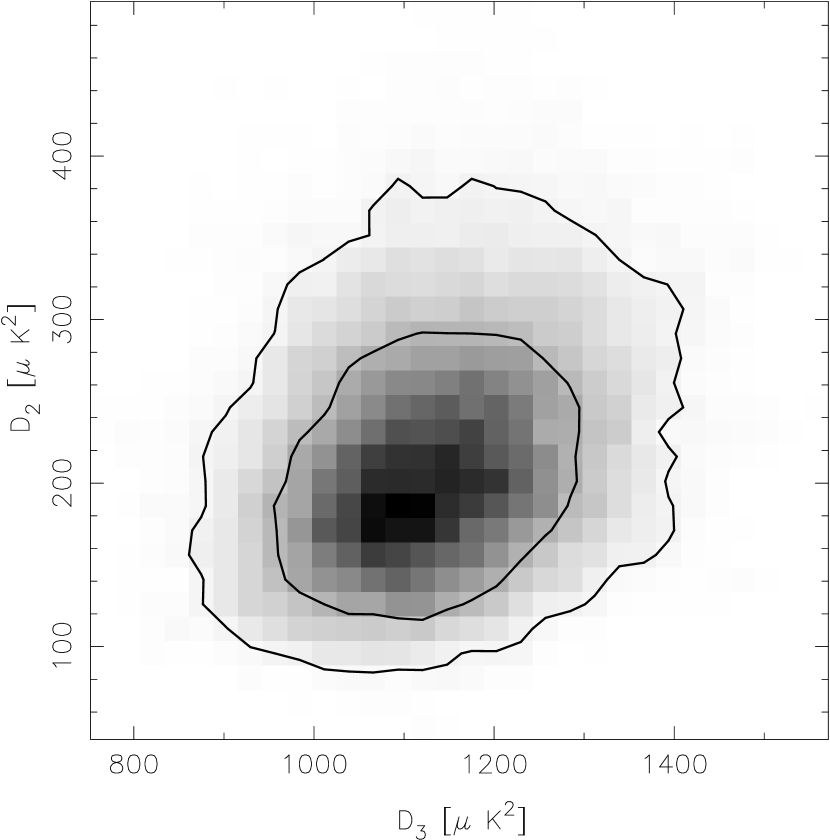
Figure 5: This Figure shows the two-dimensional distribution of the probability on the $\mathsf{D}_{2}$-$\mathsf{D}_{3}$ plane for the Vdfs case. Contours correspond to one-sigma and two sigma confidence limits.

III.2 How low are the quadrupole and octopole?

Reference Efstathiou (2003) proposes two methods for assessing the statistical significance for the low quadrupole, assuming that the $\mathsf{D}_{2}$ distribution is known. The Bayesian estimate is concerned with the probability that $\mathsf{C}_{2}$ is greater that its concordant value ($1150\mu K^{2}$) given the value of $\mathsf{D}_{2}$. This is just the integral of the $p(\mathsf{C}_{2})$ from its concordant value upwards and therefore our MCMC chains do not add new information, as the $p(\mathsf{C}_{2})$ can already be obtained from the exact likelihood evaluation shown in Figure 5 of the reference Slosar et al. (2004). Here we highlight the fact that the likelihood at high values of true quadrupole is very slowly decreasing and as a result the probability depends on the adopted prior. We quote these results in the Table 1.

Table 1: This table shows the Bayesian estimates for the probability of the low quadrupole assuming a narrow (uniform between 0 and 2000 $\mu K^{2}$) and a wide (uniform between 0 and 10000 $\mu K^{2}$) prior on the value of $\mathsf{D}_{2}$.

Dataset	Narrow prior	Wide prior
$p(\mathsf{D}_{2})=\delta(\mathsf{D}_{2}-123\mu K^{2})$	5.0%	8.5%
ILC	9.1%	16%
Wd	11%	18%
Vdfs	8.8%	15%

Frequentist estimate is concerned with the probability that the value of $\mathsf{D}_{2}$ is as small or smaller than the observed $\mathsf{D}_{2}$ given that the value of $\mathsf{C}_{2}$ takes its concordant value ($1150\mu K^{2}$). We calculate a “frequentist” estimate integrating over the probability distribution for $p(\mathsf{D}_{2})$. We emphasize that this is not a real frequentist estimate, since a true frequentist statistic is never a-posteriori. We have also corrected for the Bayesian implied prior on the values of $\mathsf{D}_{2}$ as discussed in the Section II.3.

The results are shown in Table 2. We note that the values are a factor of a few higher than the original WMAP estimate and do not depend much on which method we use. The ILC value of $\mathsf{D}_{2}\sim 195\mu K^{2}$ is somewhat higher, but consistent with the original WMAP value of $154\pm 70\mu K^{2}$ Bennett et al. (2003). We note, however, that the number quoted in the official power spectrum file is considerably lower, $123\mu K^{2}$. The probability for the frequentist estimate rises from 1% to about 3% with the larger value, which is already a major increase. Taking into account the non-negligible width in the probability distribution function for $\mathsf{D}_{2}$ for the Wd and Vdfs does not change the probability significantly. Note that the WMAP value of $123\mu K^{2}$ is perfectly acceptable for the more conservative Vdfs analysis, which marginalizes over 3 foreground templates, but appears nearly excluded from Wd analysis. In other words, if one assumes W map with KP2 mask and assumes the foreground uncertainties are associated only with the dust template then the probability for the actual quadrupole on the sky $\mathsf{D}_{2}$ to be below $123\mu K^{2}$ is extremely small, less than 0.01%.

Octopole results show a similar pattern, except that octopole is not low compared to standard model. The ILC value of $\sim 1050\mu K^{2}$ is in near perfect agreement with the concordance model value of around 1100$\mu K^{2}$. This is changed into a broader distribution by the more conservative treatments, with the peak values close to the ILC value around 1100$\mu K^{2}$ and the width of about 150$\mu K^{2}$ FWHM. Both distributions are similar, so the details of foreground marginalization do not appear very important here. However, the low octopole value reported by WMAP, $611\mu K^{2}$, is not within the allowed range even for the most conservative treatment and there is not a single MCMC sample that would give a value this low. It is not clear what the cause for this discrepancy with WMAP values is, but one possible culprit is the estimator used by WMAP, which is noisier than the optimal maximum likelihood estimator and which thus can lead to an estimate that differs significantly from the actual value Efstathiou (2004). In conclusion, quadrupole is somewhat but not anomalously low, its probability is around 3-4%, while octopole is perfectly normal and there is essentially zero probability for it to be as low as WMAP reported value.

Table 2: This table shows the “frequentist” estimates of the probability of low quadrupole. See text for further discussion.

Dataset	Frequentist probability
$p(\mathsf{D}_{2})=\delta(\mathsf{D}_{2}-123\mu K^{2})$	1.1%
ILC:     $p(\mathsf{D}_{2})=\delta(\mathsf{D}_{2}-195\mu K^{2})$	3.0%
Wd	4.0%
Vdfs	3.1%

IV The quadrupole and octopole alignment

In this section we will evaluate the statistical significance of various statistical measures which have been used to claim the alignment between quadrupole and octopole.

Once again, we would like to stress the a-posteriori nature of the estimators discussed below. In an idealized scientific experiment, estimators and methods to be used to distinguish between various theoretical models are known before the results and thus the inferred constraints are objective in the sense that methods are “blind” with respect to the data. In practice, however, progress is often made by spotting patterns in the data which are not predicted by the theory. One must be careful, however, when interpreting results which are concerned with attempts to quantify the statistical significance of the spotted regularities. The estimators and methods used in the latter case are by construction biased towards showing a positive detection. In the remaining part of this paper we simply wish to address the sensitivity of various estimators to the uncertainties caused by foreground subtraction and sky cuts. We do not try to asses the question of meaning of probabilities associated with various methods.

IV.1 Angular momentum dispersion

Authors of de Oliveira-Costa et al. (2004) have defined a unique axis for each multipole motivated by quantum-mechanical considerations. For each $\ell$ the axis $\mathbf{v}$ is defined as one that maximizes the angular momentum dispersion (AMD) given by

$$K=\sum_{m}m^{2}|a_{\ell m}|^{2}.$$ (14)

By examining the absolute value of the dot-product between the AMD vectors for quadrupole and octopole

$$d=|\mathbf{v_{\ell=2}\cdot v_{\ell=3}}|,$$ (15)

one can asses the statistical significance for their alignment. The absolute value takes into account the fact that these vectors are head-less (i.e. their negative also maximize $K$). It can be easily shown that the distribution for $d$ is uniform between zero and one if AMD vectors are randomly distributed on the sky.

We have implemented the code that finds the AMD vectors for quadrupole and octopole using the matrix transformations that can be found in the appendix D of de Oliveira-Costa et al. (2004). We determine the maximum value of $K$ by numerical maximization rather than calculating the values of $K$ on a Healpix grid. Using values for $a_{2m}$ and $a_{3m}$ from de Oliveira-Costa et al. (2004) we are able to reproduce their value of $d=0.986$.

When this method is applied to our MCMC chains we obtain probability distribution function for $d$. This probability distribution function can, in principle, be used to compare the Bayesian evidence for aligned quadrupole and octopole model ($d=1$) with a standard model ($d$ being uniform between 0 and $1$). We plot our results in Figure 6. These results are worthy some discussion. First, in the case of ILC map we get the value of $d=0.95$ which is consistent with de Oliveira-Costa et al. (2004) and the small difference between $\sim 0.95$ and $\sim 0.986$ is caused by the difference between the WMAP ILC map and the full-sky TOH map. For the Wd case, we see that the moderately high values of $d$ are still preferred, but the distribution develops a large tail towards smaller values of $d$. It is interesting, however, that the very high values of $d$ are strongly disfavored. Values as high as $0.98$ are allowed, but the values of $d\sim 1$ seem to be strongly rejected. In the Vdfs case all evidence for high values of $d$ seem to vanish. The probability for $d>0.98$ is 0.11% for Wd and 0.5% for Vdfs, compared to 2% probability for the random distribution. The corresponding numbers for $d>0.95$ are 2.3% and 1.6%, compared to 5% probability if random. The probability for alignment exceeding these two values in the data is below what it would be in the complete absence of the data (random case). Thus the data do not show any evidence for alignment once the foreground uncertainties are included in the analysis.

A more detailed inspection reveals that the quadrupole vectors remained fairly well defined, while the vectors for octopole developed a strong plane degeneracy. This degeneracy is responsible for the decrease in the statistical evidence for alignment. The main conclusion from this investigation is that the alignment is not robust against different treatments of foreground subtraction and that a complete alignment is strongly disfavored by the data.

Figure 6: The probability distribution function for the alignment of quadrupole and octopole using the maximum angular momentum dispersion method. The value of $1$ indicates fully aligned vectors, while a random model would correspond to uniform probability distribution. See text for further discussion.

IV.2 Multipole Vectors

Another method to explore the alignments are the multipole vectors Copi et al. (2003). It is based on the idea that every multipole of the order $\ell$ is fully determined by $\ell$ headless vectors $\mathbf{\hat{v}}^{\ell,i}$ such that

$$\sum_{m}Y_{\ell m}\left(\hat{e}\right)a_{\ell m}=A^{(\ell)}\prod_{i=1}^{\ell}\left(\mathbf{\hat{v}}^{\ell,i}\cdot\mathbf{\hat{e}}\right).$$ (16)

Pairs of these vectors can be used to form oriented areas, by taking a cross-product between them:

$$\mathbf{w}^{\ell,i,j}=\mathbf{\hat{v}}^{\ell,i}\times\mathbf{\hat{v}}^{\ell,j}.$$ (17)

We thus have one such “area” vector for the quadrupole and three for the octopole. If one takes the dot-products between $\mathbf{w}^{2,1,2}$ (quadrupole) and $\mathbf{w}^{3,i,j}$ (three octopole vectors) and orders them in decreasing magnitude one obtains three numbers denoted $A_{1}$, $A_{2}$ and $A_{3}$. A recent paper (Schwarz et al., 2004) claims that these values are anomalously high, indicating the alignment between quadrupole and octopole. Since the multipole vectors are well defined only on full sky the analysis has been applied to full sky ILC maps, which may have residual contamination due to imperfect foreground subtraction. Our method is ideal to address these concerns in a systematic fashion.

We have calculated the multipole vectors for our chains using the publicly available code (Schwarz et al., 2004). We used these vectors to obtain the probability distributions for $A_{i}$ in all cases of our chains, as well as on a Monte-Carlo simulation of 150000 random realizations of the sky to get the null-hypothesis distribution for $A_{i}$. The results are plotted in Figure 7. Applying the method to the full sky TOH map we are able to reproduce the results in Schwarz et al. (2004). Note that the results are more significant for the dynamic quadrupole corrected than dynamic quadrupole uncorrected map (see Tegmark et al. (2003) for detailed description of the differences between these). All of the $A_{i}$ values, and $A_{3}$ in particular, are high. Applying this analysis to ILC map we find similar, although somewhat less statistically anomalous, results.

We investigate next the effect of foreground uncertainty on these statistics. It is clear from figure 7 that introducing these uncertainties significantly degrades the statistical significance. This is particularly clear for $A_{3}$, which has a value in excess of 0.7 for TOH, while neither Wd not Vdfs probability distributions extend this high. The probability for $A_{3}>0.7$ is 0.09% for Wd and 0.02% for Vdfs, compared to 0.2% for the random case. Once again, adding the observations reduces the probability of an alignment (defined here as $A_{3}>0.7$) relative to no observations. This is not very sensitive to the value we choose for alignment, i.e. we find similar effect for $A_{3}>0.6$ and $A_{3}>0.5$. Other parameters give similar results, as is clear from Figure 7. We thus see no evidence that these parameters are anomalously high in the data compared to the random case, once the foreground uncertainties are accounted for. Thus, any evidence for the anomalously high value in the full sky map must come from the region that is strongly affected by the sky cuts or foreground subtraction. In other words, the evidence for the anomaly comes from the region that is most likely to be contaminated by foregrounds and so is not a robust feature in the data.

Figure 7: The probability distribution for $A_{i}$ measures of alignment using multipole vectors. The top line shows the prior distribution for $A_{3},A_{2},A_{1}$ (from left to right) and the position of corresponding values for the dynamic quadrupole corrected (solid) and the dynamic quadrupole uncorrected (dashed) TOH maps Tegmark et al. (2003). The next three rows correspond to WMAP ILC, Wd and Vdfs case respectively with thin line corresponding to the prior distribution and the thick line the distribution upon the addition of the data. The most likely point is normalized to one.

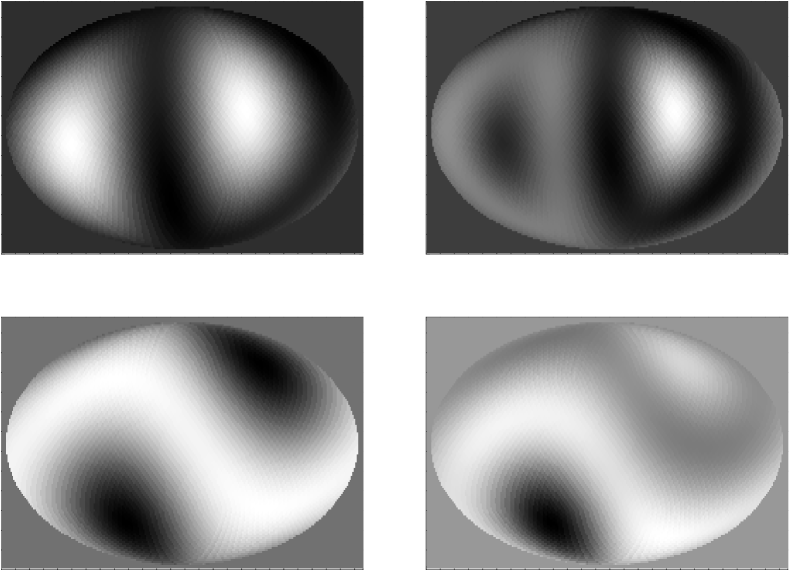
Figure 8: Two examples of a quadrupole (left) and octopole (right) realizations of a random sky that have particularly high value of the $I$ parameter.

Figure 9: The probability distribution for the $I$ parameter for the ILC, Wd and Vdfs cases respectively. The thin line corresponds to the prior distribution, while the thick line to the distribution upon the addition of the data. The most likely point is normalized to one.

IV.3 Feature matching

As a third example of alignment statistic we present a new method for determining alignment of the quadrupole and octopole. If the two are aligned, one expects that hot-spots and cold-spots match between the two. We thus examine the cross-correlation map created by multiplying the quadrupole and octopole maps:

$$T_{\times}=\hat{T}_{\ell=2}\times\hat{T}_{\ell=3}.$$ (18)

These maps are created by first normalizing $a_{\ell m}$ so that $\mathsf{D}_{2}=1$ and $\mathsf{D}_{3}=1$ (this is indicated by hats in the above equation). We do this, because we want to decouple the multipole amplitude from the alignment effect. The integral of this map across the sky necessarily gives zero due to the orthogonality condition:

$$\int T_{\times}{\rm d}A=0.$$ (19)

However, the integral of the cross-correlation map gives a non-zero result

$$I=\int\left(T_{\times}^{2}\right){\rm d}A,$$ (20)

which is particularly high if the cold-spots and hot-spots match between the two. This is illustrated in Figure 8 where we show two examples of a random sky realization with a particularly high value of the $I$ parameter. The figure indicates that the method indeed captures the heuristic idea of aligned quadrupole and octopole in terms of hot and cold spot overlap.

We calculate the value of $I$ parameter for all three cases and also a large number (150000) of Monte Carlo simulations of a random sky to determine the prior distribution of the $I$ parameter. The results are shown in Figure 9. The value for the $I$ parameter in the case of the ILC map is again very high, with the random probability of being of that value or higher of only 0.9%. Once again this anomaly disappears in the case of the more conservative approaches, suggesting that the alignment is in the region most contaminated by the foregrounds.

IV.4 Alignment with the Ecliptic pole

As a final example of the application of our method we investigate the asymmetry in the WMAP data on two hemispheres separated by the ecliptic plane. There were several reports of detection of this asymmetry using various methods Eriksen et al. (2003); Hansen et al. (2004a, b); Schwarz et al. (2004); Larson and Wandelt (2004). The method most relevant for us is the angle between multipole $\mathbf{w}$ vectors, defined in the Equation 17, and the ecliptic north pole Schwarz et al. (2004). This test is performed by calculating the dot product of the $\mathbf{w}^{\ell,i,j}$ vectors with the north ecliptic pole. We perform this multiplication for the quadrupole and call the resulting quantity $B_{2}$. When the same is performed for the octopole, we sort the values in ascending order and call them $B_{31}$, $B_{32}$ and $B_{33}$. Results of these analyses for our MCMC chains are shown in Figures 10 and 11.

We see that these results are considerably more stable with respect to the sky cuts and foreground marginalization than alignments discussed above. In order to asses this, we introduce three models:

• NULL model assumes that $B$ parameters are distributed according to the random sky hypothesis

• ALIGN1 model assumes that $B_{31}<0.02$ and $B_{32}<0.02$. This is effectively equivalent to the assumption that $B_{31}=B_{32}=0$, but with the advantage that its Bayesian evidence can be calculated from the existing chains.

• ALIGN2 model assumes $B_{31}<0.02$, $B_{32}<0.02$ and additionally $B_{2}<0.02$.

These models are, of course a posteriori. In fact, there are 16 possible models similar to ALIGN1 and ALIGN2 in which one or more $B$ are anomalously low. Therefore, interpretation of any result coming from the above should consider the the 1 in 16 factor coming from the biased choice of models. If we take into account the fact that one is working with the derived $\mathbf{w}$ vectors rather than the source multipole vectors $\mathbf{v}$ the biased choice “factor” becomes even higher.

Nevertheless, we asses the probability of this occurring by chance using two methods. Firstly, we measure the ratio of probabilities of each model given data to its probability in the isotropic case and secondly we calculate the Bayesian evidence for all three models for the Wd and Vdfs case. Bayesian evidence is the probability of a given model in the Bayesian context, assuming all models to have the same prior probability. It is the likelihood integrated over the prior volume and thus disfavors models that have either low likelihood or unnecessarily large number of parameters (leading to large volume of parameter space having low likelihood). For further discussion see MacKay (2002). See Appendix A for discussion of our method for estimating evidence. Results are shown in Table 3. The two methods are different in the way how the NULL model is treated (i.e. the $E_{\rm NULL}$ is sensitive to how well the data describe the isotropic model), but they nevertheless give similar results. While ILC does not show evidence for alignment as we defined it, the evidence for the alignment of the quadrupole and octopole planes with the ecliptic increases with the addition of the sky-cuts and foregrounds. This can happen if, for example, the real signal is contaminated by foregrounds, which destroy its evidence, but once the contamination is removed the signal comes out again. In Vdfs ALIGN1 model is 42 times more likely than the random model (which corresponds to $\sim 2.5\sigma$). As discussed above, however, once the biased nature of the models is taken into account, the real statistical significance is much smaller. The main point of interest here is that the alignment with ecliptic is less sensitive to foreground contamination than other alignments discussed above. We also calculated the dot product of the ecliptic north pole with the Angular Momentum Dispersion vectors, but the results did not show any evidence for alignment.

Figure 10: The probability distribution for the $B_{2}$ parameter. The prior distribution is flat. See Figure 11 for the distribution of the $B_{3i}$ parameters. The panels correspond to ILC (top), Wd (middle) and Vdfs (bottom).

Figure 11: The probability distribution functions for $B_{3i}$ (left to right) for the ILC (top), Wd (middle) and Vdfs (bottom) datasets. The most likely point is normalized to one.

Table 3: This table shows the two statistical tests used to asses the statistical evidence for ALIGN1 and ALIGN2 models as discussed in the text.

Dataset	$E_{\rm ALIGN1}/E_{\rm NULL}$	$\frac{p(\mbox{\tiny{ALIGN1}}|{\rm data})}{p({\mbox{\tiny ALIGN1}}|{\rm isotropic})}$	$E_{\rm ALIGN2}/E_{\rm NULL}$	$\frac{p(\mbox{\tiny{ALIGN2}}|{\rm data})}{p({\mbox{\tiny ALIGN2}}|{\rm isotropic})}$
ILC	$<10^{-3}$		$<10^{-3}$
Wd	$2.8\pm 0.04$	$4.3\pm 0.08$	$19.3\pm 1$	$19.0\pm 1$
Vdfs	$41.7\pm 0.2$	$63.9\pm 0.3$	$16\pm 1.2$	$15.6\pm 1$

V Conclusions

We developed a method to incorporate the uncertainties in the foreground removal and/or sky cuts into the statistical analyses that otherwise require a full sky data. Our method is based on deriving the full multi-dimensional likelihood distribution of the multipole moments given the data and the foreground uncertainties, noise or sky cuts. We compute this distribution using the MCMC sampling of the likelihood function, which is very fast, since we only need to invert the covariance matrix once. We recommend these methods are used to assess the statistical significance of an effect found in the full sky maps, to verify the sensitivity of the result to foreground uncertainties.

As an application of the method we have performed a detailed analysis of various quadrupole and octopole statistics in the WMAP data. For our standard procedure we use three datasets, ranging from the most aggressive (and probably contaminated) full sky ILC/TOH map to the V channel with applied KP2 mask and foreground marginalization of all three major contaminants, namely the Dust, Free-Free and Synchrotron emission. We used MCMC method to determine the probability distribution for the realization of the 12-dimensional quadrupole and octopole multipole moments.

We wish to emphasize again that probabilities of any a-posteriori statistic are always subjective (and some are more subjective than others, since they were more tailored for the data at hand). For this reason we focus here on the relative change in the probabilities between the least conservative ILC full sky map analysis and the most conservative map with galactic sky cut and foreground marginalization. The motivation is that if the probability changes strongly between these cases then it is not robust and may be contaminated by imperfect foreground removal in ILC/TOH map. This is of course not the only possibility: it is always possible that the data happen to contain important statistical information in the region most contaminated by the foregrounds. But our method provides some objective estimate of the probability for this to happen.

A point related to this is the question of how to formulate a statistically meaningful quantity that addresses various claims in the literature. For example, one could test perfect alignment between quadrupole and octupole ($d=1$), but a somewhat less perfect alignment could also be of potential significance as a sign of an anomaly. We address this by computing the integrated probability for a statistic to exceed a certain value and compare it to the random case. As the chosen value approaches the limit (e.g. $d=1$) the probability for the random case becomes very small, while if the data show signs of anomaly the integrated probability from the real data will remain significant. The ratio of the two thus gives some information on whether there is anything anomalous in the data.

We analyze the evidence for the low quadrupole and octopole. These are not particularly unlikely from ILC map, with the quadrupole probability being 3% and octopole being quite typical. These numbers do not change much by our more conservative treatment, so they appear robust. They are however significantly higher than the original values quoted by WMAP Spergel et al. (2003), which are statistically excluded and are therefore not a result of differences in foreground modeling. In a certain sense we have reached the opposite conclusion: from our analysis it appears impossible for the octopole to be anomalously low and the same is true for quadrupole in our Wd analysis. The difference may be a consequence of the noisier estimator used by WMAP.

We also discuss recent claims that the quadrupole and octopole are aligned. If one believes the ILC map, then the evidence for the quadrupole and octopole alignment is considerable. All three methods tested here, namely the maximum angular dispersion vectors, the multipole vectors and the feature matching method indicate that the two are suspiciously aligned. However, as soon as foreground uncertainties are included the evidence for this alignment disappears. It is not unexpected that the probability distributions broaden, but what is surprising is how rapidly the evidence vanishes and how strongly perfect or even partial alignment is excluded by the data. This strongly suggests that much of the evidence of the alignment comes from the portion of the data most contaminated by the galactic foregrounds.

Plots shown in this paper indicate a considerable difference between Wd and Vdfs cases. It is interesting to explore whether this difference comes from the number of templates being marginalised over or whether they are due to different frequency channels being employed. To investigate this we repeat the analysis using W channel data and marginalise over all three templates. The results are very similar to the Wd case, indicating that the main difference is due to different channel being employed. This suggests there might be additional systematic effects that are not handled properly even by our more conservative treatment. One possibility is that either V or W channel MEM derived foreground maps are contaminated on the largest scales, or that there are systematic contaminations in CMB maps Schwarz et al. (2004). More work is needed to explore these various possibilities.

Finally, we also present an example where our method can enhance the statistical significance by removing the contamination which would otherwise mask the evidence. We show that for the alignment of multipole vectors with ecliptic plane the statistical significance is not lowered by the foreground uncertainties. Once again, the statistical significance of this effect is unclear, but at least it seems clear that it is not significantly affected by the foregrounds and may even be enhanced, once the foreground contamination is removed from the data.

Our method is statistical and relies on the foreground templates to be faithful representation of all components that contaminate the data. Systematic uncertainties in the foregrounds translate in systematic uncertainties in derived quantities. Although our method provides a statistical framework for assessing the statistical significance of various effects, the real improvement will come from better understanding and modelling of the foregrounds. This goal can be achieved using multi-frequency data combined with a better understanding of physical processes involved. In this case a less conservative treatment of the foregrounds may be possible. We have tried some of these examples in our tests. Analyzing the original V or W maps without sky cuts, but with foreground template marginalization, causes MCMC sampler not to converge, which is indicative of a complex likelihood in this case. Similarly, using sky cuts but with no foreground removal shows clear evidence of contamination and causes the quadrupole and octopole to increase significantly Slosar et al. (2004). Subtracting the WMAP recommended foregrounds and using $\lambda=1$ in equation II.1 gives results very similar to $\lambda=\infty$. Thus we believe our results reflect the current uncertainties in the foreground subtraction and suggest these may be responsible for many of the anomalies seen in the WMAP data on large scales.

Appendix A Evidence calculation

The Bayes equation for the posterior probability of set of parameters $\bm{\theta}$ given a data-vector $\mathbf{d}$ can be written as

$$P(\bm{\theta}|\mathbf{d})=\frac{P(\mathbf{d}|\bm{\theta})P(\bm{\theta})}{P(\mathbf{d})}$$ (21)

The denominator of the right hand side is the evidence. See MacKay (2002) for a discussion of the usage of evidence as a Bayesian tool for model selection. Since the posterior must integrate to unity, one can write

$$E=P(\mathbf{d})=\int_{\bm{\theta}}P(\mathbf{d}|\bm{\theta})P(\bm{\theta}),$$ (22)

i.e. the evidence is the likelihood integrated over all priors. Evidence for completely disjoint models is usually calculated by the thermodynamic integration during the burn-in phase of the MCMC sampling (see e.g. Hobson and McLachlan (2003)). When considered models are a subset of the most general model, it is possible to calculate the relative evidence from the MCMC samples of the most general model. We perform the integral of the Equation (22) in bins that are $0.02$ in size over $B_{2}$, $B_{31}$, $B_{32}$. The integral is thus performed by adding up the prior probability corresponding to each sample. The prior probability is approximated to be constant over the entire bin. For the NULL model, the prior probability is obtained by binning the Monte Carlo simulations of random skies on the grid and normalizing. For the ALIGN1 and ALIGN2 models, the prior probability is one in the corresponding bin (i.e. $B_{31}<0.02$ and $B_{32}<0.02$ and zero otherwise). The prior probability for $B_{2}$ is constant at $0.02$ for models ALIGN1 and NULL. For the ALIGN2 it is one in the first bin and zero otherwise.

The error on the evidence are assumed to be only due to Poisson error in the number of samples in a given bin. If chains are well converged, this should indeed be the dominant error.

References

- Efstathiou (2003) G. Efstathiou, MNRAS 346, L26 (2003).
- Efstathiou (2004) G. Efstathiou, MNRAS 348, 885 (2004).
- Tegmark et al. (2003) M. Tegmark, A. de Oliveira-Costa, and A. J. Hamilton, Phys.Rev.D 68, 123523 (2003).
- Slosar et al. (2004) A. Slosar, U. Seljak, and A. Makarov (2004), eprint astro-ph/0403073.
- de Oliveira-Costa et al. (2004) A. de Oliveira-Costa, M. Tegmark, M. Zaldarriaga, and A. Hamilton, Phys.Rev.D 69, 63516+ (2004).
- Schwarz et al. (2004) D. J. Schwarz, G. D. Starkman, D. Huterer, and C. J. Copi (2004), eprint astro-ph/0403353.
- Eriksen et al. (2003) H. K. Eriksen, F. K. Hansen, A. J. Banday, K. M. Gorski, and P. B. Lilje (2003), eprint astro-ph/0307507.
- Eriksen et al. (2004) H. K. Eriksen, A. J. Banday, K. M. Gorski, and P. B. Lilje (2004), apJ, submitted, eprint astro-ph/0403098.
- Hansen et al. (2004a) F. K. Hansen, P. Cabella, D. Marinucci, and N. Vittorio (2004a), eprint astro-ph/0402396.
- Hansen et al. (2004b) F. K. Hansen, A. J. Banday, and K. M. Gorski (2004b), eprint astro-ph/0404206.
- Metropolis et al. (1953) N. Metropolis, A. W. Rosenbluth, M. N. Rosenbluth, A. H. Teller, and E. Teller, J. Chem. Phys. 21, 1087 (1953).
- Wandelt et al. (2003) B. D. Wandelt, D. L. Larson, and A. Lakshminarayanan (2003), eprint astro-ph/0310080.
- Wandelt (2004) B. D. Wandelt (2004), eprint astro-ph/0401623.
- Hivon et al. (2002) E. Hivon, K. M. Górski, C. B. Netterfield, B. P. Crill, S. Prunet, and F. Hansen, ApJ 567, 2 (2002).
- Tegmark (1997) M. Tegmark, Phys.Rev.D 55, 5895 (1997).
- Haslam et al. (1982) C. G. T. Haslam, H. Stoffel, C. J. Salter, and W. E. Wilson, A&AS 47, 1 (1982).
- Finkbeiner (2003) D. P. Finkbeiner, ApJS 146, 407 (2003).
- Finkbeiner et al. (1999) D. P. Finkbeiner, M. Davis, and D. J. Schlegel, ApJ 524, 867 (1999).
- Bennett et al. (2003) C. L. Bennett, M. Halpern, G. Hinshaw, N. Jarosik, A. Kogut, M. Limon, S. S. Meyer, L. Page, D. N. Spergel, G. S. Tucker, et al., ApJS 148, 1 (2003).
- Copi et al. (2003) C. J. Copi, D. Huterer, and G. D. Starkman (2003), eprint astro-ph/0310511.
- Larson and Wandelt (2004) D. L. Larson and B. D. Wandelt (2004), eprint astro-ph/0404037.
- MacKay (2002) J. C. D. MacKay, Information Theory, Inference and Learning Algorithms (Cambridge: Cambridge University Press, 2002).
- Spergel et al. (2003) D. N. Spergel, L. Verde, H. V. Peiris, E. Komatsu, M. R. Nolta, C. L. Bennett, M. Halpern, G. Hinshaw, N. Jarosik, A. Kogut, et al. (2003), eprint arXiv:astro-ph/0302209.
- Hobson and McLachlan (2003) M. P. Hobson and C. McLachlan, MNRAS 338, 765 (2003).