Chaos and the Effects of Planetary Migration on the Orbit of S/2000 S5 Kiviuq

Abstract

Among the many new irregular satellites that have been discovered in the last five years, at least six are in the so-called Kozai resonance. Due to solar perturbations, the argument of pericenter $\omega$ of a satellite usually precesses from 0 to $360^{\circ}$. However, at inclinations higher than $\simeq 39.3^{\circ}$ and lower than $\simeq 140.7^{\circ}$ a new kind of behavior occurs for which the argument of pericenter oscillates around $\pm 90^{\circ}$. In this work we will concentrate on the orbital history of the saturnian satellite S/2000 S5 Kiviuq, one of the satellites currently known to be in such resonance

Kiviuq’s orbit is very close to the separatrix of the Kozai resonance. Due to perturbations from the other jovian planets, it is expected that orbits near the Kozai separatrix may show significant chaotic behavior. This is important because chaotic diffusion may transfer orbits from libration to circulation, and vice versa. To identify chaotic orbits we used two well-known methods: the Frequency Analysis Method (Laskar 1990) and Maximum Lyapunov Exponents (Benettin et al. 1980). Our results show that the Kozai resonance is crossed by a web of secondary resonances, whose arguments involve combinations of the argument of pericenter, the argument of the Great Inequality ($2{\lambda}_{Jupiter}-5{\lambda}_{Saturn}$), longitude of the node $\Omega$, and other terms related to the secular frequencies $g_{5}$, $g_{6},$ and $s_{6}$. Many test orbits whose precession period is close to the period of the Great Inequality (883 yrs), or some of its harmonics, are trapped by these secondary resonances, and show significant chaotic behavior.

Because the Great-Inequality’s period is connected to the semimajor axes of Jupiter and Saturn, and because the positions of the jovian planets have likely changed since their formation (Malhotra 1995), the phase-space location of these secondary resonances should have been different in the past. By simulating the effect of planetary migration, we show that a mechanism of sweeping secondary resonances, similar to the one studied by Ferraz-Mello et al. (1998) for the asteroids in the 2:1 mean motion resonance with Jupiter, could significantly deplete a primordial population of Kozai resonators and push several circulators near the Kozai separatrix. This mechanism is not limited to Kiviuq’s region, and could have worked to destabilize any initial population of satellites in the Kozai resonance around Saturn and Jupiter.

1 Introduction

Carruba et al. (2002) studied an analytical model of the Kozai resonance (Kozai 1962) based on a secular development of the disturbing function, expanded in series of $a/a^{\prime}$ (where the ^′ stands hereafter for quantities related to the perturber), truncated at second order in $a/a^{\prime}$, and averaged over the mean anomalies of both perturber and perturbee (see also Innanen et al. 1997). Two kinds of behavior are possible in this simplified model: for inclinations of less than 39.23^∘ (or higher than 140.77^∘ for retrograde satellites), the argument of pericenter freely circulates from 0^∘ to 360^∘, while at intermediate inclinations a new class of solutions, in which the argument of pericenter librates around $\pm$90^∘, are possible. Such behavior is called the Kozai resonance. The value of the critical inclination of 39.23^∘ is, in fact, an artifact of the averaging; the real boundary between the region in which libration is possible or not is actually a more complicated function of the satellite’s semimajor axis and eccentricity (Ćuk et al. 2003, Ćuk and Burns 2004). Currently, six irregular satellites of jovian planets are known numerically to be in the Kozai secular resonance: two around Saturn (S/2000 S5 Kiviuq, and S/2000 S6 Ijiraq), two around Jupiter (S/2001 J10 Euporie, and S/2003 J20), and two around Neptune (S/2002 N2 and S/2002 N4, Holman et al. 2004). A third neptunian satellite, S/2003 N1 is on a chaotic orbit that may also be in the Kozai resonance (Holman et al. 2004).

A question that Carruba et al. left unanswered regarded the possible presence of chaos and chaotic diffusion at the separatrix between the regions of circulation and libration. Since in that work the authors considered a three-body problem, but averaged over the mean anomalies of both perturber and perturbee, our analytical model was an integrable one-degree of freedom model. In the real system, however, perturbations from other jovian planets and short-period terms may produce chaos near the Kozai separatrix. Chaotic evolution might lead to the escape of objects whose orbits were originally inside the Kozai resonance. Here we test the hypothesis that the chaotic layer is due to the fact that the Kozai resonance overlaps with secondary resonances near the separatrix. It is well known that resonance overlap is one of the major sources of chaos in dynamical systems (Chirikov 1979). Moreover, the positions of the planets may have changed after their formation, due to gravitational scattering of planetesimals (Malhotra 1995). As a consequence of the different planetary positions, the shape of the chaotic layer and the locations of the secondary resonances inside and outside the Kozai resonance should have been different in the past. This might have had consequences on the stability of any primordial population of Kozai resonators.

This paper will concentrate on identifying the chaotic layer at the transition between circulation and libration for Kozai resonators, in particular for the saturnian satellite Kiviuq, whose orbit is very close to the separatrix of the Kozai resonance. Our goal is to understand the origins of chaos and the effects of planetary migration.

Our investigation is divided in the following way: section 2 describes the major features of our simplified model of the Kozai resonance and identifies the transition region between circulation and libration. Section 3 recalls two methods to identify chaotic behavior in dynamical systems, the Frequency Analysis Method and the maximum Lyapunov exponents. Section 4 investigates possible causes of the chaotic layer. Section 5 shows how the Kozai resonance is crossed by a series of secondary resonances of different strengths. In the final section we demonstrate how the effect of planetary migration, combined with the effect of the secondary resonances, might have operated to depopulate a possible primordial satellite group of Kozai resonators.

2 Identifying the Transition between Circulation and Libration: Analytical and Numerical Tools

Carruba et al. (2002) described a simple analytical model of the Kozai resonance. This model is based on a development of the disturbing function in a series of $r/r^{\prime}$, where $r$ and $r^{\prime}$ are the radial planetocentric distances of the satellite and the Sun, truncated at the second order. The perturbing function $R$ is:

$$R=\frac{G_{0}m^{\prime}}{r^{\prime}}P_{2}(s)\left(\frac{r}{r^{\prime}}\right)^{2},$$ (1)

where $G_{0}$ is the gravitational constant, $m^{\prime}$ is the solar mass, $s$ is the angle between directions to the satellite and the Sun as seen from the planet, and $P_{2}$ is the second-order Legendre polynomial. The perturbing function, when averaged over the mean anomalies of both Sun and satellite, becomes:

$$R=\frac{G_{0}m^{\prime}a^{2}}{8b^{\prime 3}}\left[2+3e^{2}-\left(3+12e^{2}-15e^{2}{\cos^{2}{\omega}}\right){\sin^{2}{I}}\right],$$ (2)

where $a,e,$ and $I$ are the semimajor axis, eccentricity, and inclination of the satellite, respectively. $b^{\prime}=a^{\prime}\sqrt{1-e^{\prime 2}}$ is the Sun’s semiminor axis. The perturbing function, when expressed in terms of Delaunay elements ($l,g,h,L,G,H$; see Murray and Dermott 1999, Danby 1988), is:

$$R=-\frac{m^{\prime}L^{4}}{8b^{\prime 3}G_{0}m^{\prime}}\left[-10+\frac{3}{L^{2}}(3G^{2}-4H^{2})+\frac{15H^{2}}{G^{2}}+15{\cos^{2}{g}}\left(1-\frac{G^{2}}{L^{2}}-\frac{H^{2}}{G^{2}}+\frac{H^{2}}{L^{2}}\right)\right].$$ (3)

Since both $l$ and $h$ are cyclic, the conjugate quantities $L$ and $H$ are constants of the motion, as is the quantity:

$$\Theta=\left(1-e^{2}\right){\cos^{2}{I}}=H^{2}/L^{2}.$$ (4)

With $L$ and $H$ fixed, the perturbing function (3) represents a one-degree of freedom model for the Kozai resonance (Innanen et al. 1997). The following equations for the orbital elements hold:

$$\frac{dI}{d\tau} = -\frac{15}{16\sqrt{1-e^{2}}}\left(e^{2}\sin{2\omega}\sin{2I}\right),$$ (5)

$$\frac{de}{d\tau} = \frac{15}{8}e\sqrt{1-e^{2}}\sin{2\omega}~{}{\sin^{2}{I}},$$ (6)

$$\frac{d\omega}{d\tau} = \frac{3}{4\sqrt{1-e^{2}}}\left[2(1-e^{2})+5{\sin^{2}{\omega}}(e^{2}-{\sin^{2}{I}})\right],$$ (7)

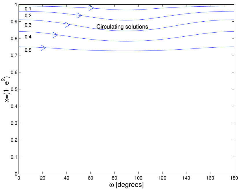
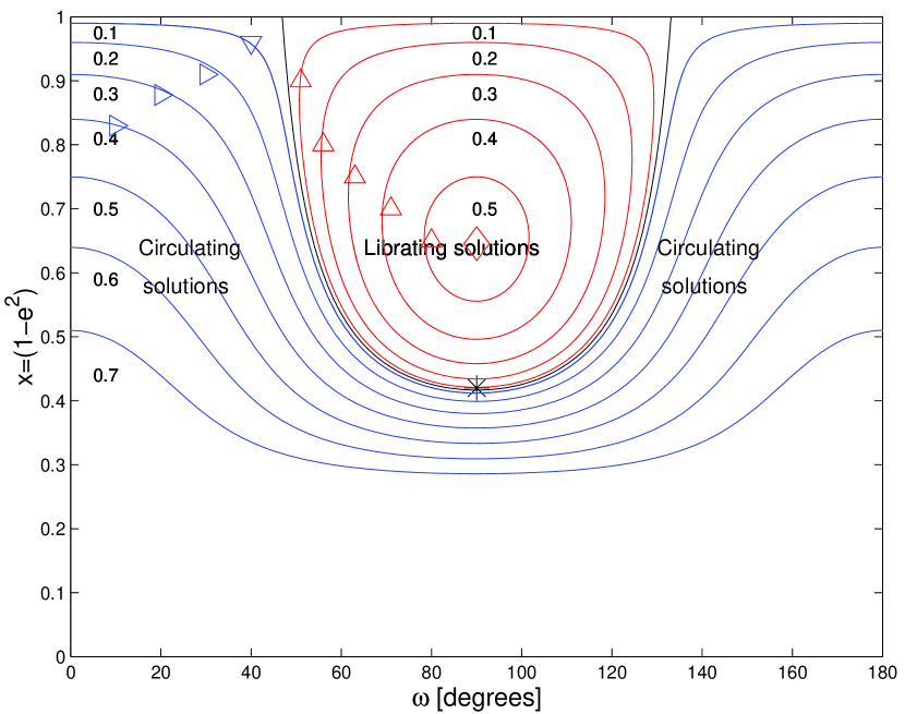
Figure 1: Energy levels of the Kozai Hamiltonian for $\Theta$ = 0.70 and = 0.25, in the $\omega$ vs. $1-e^{2}$ plane. Since the levels are symmetric about $\omega$ = $180^{\circ}$, we only show the interval $0-180^{\circ}$. For $\Theta<0.6$ librating solutions are possible (see the right panel).

where $\tau={G_{0}m^{\prime}t}/{nb^{\prime 3}}$ and t is time. The time has been rescaled in this way to eliminate the equations’ dependency on the satellite’s semimajor axis. Kinoshita and Nakai (1999) found the solution of (5-7) in terms of elliptic functions. Fig. 1 shows the results of numerical integrations of equations (5-7) for $\Theta=0.70$ and $\Theta=0.25$. For $\Theta$ less than 0.6, librating solutions are possible.

This model has several limitations. First, short-period terms have been eliminated by averaging. One consequence of this averaging is that the limit between the zones in which libration is possible or not is $I=39.23^{\circ}$ (or $140.77^{\circ}$ for retrograde orbits), regardless of the satellite’s semimajor axis (both inclinations correspond to $\Theta$ = 0.6 for $e=0$). When short-period terms are included, the boundary shifts slightly (Ćuk and Burns 2004). A case where this is observed is the orbit of the jovian satellite Euporie that is a Kozai resonator but has $\Theta>0.6$.

A second limitation of the averaged model is that, since it is an integrable, one-degree-of-freedom model, no chaos can appear at the separatrix between circulation and libration. Finally, since mutual perturbations among jovian planets are ignored, the orbital elements of the planet about which the satellites circle are constant. In the real solar system, the eccentricities of Jupiter and Saturn vary with several prominent periods associated with the secular frequencies $g_{5}$ and $g_{6}$ (timescales of up to $1/g_{5}\simeq 300,000$ yr), Great-Inequality terms $2\lambda_{J}-5\lambda_{S}$, where the suffices J and S hereafter stand for Jupiter and Saturn, (with a timescale of 883 yr), and short-period frequencies, connected with the orbital periods of the planets (12.5 and 29.7 yrs for Jupiter and Saturn, respectively). The shape of the separatrix may change in time according to the variations of the planet’s eccentricity and semimajor axis (remember the presence of the factor ${b^{\prime}}^{3}$ in $\tau$) which might introduce chaos along the real system’s separatrix.

To understand the behavior of the real system, we concentrate on the case of Kiviuq, a saturnian satellite in Kozai resonance whose orbit is very close to the separatrix between libration and circulation in $\omega$. We start by numerically searching for the transition between circulation and libration. To do so, we used the following procedure: we numerically integrated Kiviuq’s orbit over 100,000 yrs and found the maximum eccentricity, because then the satellite is closest to the separatrix. We computed $\Theta$ according to the inclination of Kiviuq at that time, and generated a grid of initial conditions for test particles; this contains 19 values in $\omega$, from $40^{\circ}$ to $140^{\circ}$, separated by $5^{\circ}$. All particles were given the average value of Kiviuq’s semimajor axis during the integration ($a=0.0755$ AU), and a grid in inclination with 21 values, starting at $38.6^{\circ}$ with a step of $0.6^{\circ}$. The values of the eccentricities were computed from $\Theta=0.4464$. Initial $\Omega$ and $M$ (mean anomaly) are equal to those of Kiviuq at its maximum eccentricity. This grid forms our “low-resolution survey”.

These initial orbits were integrated for 2 Myr under the influence of the four jovian planets (Outer Solar System, OSS hereafter) with a modified version of SWIFT-WHM, the integrator that uses the Wisdom and Holman (1991) mapping in the SWIFT package (Levison and Duncan 2000). We modified the integrator so that the planets’ orbits are integrated in the heliocentric system and the particles’ orbits are integrated in the planetocentric reference frame. This setup minimizes the integration error (Nesvorný et al. 2003).

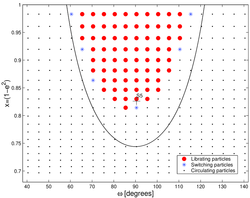
Figure 2: The fate of orbits located near the separatrix between circulation and libration for our low-resolution survey. Librating particles are shown by full dots, circulating orbits are shown by black points; and asterisks denote orbits that switched from libration to circulation. The black line identifies the separatrix according to the secular model for S/2000 S5 Kiviuq’s $\Theta$ at the maximum eccentricity. Kiviuq’s position is indicated by a cross (S5 in the figure).

To more easily identify secular oscillations in Saturn’s inclination, we refer all the positions to Saturn’s initial orbital plane. Fig. 2 shows the results of our simulations for our low-resolution survey. The actual separation between circulating and librating behavior does not follow the solution of the secular model when the full perturbations from jovian planets are considered. Moreover, some orbits alternate between circulation and libration (and, in a few cases, spend some time in the other libration island around $\omega=270^{\circ}$).

The question that remains to be answered is whether there is a chaotic layer near the separatrix, and if chaotic diffusion might be effective in depleting a primordial population of Kozai resonators. To address this question, and identify chaos, we will use the Frequency Analysis Method (FAM, hereafter; Laskar, 1990), and will compute the Maximum Lyapunov Exponents (MLE hereafter; Benettin et al., 1980) which we now describe.

3 Numerical Tools to Study Chaotic Orbits

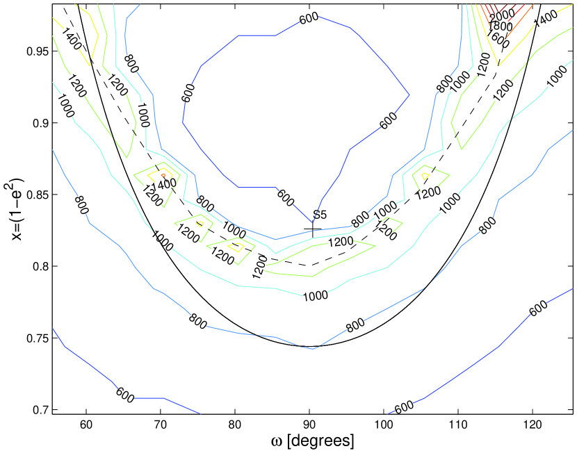
Figure 3: Contour plots that show the periods of libration or circulation in $\omega$ in years. The argument of pericenter $\omega$) lies on the horizontal axis, and on the vertical axis $x=1-e^{2}$. The solid parabolic line identifies the separatrix according to the secular model for S/2000 S5 Kiviuq’s $\Theta$ at the maximum eccentricity. The dashed line shows the approximate location of the actual separatrix (see Fig. 2).

The Frequency Analysis Method (FAM) is essentially an analysis of the frequency power spectrum of appropriate combinations of numerically determined orbital elements. In our case, for example, we are interested in the frequency related to the precession of the argument of the pericenter $\omega$. Fig. 3 shows the periods in $\omega$ for the particles in our low-resolution survey. The periods peak sharply in the transition region from circulation to libration in $\omega$, reaching a maximum of 1800 yrs. The minimum libration period is 480 yrs. The average period of libration in the Kozai resonance in our survey is 640 yrs. This range in periods corresponds to a frequency range of $\simeq$ 700-3200 “/yr.

We took the Fourier transform of $e\cdot\exp{\iota\omega}=e\cos{\omega}+\iota e\sin{\omega}$ (where $\iota=\sqrt{-1}$) over two time intervals (0-1 Myr and 1-2 Myr) and computed the quantity:

$$\sigma=\log{\left|1-\frac{f^{2}}{f^{1}}\right|},$$ (8)

where $f^{1}$ is the frequency over the first interval and $f^{2}$ the corresponding frequency on the second interval. If the motion is regular, $f(t)$ will be nearly constant, with small variations produced by errors in the determination of the frequencies (to be discussed later in this section). If the motion is chaotic, variations in $\sigma$ will be related to changes in $\omega$’s precession period.

While this is the main idea behind the FAM, a few complications occur. First, the precision of a Fast Fourier Transform (FFT hereafter) is limited by its coarse resolution [$\Delta f=\frac{1}{N\Delta\tau}$, where $\Delta\tau$ is the (constant) time separation of $\omega$-sampling and N is the number of data points used, which must be a power of 2 (Press et al. 1996)] in recovering the frequencies having the largest amplitude. To overcome this problem, we used the Frequency Modified Fourier Transform method (FMFT), with quadratic corrections (Šidlichovsky and Nesvorný 1997), which allows us to retrieve the frequencies with the largest amplitude to a better precision. To estimate the error associated with this method, we computed the frequencies with and without quadratic corrections, and computed the average value of the differences in $\sigma$. This procedure gives an upper limit on the error. In our case, the average error of FMFT was $\sigma=-4.5$, while a simple FFT had a resolution of $\sigma=-3$ (we used a time step $\Delta\tau$=30 yr, and 32,768 data points, so that each interval for the determination of the frequencies was $\simeq$ 1 Myr).

Another problem to take into account is aliasing. The FFT can recover frequencies up to the Nyquist frequency ($f_{N}=\frac{1}{2\Delta\tau}$, that corresponds to two samplings per period). Frequencies higher than the Nyquist frequency are not lost, but are mapped into a smaller apparent value of $f$, given by $f_{app}=f_{N}-(f_{real}-f_{N})$. This phenomenon is called aliasing and can be easily understood by considering a sinusoidal wave, sampled at isolated points: at least two points per period are needed to obtain a good estimate of the period . If the sampling is longer than one period, than the retrieved period is larger, and its “ghost” signature may appear in the frequency range of interest.

To avoid this problem, we used an “on-line” low-pass filter, following the procedure of Quinn et al. (1991) (based on the work of Carpino et al. 1987). Our filter suppresses to a level of $10^{-9}$ all Fourier terms with periods smaller than 66.7 yr (stop-band), and attenuates to a level of $10^{-9}$ all Fourier terms with periods between 66.7 and 200 yr. Terms with periods larger than 200 yrs are in the passband (see added information on website). By following this procedure, we have eliminated all frequencies connected with the orbital periods of Saturn and the satellites.

Finally, the shape of the frequency peaks can be modeled as Gaussian, but our measurements are made at isolated points. This introduces what in signal processing is called “impulse noise”, which can be attenuated by the use of a median filter (Press et al. 1996, Pitas 2000). More details about the use of the median filter and of the ${\chi}^{2}$ test we devised to prove the efficacy of our filter can be found in the Appendix.

To find an alternate way to distinguish between regular and chaotic behavior, we also computed Maximum Lyapunov Exponents (MLE) for our set of initial conditions. A detailed explanation of the theory of Lyapunov exponents goes beyond the scope of this paper; instead we refer the reader to Lyapunov (1907) and Benettin et al. (1980). MLE is a measure of exponential stretching of nearby orbits. The Lyapunov exponents are equal to zero for regular orbits (they tend to zero in finite-time calculations), while they assume positive values for chaotic orbits. The inverse of a Lyapunov exponent is the Lyapunov time $T_{L}$. Smaller values of $T_{L}$ indicate enhanced local stochasticity.

To estimate MLE for orbits we used a modified version of SWIFT-LYAP2, a code that integrates the difference equation (Morbidelli 2002) in the SWIFT package (Levison and Duncan 1994). The code was modified to reduce the integration error by integrating the planets in the heliocentric frame and the satellites in the planetocentric frame. For each of the test particles, we integrated the difference equation with an initial difference vector of modulus $d(0)=\sqrt{6}\cdot 10^{-9}$ and determined the modulus $d(t)$ of the displacement vector between the two vectors at time t. We constructed a series $[t,\ln{[d(t)/d(0)]}$ and performed a linear least-squares fit on this series. Since $d(t)\simeq d(0)\exp{(Lt)}$, where $L$ is the Lyapunov exponent, the slope of $\ln{[d(t)/d(0)]}$ versus time is equal to the Maximum Lyapunov exponent. We computed the Lyapunov exponents for all orbits in our low-resolution survey. We will show these results in the following section.

We should point out that FAM and MLE, while both useful tools to investigate chaotic behavior, measure different things. FAM measures macroscopic changes in frequencies (i.e., the speed at which chaotic motion changes the frequencies), while $T_{L}$ measures the rate of exponential stretching of nearby trajectories. These two techniques are complementary: FAM is more practical in finding regions that are macroscopically unstable, and $T_{L}$ can reveal the presence of different chaos-generating mechanisms. We will discuss in more detail these aspects of the two methods in the following section.

4 Origins of Chaos in the Kozai Resonance

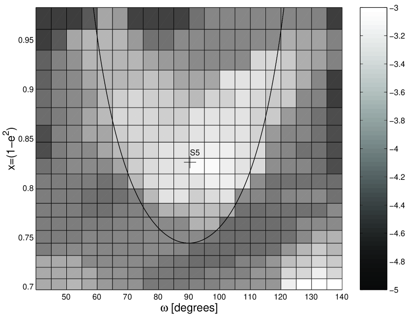
Figure 4: Low-resolution survey, grayscale plots of $\sigma$ values for $\Delta T$ =1 Myr. The solid parabolic arc in the figure’s center represents the separatrix according to the secular model (see Fig. 2). Chaotic orbits are associated with lighter shades (i.e., higher values of $log_{10}(\sigma)$, (see grayscale at right).

To investigate the presence of chaos, we applied the FAM to our low-resolution survey, integrated under the influence of the four jovian planets. Fig. 4 plots $\log{\sigma}$ for our low-resolution survey when the time interval between the first and the second frequencies was about 1 Myr. Fig. 4 shows that high values of $\sigma$ are found near the actual separatrix. The chaotic layer is asymmetric between values of $\omega>90^{\circ}$ versus $\omega<90^{\circ}$, and Kiviuq seems to be on the border of the chaotic layer.

Having shown that a chaotic layer exists, the next logical step is to ascertain its origin(s). Let us recall the analytical model presented in Section 2. In that model, the shape of the separatrix depends on Saturn’s semiminor axis $b^{\prime}$, which is a function of the semimajor axis and the eccentricity. Variations in Saturn’s semimajor axis and eccentricity may therefore generate complex orbital evolution near the separatrix. But on what time-scales? And how can we prove this hypothesis?

To study whether a variable $b^{\prime}$ may generate chaos, we performed a numerical simulation with the Sun (Saturn) on an orbit of fixed eccentricity (equal to the average value of the saturnian eccentricity) and the set of test particles used for our low-resolution survey. The difference compared to the integrable model is the presence of short-period terms. We performed the FAM on test orbits in our low-resolution survey and found that all orbits are regular in this case. In contrast, when only Saturn and the Sun were present, and Saturn had a constant eccentricity equal to the mean value computed during the 46,000 yr period of oscillation (= $1/g_{6}$), no chaos was observed. This seems to confirm our intuition that variations in Saturn’s eccentricity and semimajor axis may be responsible for the chaotic layer.

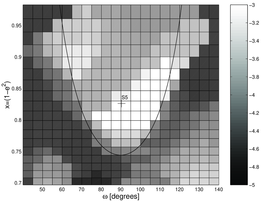
Figure 5: The level of chaos for a simulation where particles are subjected to the gravitational perturbations from Saturn and Jupiter. Chaotic orbits are in white, while orbits of regular behavior are in black (see grayscale at right).

To test this hypothesis, we performed a simulation in which both Saturn and Jupiter are present. In this case the layer of chaos appears (Fig. 5). The similarity between Figs. 4 and  5 suggest that the effects of Uranus and Neptune are unimportant. To demonstrate this, we performed two simulations with our low-resolution survey, one with the complete outer solar system (OSS), and the other with just Jupiter and Saturn. To show that the results are nearly equal we applied the ${\chi}^{2}$ test (see Appendix) to the filtered results of both simulations. We obtained a value of ${\chi}^{2}$ of 22.4 (out of a maximum number of 399) indicating a very high probability that the two distributions are the same. While perturbations from Uranus and Neptune might play a role in modifying the chaotic layer, such perturbations are clearly less important than Jovian perturbations. So, in the following, we only consider jovian perturbations. In doing so we of course modify the values of planetary frequencies and mean motions, and therefore the positions of any secondary resonances. But, since in this phase of our work we are interested in understanding on what timescales the chaotic behavior is driven, we believe this is an acceptable approximation.

There are two prominent timescales for oscillations of Saturn’s $e$ and $a$: the secular oscillations (period of order $1/g_{6}\simeq 46,000$ yrs) and the oscillations related to the Great Inequality (883 yrs). To study which of these perturbations is more relevant to the origin of chaos, we describe the OSS’ orbital evolution, in terms of Fourier series (Bretagnon and Francou 1988). In this model, the equinoctial orbital elements ($a,\lambda,K=e\cos{\varpi},H=e\sin{\varpi},Q=\sin{\frac{I}{2}}\cos{\Omega},P=\sin{\frac{I}{2}}\sin{\Omega}$) are developed in series of cosines and sines of combinations of twelve angles: four mean longitudes of the giant planets, four proper longitudes of pericenter, and four proper longitudes of the nodes. These proper angles are linear functions of time. This model assures a fractional precision better than $5\cdot 10^{-5}$ for $K,H,Q,$ and P over 10 Myr.

To investigate what minimal model can create a chaotic layer similar to the one observed in the full problem, we used different solutions for the orbits of both Jupiter and Saturn. We modified our version of SWIFT-WHM so that both orbital evolutions of Jupiter and Saturn are computed “on-line” according to the Bretagnon secular solution. The test particles are then subjected to perturbations of planets that evolve on such orbits. We considered four models for Saturn’s orbital evolution: (1) SEC, in which we limit the expansion to terms containing the $g_{5},g_{6},$ and $s_{6}$ frequencies for $K,H,Q,$ and $P$, assume a constant semimajor axis, and take 12 terms for $\lambda$’s development. (2) A21SEC, in which we have included 12 terms associated with the 1:2 commensurability between Jupiter’s and Saturn’s mean motions, and terms associated with the Great Inequality for the development in a, plus the same terms as in the SEC solution. (3) GISEC, in which there were 8 terms for $K$ and $H$, and 6 for $P$ and $Q$ associated with the Great Inequality, and a constant semimajor axis; and (4) A21GISEC, which includes the 2:1 terms in a, the Great-Inequality terms and the secular variations. Table 1 gives the number of terms taken in $a,\lambda,(K,H),(Q,P)$ for each solution.

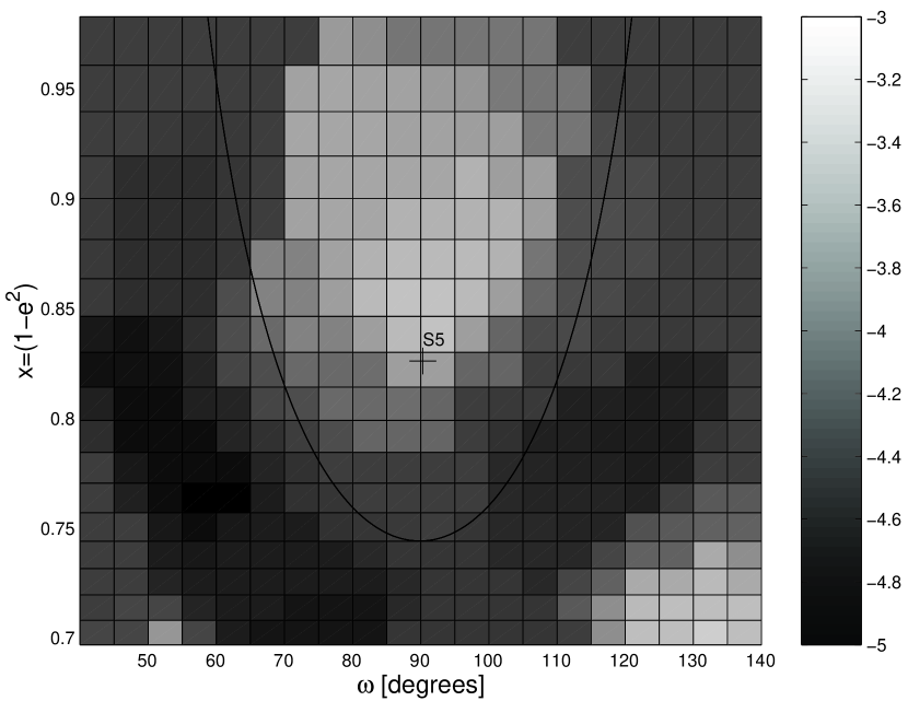
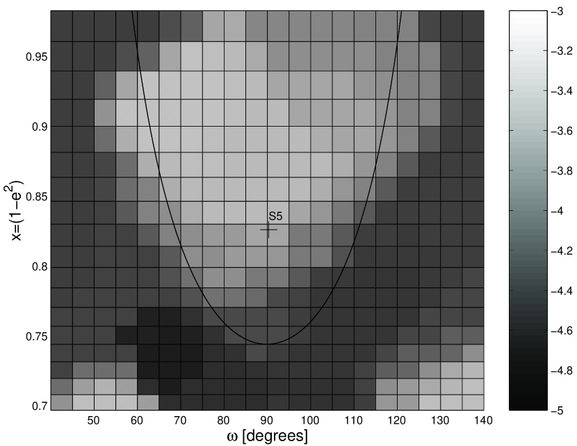
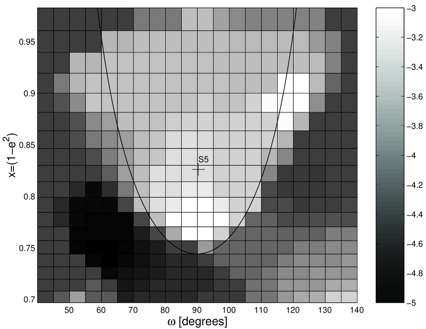
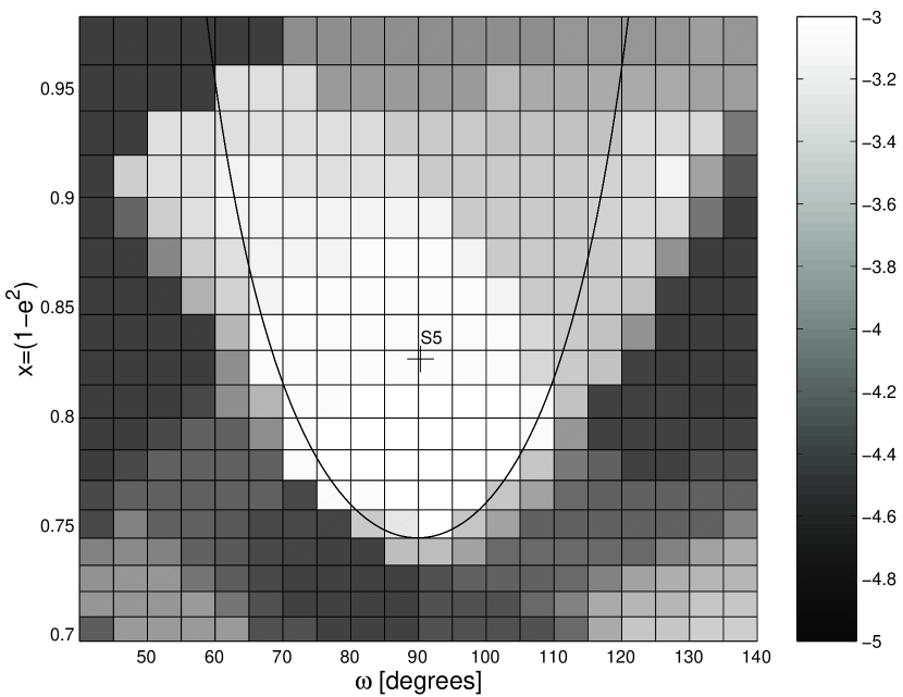
Figure 6: Measures of chaos for the simulation with the SEC Bretagnon solution (upper left), for the A21SEC Bretagnon solution (upper right), the GISEC solution (lower left), and the A21GISEC solution (lower right). Light shades correspond to $log_{10}({\sigma})=-3$ or to more chaotic orbits.

Fig. 6 shows the results of the integration with these models. All simulations used the same solution for Jupiter (10 terms in the development of $a$, 2 terms for $K$ and $H$, 2 for $Q$ and $P$, and 12 for $\lambda$). These figures may be compared with Fig. 5, where the traditional version of SWIFT-WHM was used.

Table 2 presents the results of a ${\chi}^{2}$ test in which we compared simulations with “Bretagnon” models with those of the full integration of Jupiter and Saturn. According to these results, terms associated with the Great Inequality and the 2:1 terms in the development of Saturn’s semimajor axis are the most important for the presence of the chaotic layer. The major sources for chaos are the variations in Saturn’s eccentricity connected with the Great Inequality.

To further investigate this hypothesis, we computed the maximum Lyapunov exponent for the particles of our low-resolution survey, in a model containing Jupiter and Saturn. Fig. 7 shows the resulting values of $T_{L}$ (left) when the full problem is considered and (right) when the planets evolve according to the SEC solution. A remarkable asset of Fig. 7a is the region of high values of $T_{L}$ (i.e., a smaller degree of local stochasticity) near the vertex of the separatrix, which, according to the FAM, is a region of high dispersion of the frequencies. In this region $T_{L}\approx 1,700$ yrs, i.e., twice the period of the Great Inequality; thus our results suggest that the feature is connected to a secondary resonance with the Great Inequality. Note, however, that all orbits seem to have quite small values of $T_{L}$. Orbits inside the libration island, which, according to FAM, are macroscopically regular, have $T_{L}<2,000$ yrs. This appears to be a general characteristic of high-inclination irregular satellite orbits, as all seem to have $T_{L}<10,000$ yrs (M. Holman, private communication, 2003).

The existence of a region characterized by relatively long Lyapunov times, on one hand, but high frequency dispersion, on the other, seems counter-intuitive at first. However, recall that the rate of frequency dispersion is a macroscopic characteristic of the orbit that is related to the global structure of the phase space region. In contrast, the Lyapunov time is a local property whose value is dictated by the mechanism that is responsible for the chaotic motion.

The existence of regions of large $T_{L}$ but rapid diffusion is not uncommon in the asteroid belt. For example, in the 7/3 resonance (see Tsiganis et al., 2003), the smaller values of $T_{L}$ are observed at the borders of the resonance where they are related to the pulsation of the separatrix due to secular precession. However, the macroscopically most unstable region is located at smaller libration amplitudes, is characterized by larger values of $T_{L}$, and is related to the colocation of the $\nu_{6}$ secular resonance. Similar results can be shown for other low-order mean-motion resonances (e.g., 2:1 and 3:1), where the most unstable zones are generated by coexisting secular resonances. As $T_{L}$’s value is typically of the order of the forcing period (e.g., $1/g_{5}\approx 305,000$ yrs, $1/g_{6}\approx 46,000$ yrs, Tsiganis and Morbidelli 2004), these regions generally have higher values of $T_{L}$ than the region associated with the pulsating separatrix of the mean-motion resonance.

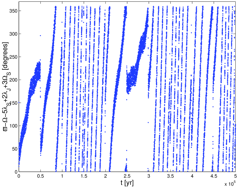
Figure 8: Time evolution of the angle $\varpi-\Omega-5{\lambda}_{S}+2{\lambda}_{J}+3{\Omega}_{S}$ for an orbit in the region of the secondary resonance involving the Great Inequality ($x_{0}=0.756,{\omega}_{0}=90^{\circ}$). Note how the resonant argument alternates between periods of libration and periods of circulation. This particle has a large value of $\sigma$.

We are likely observing a similar phenomenon in the case studied here. We believe that this high-$T_{L}$ region is associated with a secondary resonance, involving the Great-Inequality period. This is also supported by the results shown in Fig. 7b (SEC solution), where all orbits inside the libration zone become regular (note the different scale compared to Fig. 7a). To further support our claim, we selected a particle from this high-$T_{L}$ region, for which we plot the time evolution of the argument $\varpi-\Omega-5\lambda_{S}+2\lambda_{J}+3\Omega_{S}$ (Fig. 8). This corresponds to one of the possible critical arguments of the 1:1 resonance between the frequency of $\omega=\varpi-\Omega$ and the frequency of the Great Inequality, $2\lambda_{J}-5\lambda_{S}$ ($3\Omega_{S}$ is added in order to fulfill the d’ Alembert rules of permissible arguments, i.e., the sum of coefficients of individual longitudes must be zero and the sum of coefficients of nodal longitudes be even). The behavior of the arguments switches erratically between intervals of libration and circulation, which indicates a transition through the separatrix of this secondary resonance.

The following picture arises from our low-resolution surveys. Two major sources of chaos exist in the system. One is connected to the transition region from circulation to libration and, in particular, is driven by variations in Saturn’s eccentricity, mainly associated with Great-Inequality terms, and variations in Saturn’s semimajor axis. The other is related to a secondary resonance involving the argument of pericenter $\omega$ and the Great-Inequality terms for circulating particles. In most cases this resonance is a stronger source of chaos than the transition region. Better resolution is needed to understand the behavior and shape of this resonance (see Sec. 5).

One problem that remains to be explained is the asymmetry of the chaotic layer with respect to $\omega=90^{\circ}$ (see Figs. 5-7). According to the secular model, the result should be symmetric. Our simulations with the Bretagnon model suggest that variations in Saturn’s semimajor axis may be partly responsible for the asymmetry. Alternatively, the asymmetry in the chaotic layer may be related to our choice of initial conditions. To exclude this second possibility, we need to ascertain that our choice of initial conditions ($\Omega$ and $M$) for the test particles’ orbits is not introducing spurious effects. To our knowledge, three resonant configurations may alter the eccentricities of the test particles, and so put their orbits closer or farther away from the region of chaos that we are interested in. The three resonances are: ”nodal” ($\Omega-{\Omega}_{\odot}=$constant), pericentric ($\varpi-{\varpi}_{\odot}=0$), and the evection inequality [$2(\varpi-{\lambda}_{\odot})=$constant ($=45^{\circ}$, so as to have an intermediate value of the evection angle). In our simulation, the Sun’s orbit starts with: $\Omega=23.162^{\circ},\omega=311.992^{\circ}$, and $M=322.291^{\circ}$. We computed $\Omega$ for the test orbits according to the resonant configuration. For the pericentric resonance, we used two values of the resonant argument: $\varpi-{\varpi}_{\odot}=0$ and (Yokoyama et al., 2003), $\varpi-{\varpi}_{\odot}=180^{\circ}$, $\lambda-\lambda_{\odot}=180^{\circ}$. The second configuration maximizes the perturbing effect of the pericentric resonance.

To have a quantitative measure of the asymmetry, we use an “asymmetry coefficient” that is the difference of $\sigma$’s values for $\omega$ larger and smaller than $90^{\circ}$. To compute this coefficient for orbits in the libration island ($60^{\circ}<\omega<120^{\circ}$), we take two columns symmetric about $\omega=90^{\circ}$ (e.g., the columns for $\omega=60^{\circ}$ and $\omega=120^{\circ}$, with the obvious exclusion of the column for $\omega=90^{\circ}$) and compute the fractional difference for each pair. We repeat the process for all pairs of values and compute the average and standard deviation of the measurements. The average value is our “asymmetry coefficient”, and the standard deviation gives an estimate of the error. Obviously, the lower is the asymmetry coefficient, the more symmetric is the distribution of $\sigma$ around $\omega=90^{\circ}$.

Table 3 gives asymmetry coefficients for each simulation. Since the secular resonance with resonant argument equal to $0^{\circ}$ seems to give the more symmetric configuration, we believe its effect might be the dominant one (but large errors prevent our firm conclusion).

5 A Web of Secondary Resonance Crosses the Kozai Resonance

The low-resolution survey has yielded information regarding the large-scale structure of chaos inside the Kozai resonance. However, because most of the chaotic behavior is present near the boundary region between circulation and libration, we now concentrate on analyzing this region in more detail. For this purpose, we constructed a new set of initial conditions: we used 276 bins in inclination, starting at $37.5^{\circ}$ and separated by $0.02^{\circ}$. We used one $\omega$ (= $90.0^{\circ}$). The choice of the other orbital elements followed the same criteria used for the low-resolution survey. We called this new set of initial conditions a “high-resolution” survey. We concentrate on the region around $\omega=90^{\circ}$ to eliminate the problems associated with asymmetries in $\omega$ suggested by our low-resolution survey. Results of integrations of test particles with $\omega$ equal to $89.8^{\circ}$ or $90.2^{\circ}$ are very similar to those with $\omega=90^{\circ}$ and are not shown. Our choice of values for the particles’ inclinations allow us to sample periods in libration and circulation that go from a minimum of 450 yrs to a maximum of 820 yrs for librating particles, and from a minimum of 650 yrs to a maximum of 1820 yrs for circulating particles, thus covering the whole transition region.

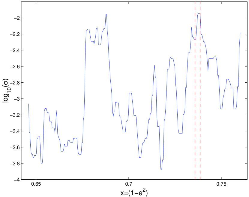
Figure 9: A plot of $log_{10}(\sigma)$ versus initial $x$ for our high-resolution survey. The dashed vertical lines show the transition region in which particles may switch behavior from circulation to libration. The two major sources of chaos for the system are this transition region and the pericentric secular resonance at $x$ = 0.68. Especially important in the context of planetary migration is the secondary resonance between $\omega$ and the Great Inequality at $x$ = 0.696. Other secondary resonances are also present.

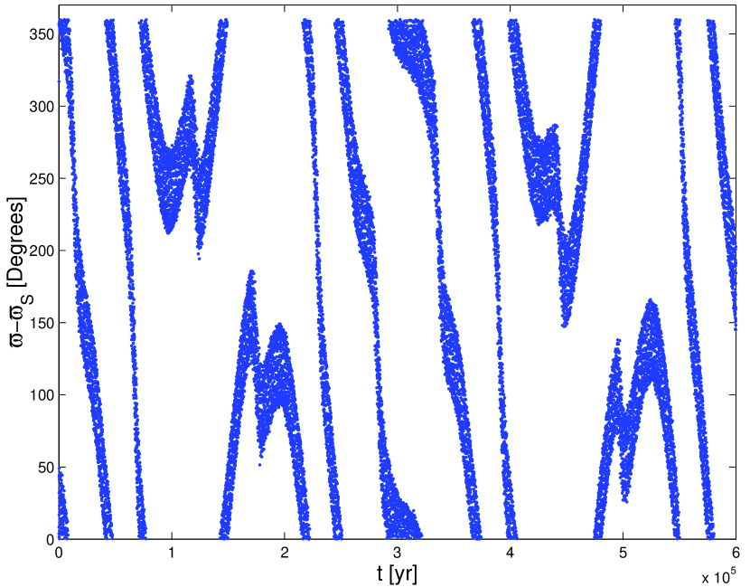
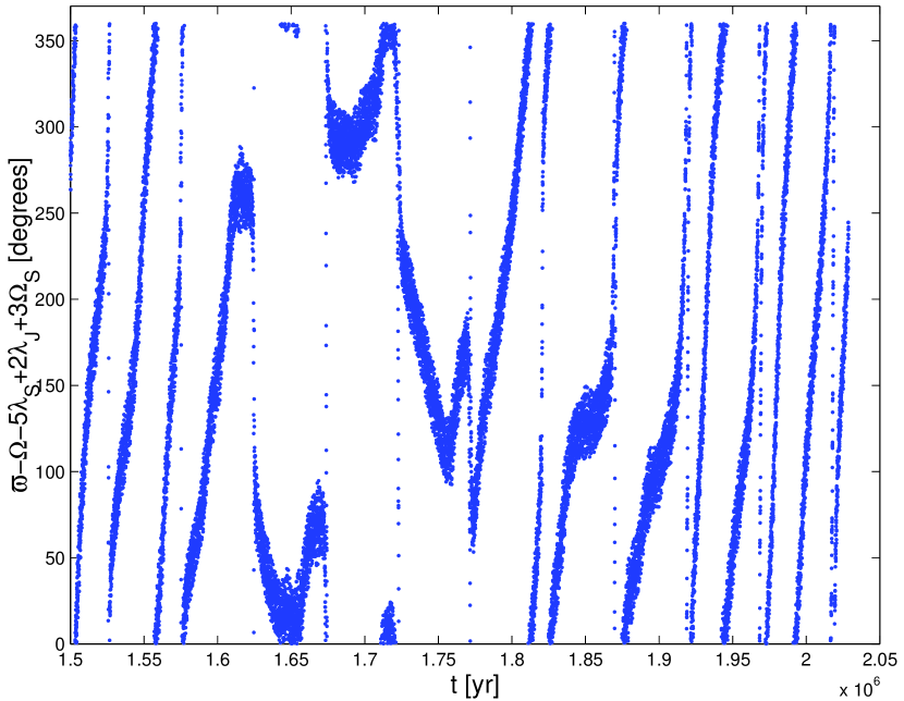
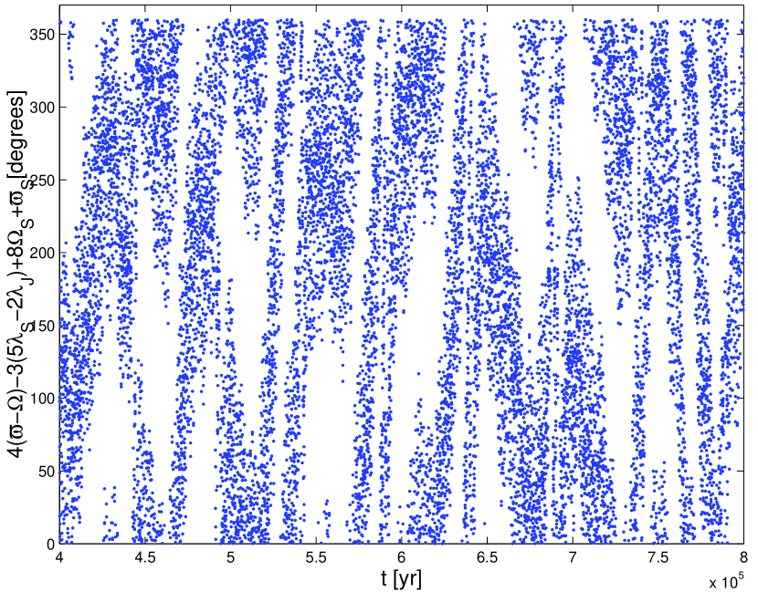
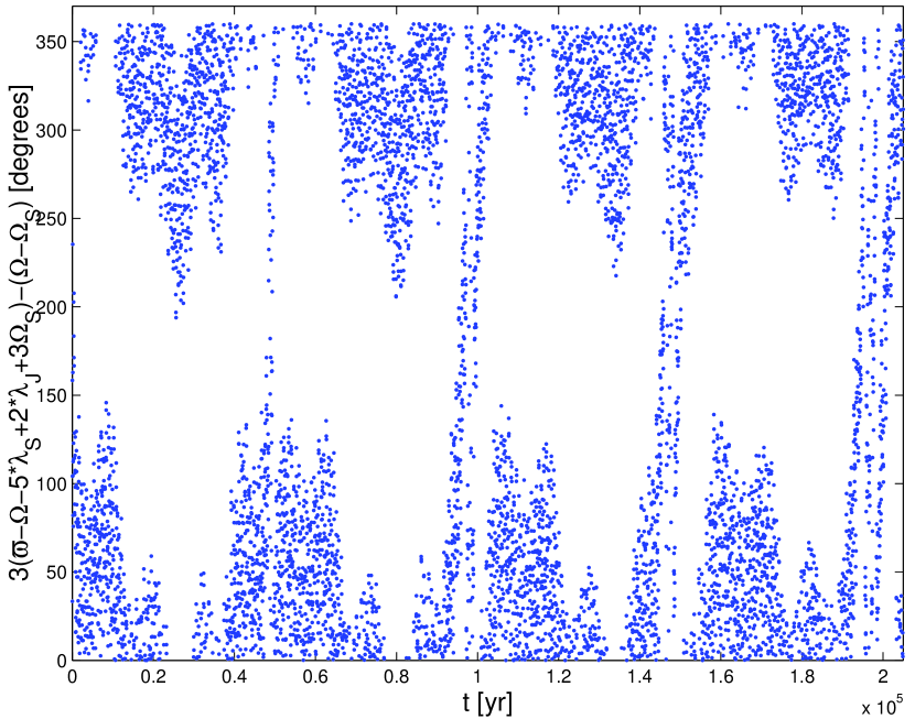
Figure 10: Resonant arguments for test particles in the a) pericentric secular resonance, b) resonance of argument $\varpi-\Omega-5\lambda_{S}+2\lambda_{J}+3\Omega_{S}$, c) resonance of argument $4(\varpi-\Omega)-3(5\lambda_{S}-2\lambda_{J})+8\Omega_{S}+\varpi_{S}$, and d) $3(\varpi-\Omega-5\lambda_{S}+2\lambda_{J}+3\Omega_{S})+(\Omega-\Omega_{S})$. All these particles shows periods of libration for their respective resonant angles. The orbital elements of planets and satellites are computed with respect to the solar system’s invariable plane.

We integrated the test particles of our high-resolution survey under the influence of the four jovian planets for 2 Myr and applied FAM. Fig. 9 shows two regions of high chaoticity. The one at $x\simeq 0.73$ is clearly associated with the transition from circulation to libration: test particles switch from $\omega$-circulation to $\omega$-libration at this $x$ (dots in the plot). The other region of strong chaotic behavior at $x\simeq 0.68$ is associated with the pericentric secular resonance ($\varpi-{\varpi}_{S}=0$). Fig. 10a shows the time evolution of the resonant argument for an orbit in this resonance ($x_{0}=0.6848$).

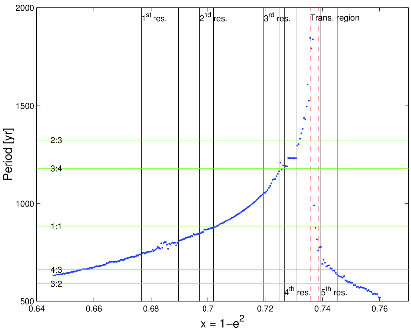
Figure 11: Periods of $\omega$’s precession obtained with FAM as a function of $x$. Vertical lines represent the locations of features of high $\sigma$, the dashed vertical lines show the transition region in which particles may switch behavior from circulation to libration, and the horizontal lines report the location of the commensurabilities between $\omega$ and the Great Inequality. The positions of the actual resonances slightly differ from that of the commensurabilities (see Eq. 9).

More interesting for our purposes is the region at $x\simeq 0.696$. A plot of the resonant argument $\varpi-\Omega-5\lambda_{S}+2\lambda_{J}+3\Omega_{S}$ shows that this feature is associated with the 1:1 resonance between $\omega$ and the Great Inequality (other resonances involving $\varpi_{S}$ and $\varpi_{J}$, instead of $\Omega_{S}$, are also present but are weaker. This property is generally shared by other resonances involving harmonics of the Great-Inequality period, like the 4:3, 3:2, etc.). The resonance we discovered is only present for circulating particles. A question that might arise is if a similar resonance could also be found for librating test particles. To answer this question we consider the periods of libration and circulation and estimate them by the frequency associated with $\omega$’s precession found via FAM. Fig. 11 shows such periods as a function of $x$. We also report the regions having high values of $\sigma$, possibly associated with secondary resonances (vertical lines), and the commensurabilities between periods in $\omega$ and Great-Inequality periods (for example, the 3:4 commensurability means that, for three periods in $\omega$ there are four periods in $2\lambda_{J}-5\lambda_{S})$.

We are conscious that the commensurabilities between the Great Inequality and $\omega$ are not real resonances, since they do not respect the d’ Alembert rules. Nevertheless, we think this is a useful plot, since gives a first-order estimate of the position of the real resonances. To compute the expected positions of the actual resonances we used the following procedure: for a resonance of argument $\varpi-\Omega-5\lambda_{S}+2\lambda_{J}+3\Omega_{S}$ (we will use $\omega$ for $\varpi-\Omega$ hereafter), the frequency of $\omega$’s precession for which there is resonant behavior is given by:

$$f_{\omega}=f_{GI}-3f_{s_{6}},$$ (9)

where $f_{GI}$ is the frequency associated with the Great Inequality term ($2\lambda_{J}-5\lambda_{S}$, equal to 1467.72 “/yr for the current position of the planets), $f_{s_{6}}$ is the frequency associated with $\Omega_{S}$ (= -26.345”/yr, Bretagnon and Francou 1988, the same source is used for the values of $g_{5}$ and $g_{6}$), and $f_{\omega}$ is the precession frequency. Analogous equations can be used for other resonances. From $\omega$’s frequency it is straightforward to determine the period of precession, and from that period we can determine the value of $x$. Fig. 11 seems to be very instructive. For example, since the period of the 1:1 resonance is 840 yrs and since the first test particle in librating regime has a period of 820 yrs, at the end of the transition region, there is currently no equivalent of the Great-Inequality secondary resonance for librating particles. Also, apart from the two regions with $\sigma$ associated with the pericentric secular resonance and the Great-Inequality resonance, another interesting feature of high chaotic behavior, which seems to be associated with a strong secondary resonance, appears at $x=0.73$. Fig. 11 shows how in this region the values of periods in $\omega$ are constant, which is an indication of librating behavior in a secondary resonance. Other regions of high $\sigma$ values can be found at $x=0.722$ and, in the librating region, at $x=0.741$ (since this region is so close to the separatrix, the chaotic behavior here observed might be related to the pulsating behavior of the separatrix itself, when perturbations from other jovian planets are considered).

We believe that the features of high $\sigma$ at $x=0.722$ and $x=0.73$ are associated with two other secondary resonances, whose resonant arguments are given by $4(\varpi-\Omega)-3(5\lambda_{S}-2\lambda_{J})+8\Omega_{S}+\varpi_{S}$ and $3(\varpi-\Omega-5\lambda_{S}+2\lambda_{J}+3\Omega_{S})+(\Omega-\Omega_{S})$, respectively. Fig. 10c and d show the behavior of the argument for orbits near these two resonances. Other weaker resonances connected with other commensurabilities between $\omega$ and $2\lambda_{J}-5\lambda_{S}$ are also observed. The resonance of argument $3(\varpi-\Omega)-2(5\lambda_{S}-2\lambda_{J})+5\Omega_{S}+\varpi_{S}$ is expected to be stronger than the one associated with the 3:4 commensurability, but its location is so close to the separatrix that its effect is difficult to discern. Table 4 lists the resonances for which the librating behavior of the resonant argument is observed, and a few candidates that could explain features of weaker chaos.

So far we have only discussed the case of circulating test particles. Features of weaker chaos, however, exist also in the librating region. Unfortunately, in this case plotting the resonant argument is not so easy, since, by the definition of libration, $\omega$ oscillates around $\pm 90^{\circ}$ instead of covering all values from $0$ to $360^{\circ}$. A possible way to overcome this problem would be to make a change of variables, so as to put the origin of the system of coordinates for $e\cos{\omega}$ and $e\sin{\omega}$ at the libration center. The new angle $\omega^{\prime}$ would then rotate from $0$ to $360^{\circ}$, and it would then be possible to check for the behavior of the resonant arguments by combining $\omega^{\prime}$ with GI and other terms. This procedure is rather cumbersome, especially since the libration point itself is not a fixed point, but, due to perturbations from the other jovian planets, oscillates with timescales associated with the Great Inequality, $g_{5},g_{6},s_{6}$, etc. Fortunately, there is an alternative method to determine whether a resonance has in its resonant argument terms associated with the Great Inequality.

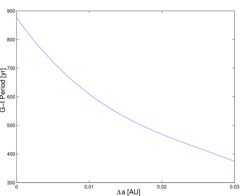
Figure 12: The period of the Great Inequality as it varies with positive expansions in Jupiter semimajor axis, assuming Saturn’s orbit fixed.

It is widely believed that planets have migrated since their formation (Malhotra 1995, Gomes 2003, Levison and Morbidelli 2003). In particular, the gravitational scattering of a planetesimal disk modified the positions of the jovian planets so that, while Saturn, Uranus and Neptune migrated outward in semimajor axis, Jupiter, being the most effective scatterer, migrated inward. As the work of Malhotra suggested, the origin of the highly eccentric, inclined, and Neptune-resonance-locked orbits of Pluto and the Plutinos might be explained in the context of sweeping resonant capture due to the changing position of Neptune’s orbit. Our work has shown that a major source of chaos for test particles in Kozai resonance around Saturn is due to a secondary resonance between the argument of pericenter $\omega$, the argument of the Great-Inequality (i.e., $2{\lambda}_{J}-5{\lambda}_{S}$), and terms connected with the planetary frequencies $g_{5},g_{6},$ and $s_{6}$. It is well known that by altering the positions of Jupiter and Saturn, the period of the Great Inequality changes. Fig. 12 shows how, by varying the initial value of the osculating semimajor axis of Jupiter by a positive amount (and keeping the position of Saturn fixed) it is possible to modify the period of the Great Inequality from the current value of 883 years to values of $\simeq 400$ yrs or less.

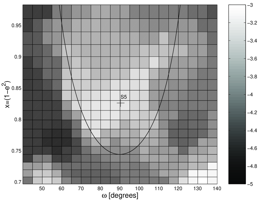
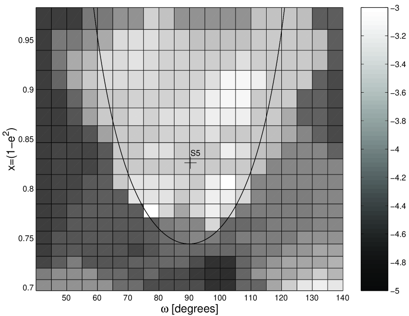
Figure 13: Shaded plots of $\sigma$ when the Great-Inequality’s period was (left) 640 yrs, and (right) 480 yrs. The position of the secondary resonance shifts upward toward the center of the libration island in the second case (480 yrs is the minimum period of libration).

The average and minimum values of $\omega$’s libration periods for particles in Kiviuq’s region are 640 yrs and 480 yrs, respectively. Presently, the Great-Inequality resonance has one location, just outside the separatrix, in the region of circulating particles. An interesting question would be to see what happened when the Great-Inequality resonance had a shorter period. In particular, when the value of the Great Inequality was shorter than $\simeq 820$ yrs (the maximum period of libration), a new secondary resonance should appear in the region of librating orbits. When the Great-Inequality’s period was 640 yrs, several particles in the libration island would have been in the region of this new secondary resonance. This can be seen in Fig. 13 which shows the results of the integration of our low-resolution survey integrated under the influence of Saturn and a Jupiter whose orbit was modified so that the period of the Great Inequality was a) 640 yrs, and b) 480 yrs. We called these simulations “static integrations”, as opposed to other simulations to be discussed in the next section for which the period of the Great Inequality is not fixed but changes with time. Note how the position of the high-chaoticity region, that our simulations show to be connected to the 1:1 resonance between $\omega$ and the Great Inequality, is displaced upward with respect to the traditional integration for the first case, and is very close to the center of the libration island for the second case. More important, a significant fraction (25%) of orbits that stayed inside the libration island in the integration with the present configuration of the planets were on switching orbits when the period of the Great Inequality was 640 yrs.

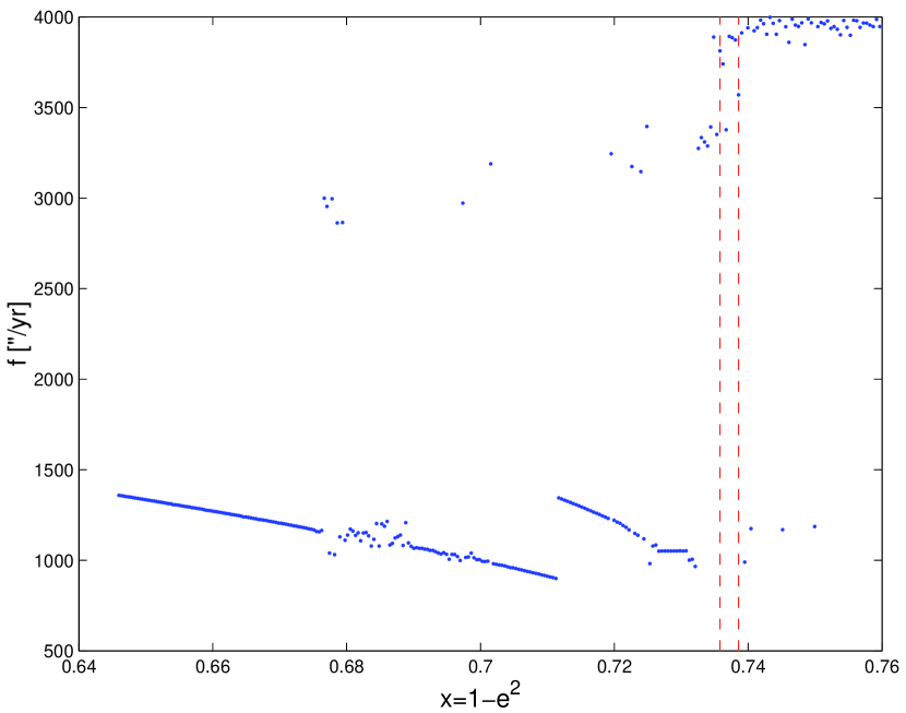
Figure 14: Variations in the frequency with largest amplitude as a function of $x$. When a resonance is encountered, frequency values are scattered ($x=0.68-0.69$). The curve is not continuous at $x=0.71$ because different frequencies have their largest values of amplitude for different regions in $x$. The dashed vertical lines show the location of the transition region, where orbits switch behavior from circulation to libration.

These simulations show that indeed a 1:1 resonance between $\omega$ and the GI (and the other terms needed to satisfy the d’Alembert rules) was present in the libration region when the GI’s period was lower. Coming back to our problem of identifying secondary resonances for the high-resolution survey, the method applied to our low-resolution survey to change the GI’s period can give precious insights on the identity of those resonances. Fig. 14 shows how the frequency with largest amplitude in the spectra obtained with FAM (just the frequency with largest amplitude, not necessarily the frequency associated with $\omega$’s precession) for our high-resolution survey changes with $x$. When a secondary resonance is encountered, values of the frequencies spread around rather than following a quasi-linear behavior (the feature associated with the pericentric secular resonance at $x=0.68$ is most instructive).

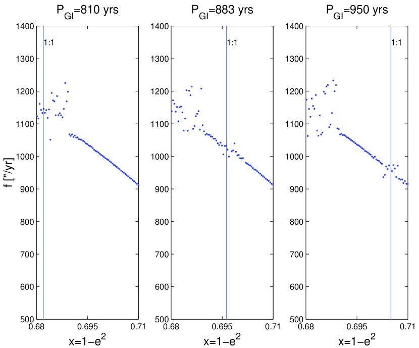
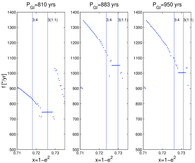
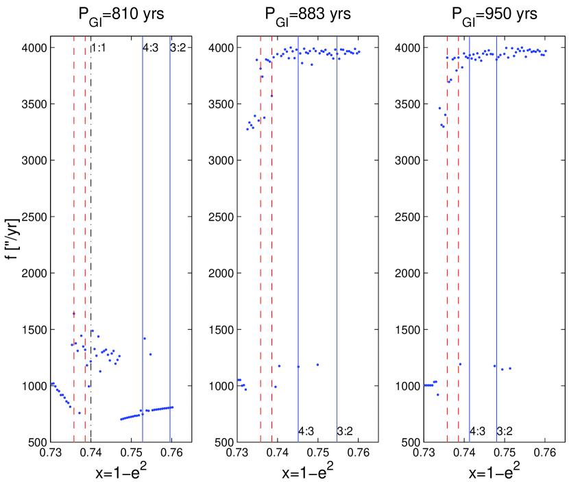
Figure 15: Variations in the frequency having the largest amplitude as a function of $x$, for three regions in $x$, and three values of the Great-Inequality’s period (810, 883, and 950 yrs, respectively). The first row of figures reports the region around the 1:1 GI resonance, the second the region around the 3:4 and resonance, and the third the region of librating particles. Vertical lines show the expected position of the resonance (identified at the top of the line) based on its resonant argument. By 3(1:1) we indicate the resonance of argument $3(\varpi-\Omega-5\lambda_{S}+2\lambda_{J}+3\Omega_{S})+(\Omega-\Omega_{S})$. Dashed vertical lines in the third row of figures show the position of the transition region. See text for more details.

To test our interpretation of the secondary resonances, we modified Jupiter’s position so that the GI period became 810, 883 (current value), and 950 yrs, respectively, and integrated the high-resolution survey with the three configurations. Figs. 15a, b, and c illustrate what happens to the frequencies for these three values of the GI, for the region of the 1:1 resonance, the 3:4, and for librating particles, respectively. Fig. 15a shows the behavior in the region of the 1:1 resonance. The resonance position (computed using Eq: 9 and the different GI periods) shifts toward larger $x$ when the GI period becomes longer. When the period equals 810 years, the position of the resonance corresponds to that of the pericentric secular resonance (note how its position does not move when the GI period is changed), and it goes to higher values of $x$ when we increase the period. The vertical lines indicate the expected position of the resonance when the GI period is modified. The fact that there is an excellent agreement between the predicted position of the resonance and the results of our numerical simulation seems to further confirm our hypothesis for the source of chaos in this region.

The middle row of Fig. 15 shows the same plots, but for $x=0.71-0.735$. This region contains two resonances of argument $4(\varpi-\Omega)-3(5\lambda_{S}-2\lambda_{J})+8\Omega_{S}+\varpi_{S}$, and $3(\varpi-\Omega-5\lambda_{S}+2\lambda_{J}+3\Omega_{S})+(\Omega-\Omega_{S})$: these are given the short-hand notation of 4:3 and 3(1:1). Once again, the numerical simulations demonstrate that the chaos zones move with the resonances, i.e., they agree with the predictions based on our resonant arguments (vertical lines).

Finally, the bottom row of Fig. 15 shows the values of the frequencies of largest amplitude for the region of librating satellites. The dashed vertical lines represents the transition region in which particles alternate from circulating to librating behavior. The left panel shows substantial frequency diffusion near the separatrix, when $P_{GI}=810$ yrs, not observed for longer Great-Inequality periods. We believe that this is due to the appearance of the 1:1 resonance (having argument $\varpi-\Omega-5\lambda_{S}+2\lambda_{J}+3\Omega_{S}$) in the region of librating particles (see the vertical line on the plot). This resonance is simply out of the range of periods in $\omega$ for librating particles when $P_{GI}>820$ yrs.

Regarding other resonances in the region, we are still limited by the problem of plotting the resonant argument. However, our simulations suggest at least two other resonances in this region: $2(\varpi-\Omega)-3(5\lambda_{S}-2\lambda_{J})+8\Omega_{S}+\varpi_{S}$ and $3(\varpi-\Omega)+4(5\lambda_{S}-2\lambda_{J})+11\Omega_{S}+\varpi_{S}$. The bottom row of Fig. 15 shows how the expected positions of these resonances shift when the Great-Inequality period is modified. In each case, the expected position is very close to regions of frequency variation. We believe this is strong circumstantial evidence in favor of the existence of these resonances. Other resonances containing combinations of only $\varpi_{J}$ or $\varpi_{S}$ instead of $\Omega_{S}$ (plus any other term needed to satisfy the second d’Alembert rule) in their argument are also possible, but, as observed in other cases, are associated with features of weaker chaos (their locations are not shown in Fig. 15). Regarding the bottom row of Fig. 15, we observe that the resonance positions shift toward the separatrix as the GI period increases.

To conclude, we have identified several secondary resonances connected to the Great Inequality for the region near the separatrix of the Kozai resonance. The likelihood that the jovian planets had different past positions means that the locations of these resonances might have also been different. This introduces interesting new prospectives for the stability of primordial satellites inside the Kozai resonance, that we now investigate.

6 Effects of Planetary Migration on Any Primordial Population of Satellites in the Kozai Resonance

We have just argued that a web of secondary resonances involving $\omega$, the argument of the Great Inequality, and other terms exists in the region of phase space around the separatrix between libration and circulation. Considering that the period of the Great Inequality might have been different in the past, we ask ourselves if a mechanism of sweeping secondary resonances inside the Kozai resonance, not dissimilar from the one that acted in the Kuiper Belt, could also have acted inside the Kozai resonance. If that is the case, what are the repercussions for the stability of satellites’ orbits in the Kozai resonance?

To address these questions we need to a) have a model of planetary migration and b) have an integrator able to simulate the effect of planetary migration for Jupiter and Saturn. Following Malhotra (1995), we assumed that the semimajor axis varied as:

$$a(t)=a_{f}-\Delta a\exp{(-t/\tau)},$$ (10)

where $a_{f}$ is the semimajor axis at the current epoch, $\Delta a$ is the change in semimajor axis (equal to -0.2 AU for Jupiter and to 0.8 AU for Saturn) and $\tau$ (= $2\cdot 10^{6}$) is a characteristic timescale for migration. For the integrator to simulate planet migration, we followed this recipe. We modified SWIFT-WHM so that an additional drag-force was applied to each planet along the direction of orbital velocity (by the symbol $\overline{v}$ we identify an unit vector along the direction of orbital velocity). This produces an acceleration:

$$\Delta{\bf\dot{v}}=\frac{\bf{\overline{v}}}{\tau}\left(\sqrt{\frac{G_{0}M_{sun}}{a_{f}}}-\sqrt{\frac{G_{0}M_{sun}}{a_{i}}}\right)\exp{(-t/\tau)},$$ (11)

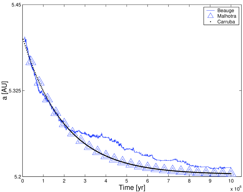
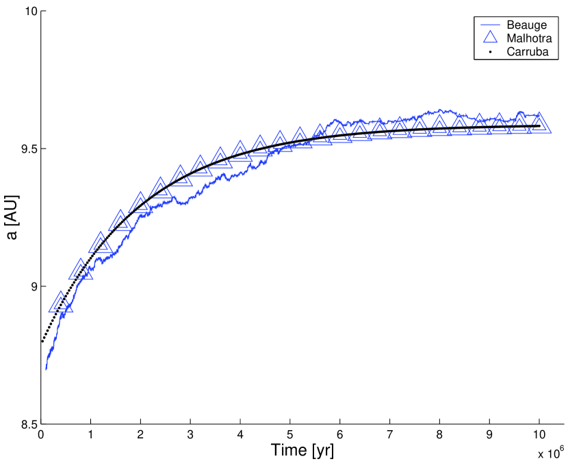
Figure 16: The time evolution of the semimajor axes of (left) Jupiter and (right) Saturn. The black band plots the results of our integrator, the triangles show the result of the integration of Eq. 10, and the line displays the results of a simulation on planetary migration from Beaugé et al. 2002, as described in the test.

where v̇ is the acceleration and $a_{i}$ is the initial position of a planet (Malhotra 1995). We neglected the effect of the planetesimals’ perturbations on the satellites. Fig. 16 displays several computed evolutions of Saturn’s and Jupiter’s semimajor axes. The two curves agree well. These are to be compared to the results of Beaugé et al. (2002) who used SWIFT-RMVS3 to simulate the evolution of a disk of 1000 massless planetesimals subjected to the gravitational perturbations of the four major outer planets. The evolution of the planet’s semimajor axes generally follows the exponential law of Eq. 10, but in addition is affected by short-time variations due to the impulses of single encounters.

Having now the tools for our investigation, we must define initial conditions for our simulations. To investigate the effect of planetary migration on the stability of orbits in the Kozai resonance, we first integrated Kiviuq with the integrator that accounts for planetary migration backward in time for 10 Myr. Not surprisingly, Kiviuq remained inside the Kozai resonance for the full length of the integration. We then used the last 100,000 yrs of the integration to compute the averaged orbital elements of Kiviuq and $\Theta$’s value (= 0.4322). Using this information, we generated a low-resolution survey of test particles, exactly as in Sec. 2. We then integrated this new set of initial conditions forward in time for 10 Myr. During this forward integration, the Great-Inequality’s period increased from 90 yrs at the beginning of the simulation to the current value of 883 yrs at the end of the integration.

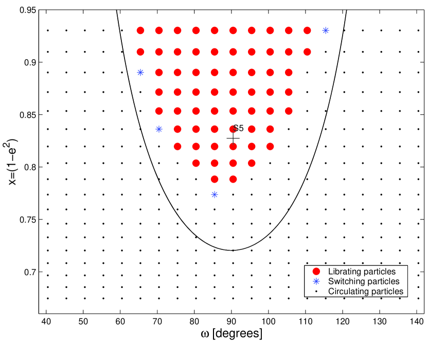
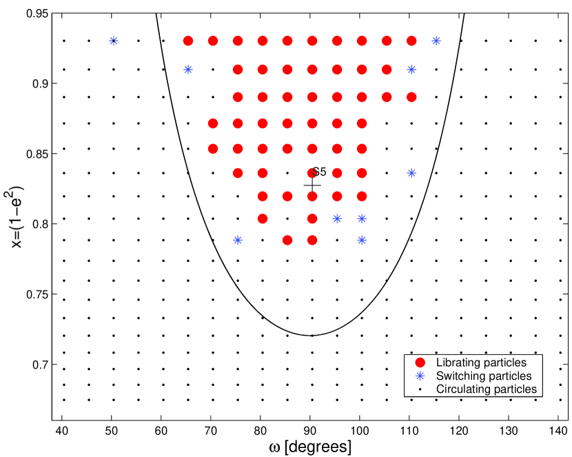
Figure 17: Fate of test particles for our low-resolution survey, where we used Eq. (10) to simulate planet migration. a) gives the orbital nature at the simulation’s beginning, while b) shows it at $t$ = 5 Myr; the symbols are the same used in Fig. 2. At the end of the simulation only one additional particle was lost from the libration island.

Fig. 17 shows the particles’ fates at left $t$ = 0 and right $t$ = 5 Myr. 14% of the particles originally in the libration island were on circulating or switching orbits by $t$ = 5 Myr. At the end of the simulation, 15% of the test particles originally in the libration island were no longer Kozai resonators. The mechanism of sweeping secondary resonances seems to be effective in depopulating the resonance. This mechanism not only affects orbits near the separatrix, but also those particles well inside the Kozai resonance. Examples are the particles with ${\omega}_{0}$ = $85^{\circ}$ and $x_{0}$ = 0.80 and 0.83, which are very close to Kiviuq’s orbital region. This shows that this region is also affected by the sweeping secondary resonances.

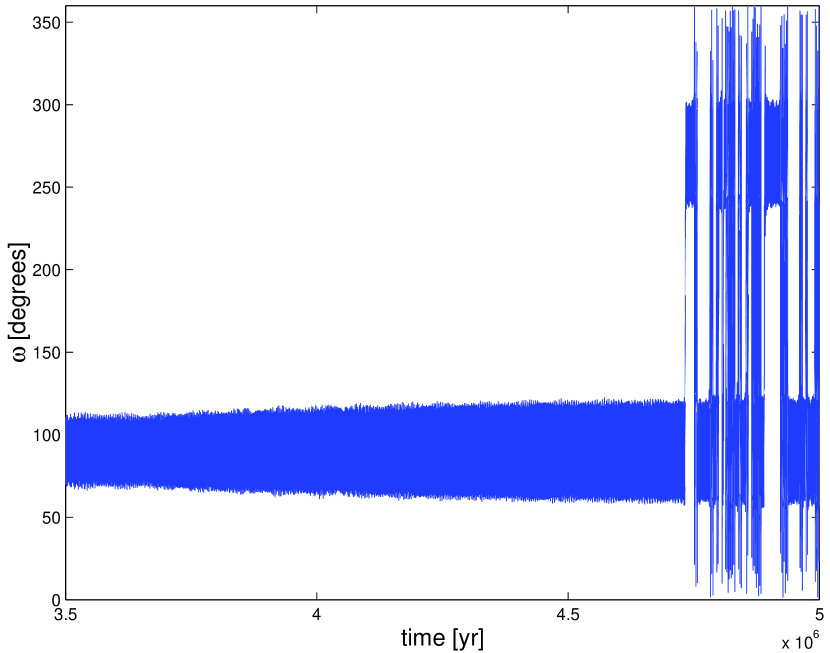
Figure 18: Time evolution of $\omega$ for an orbit initially inside the Kozai resonance ($x_{0}=83,{\omega}_{0}=85^{\circ}$). At $t=3.7$ Myr the particle is captured into the secondary resonance with the Great Inequality. As a consequence, the amplitude of libration slowly increases until the test particle reaches the separatrix of the Kozai resonance. At that point, it escapes from the resonance and starts switching back and forth from circulation to libration (around either $90^{\circ}$ or $270^{\circ}$). At the end of the integration ($t=10$ Myr) the particle was on a circulating orbit.

We explain these results in the following way: when, owing to the planets’ migration, the secondary resonance’s period approaches $\simeq 400$ yrs, a few of the particle inside the Kozai resonance (but only a fraction, the process is not 100% efficient) are captured into a secondary resonance, and move further out in the libration island until the secondary-resonance’s period attains $\simeq 700$ yrs. For such libration periods, the orbits are so close to the separatrix that escape becomes possible. This mechanism seems to be confirmed by the time evolution (Fig. 18) in $\omega$ for one of these particles ($x_{0}=0.83,{\omega}_{0}=85^{\circ}$).

The fact that most particles escape from the Kozai resonance in the first half of the simulation is not surprising. The period of the Great Inequality reaches 600 yrs during the first 5 Myr, i.e., the average value of the precession period for orbits in the Kozai resonance (see Fig. 3). After 5 Myr, the growing value of the Great-Inequality period sweeps fewer and fewer particles inside the Kozai resonance, and the mechanism loses its efficacy.

Another interesting consideration is that not only librating particles are pushed toward the separatrix, also some circulators in general are captured by one of the secondary resonances and are carried toward the separatrix. The fact that circulators do not generally become librators is due to the fact that in order to cross the separatrix they have to reach very high values of the precession period in $\omega$ (see Fig. 11). Once close to the separatrix, they reach a highly chaotic region, and many particles are lost from the secondary resonances. This mechanism could explain why so many irregular satellites are currently found in the proximity of the Kozai separatrix (Ćuk & Burns 2004 for AJ).

A word of caution should be given about our results. We only used a smooth exponential evolution (Malhotra 1995) for the planet’s migration. In the real Solar System things were most likely different from this model; e.g., Hahn and Malhotra (2000) introduced short-time scale variations in Neptune’s outward expansion by adding some random jitter to the torque applied to Neptune (cf. the $a$ history by Beaugé et al (2002) shown in Fig. 16). This jitter was parametrized by the standard deviation ${\sigma}_{jitter}$ of the planet-migration torque in units of the time-averaged torque. For small values of ${\sigma}_{jitter}$ ($<10$), capture efficiencies in the 2:1 resonances were substantially unaltered, and only when ${\sigma}_{jitter}$ reached values larger than 25 were capture probabilities reduced.

In our case, we can assume that a similar mechanism should be at work, and that any significant amount of short-time variations in the semimajor axes of both Jupiter and Saturn might in principle reduce the capture efficiency into the Great-Inequality secondary resonance. Since our work is, in many ways, exploratory, we believe the use of the exponential model is defensible at this stage of our study. But we acknowledge that a more realistic model for the motions of Jupiter’s and Saturn’s semimajor axes should be used, before realistic values of capture probabilities for our mechanism of sweeping secondary resonances could be computed.

In any case, we believe that our mechanism of sweeping secondary resonances might be an effective scheme for destabilizing the primordial population of bodies originally in the Kozai resonance. The mechanism should not be limited to Kiviuq’s region. The fact that the Great-Inequality’s period swept through values starting from 90 yrs at the beginning of the simulation with planetary migration to the current 883 yrs, implies that an analogous mechanism should also have been at work in the regions of the other Saturnian and Jovian satellites presently in the Kozai resonance, for $\omega$ libration periods of less than 1000 yrs.

7 Summary and Conclusions

We have analyzed the orbital behavior of satellites inside and outside the Kozai resonance for the phase space around the Saturnian satellite Kiviuq. Our goal was to identify areas of chaotic behavior and to understand if chaotic diffusion might have played an important role, now or in the past, for orbital stability inside the Kozai resonance. By applying the frequency analysis method (FAM) and computing the maximum Lyapunov exponents, we identified several secondary resonances. The major source of chaos for orbits in the circulating region are secondary resonances involving the argument of pericenter $\omega$ (= $\varpi-\Omega$), the Great-Inequality’s argument ($2{\lambda}_{J}-5{\lambda}_{S}$), the longitude of the node ($\Omega$), and the planetary secular frequencies ($g_{5},g_{6}$, and $s_{6}$). The region of transition between circulation and libration of $\omega$ is strongly chaotic, when perturbations from the other jovian planets are considered. According to our secular model, variations in Saturn’s semiminor axis (and, therefore in its eccentricity and semimajor axis) are what drive the chaotic behavior, especially the transfer from circulation to libration. While secular variations modulated by the $g_{5},g_{6},$ and $s_{6}$ frequencies are not negligible, once again our results indicate that the dominant effect is connected with perturbations having the Great-Inequality’s period.

Also, contrary to what might be expected from the secular model, our results indicate that the chaotic layer at the boundary between circulation and libration is not symmetric, but shows an asymmetry between values of $\omega$ larger and smaller than $90^{\circ}$. This is a consequence of other perturbations connected with secular pericentric resonance, evection inequality, and variations in Saturn’s semimajor axis, which are strongly dependent on the initial conditions for particles’ $\varpi$ and the Sun’s position. Our simulations suggest that the dominant effect is connected with the secular resonance, but variations in Saturn’s semimajor axis are not entirely negligible.

From our simulations we can introduce the following scenario for chaotic orbits near Kiviuq’s Kozai resonance. Starting from librating orbits close to the libration center, we possibly identify two weak secondary resonances of argument $2(\varpi-\Omega)-3(5\lambda_{S}-2\lambda_{J})+8\Omega_{S}+\varpi_{S}$ and $3(\varpi-\Omega)-4(5\lambda_{S}-2\lambda_{J})+11\Omega_{S}+\varpi_{S}$ that introduce chaotic behavior. The first strong source of chaos is however connected with the transition region between circulation and libration: orbits start to switch back and forth from circulation to libration and the whole region is characterized by high values of $\sigma$. Once in the circulating regime, a strong resonance of argument $3(\varpi-\Omega-5\lambda_{S}+2\lambda_{J}+3\Omega_{S})+(\Omega-\Omega_{S})$ appears at $x$ = 0.73. In addition to that, the dominant source of chaos, excluding the nearby pericentric secular resonance, is connected to a secondary resonance with the Great Inequality of argument $\varpi-\Omega-5\lambda_{S}+2\lambda_{J}+3\Omega_{S}$ (these orbits have argument-of-pericenter periods of order 840 yrs). Orbits in the region of this secondary resonance show some of the highest $\sigma$ values among the test particles we studied. Other secondary resonances connected with the Great Inequality are also observed.

The fact that the dominant source of chaos for orbits in Kiviuq’s region is connected with the Great-Inequality secondary resonance opens interesting perspectives. It is believed that jovian planets formed in different locations than their current ones, and then migrated by gravitationally scattering the primordial population of planetesimals (Malhotra 1995). The possibility that planets occupied different semimajor axes in the past has important repercussions, since the Great-Inequality’s period is connected with the osculating semimajor axes of Jupiter and Saturn. In particular, when the two planets were closer together, the period of the Great Inequality was shorter. We simulated this effect first by changing the position of Jupiter so that the Great-Inequality’s period was 640 yrs and 480 yrs, respectively (“static integrations”). These simulations showed that, indeed the position of the Great-Inequality’s secondary resonance shifted higher. A twin resonance for librating particles appeared when the Great-Inequality’s period equaled the average libration period (640 yrs), and the minimum (480 yrs) (this resonance is not visible today because the maximum period of libration inside the Kozai resonance is of $\simeq 820$ yrs). Then we fully integrated Jupiter and Saturn with an integrator that simulates planet migration according to the exponential law of Malhotra (1995).

Our results show that a mechanism of sweeping resonances, analogous to the one that operated in the Kuiper Belt (Malhotra 1995), or inside the 2:1 mean motion resonance with Jupiter (Ferraz-Mello et al. 1998) must have operated as well inside the Kozai resonance. Our simulations show that 15% of the satellites originally inside the Kozai resonance became circulators or exhibited switching behavior when planets acquired their final orbits. Indeed several particles were captured into the secondary resonance with the Great Inequality (or other secondary resonances) and, as a consequence, their amplitudes of oscillation in $\omega$ increased until the test particles reached the boundary between circulation and libration, where escape became possible. Several particles on circulating orbits were also pushed toward the separatrix by an analogous mechanism of sweeping secondary resonances (but none crossed the boundary to become a librator). We believe that a similar mechanism might have acted in the past also for the region of phase space associated with the other jovian satellites currently inside or near the Kozai resonance. This process could explain why so many irregular satellites are currently found near the Kozai separatrix (Ćuk and Burns 2004).

In this work we used several numerical tools. In a few cases, like for example the median filter for our FAM results, we introduced a technique, that, while employed in other fields (for example in remote-sensing and in the analysis of data from martian probes), was not, to our knowledge, used previously in celestial mechanics for reducing FAM results. Still on the technical side, we created new integrators to account for the Bretagnon solutions of the giant planets and to simulate planetary migration (Malhotra 1995). We believe these tools might be useful for other studies, not only for the irregular satellites of jovian planets.

Several questions remain that might be the subjects of future research. In this work we could not compute reliable capture probabilities for the Great-Inequality resonances when planetary migration is considered, since short-period variations in the semimajor axes of Jupiter and Saturn should also be taken into account (Hahn and Malhotra 2000, Beaugé et al. 2002). It would also be interesting to extend our studies to the neighborhoods of the other jovian satellites currently inside the Kozai resonance, and see if a web of secondary resonances (possibly involving the Lesser Inequality, the 2:1 quasi-resonance between Neptune and Uranus) is also present for the case of those neptunian satellites in Kozai resonance (Holman et al. 2004). We hope that this work might have opened interesting new prospects for the study of origins and stability of irregular satellites in Kozai resonance.

8 Acknowledgments

We are grateful to Thomas Loredo, Sylvio Ferraz-Mello, Richard Rand, Doug Hamilton, and Suniti Karunatillake for useful comments and suggestions supported in part by NASA’s Planetary Geology and Geophysics program. More information about this work is available at:

http://www.astro.cornell.edu/~valerio/FFT.

Appendix A Median filter and ${\chi}^{2}$ test

When measuring frequencies with a FMFT, the shape of the frequency peaks can be modeled as Gaussian, but our measurements are made at isolated points. This introduces what in signal processing is called “impulse noise”, which can be attenuated by the use of a median filter (Press et al. 1996, Pitas 2000).

In our case we took data on a running 3x3 matrix; the value at the central point is the median of the nine elements. Then we moved the matrix by one element and repeated the procedure. To compute values of $\sigma$ for points along the boundary of our figure, we added two external rows and columns of points all with values of $\sigma$ obtained from the average of all points in the figure. Once all elements were computed, we calculated the average of the percentage difference between the values of $\sigma$ before and after the median filter was applied. If the percentage difference was larger than 5$\%$, we repeated the procedure until convergence was assured. To test that our median filter is actually removing only noise and not actual data, we devised the following test. We applied our median filter to one of our low-resolution surveys, until the 5% convegence criterion was fulfilled. We then computed the difference ${\sigma}_{ij}$ between filtered ($F_{ij}$) and raw data ($R_{ij}$), and computed the standard deviation of the difference $\overline{\sigma}$. We then generated a fictitious matrix ${{\sigma}_{ij}}^{{}^{\prime}}$ of noise following a Gaussian distribution with standard deviation $\overline{\sigma}$ and zero mean, and added this fictitious noise to the filtered data, obtaining a matrix of $\sigma$ values $R_{ij}^{{}^{\prime}}$. The median filter was then reapplied to these new data until convergence was assured, and a new matrix $F_{ij}^{{}^{\prime}}$ obtained.

To compare the two distributions $F_{ij}$ of filtered data and $F_{ij}^{{}^{\prime}}$ (data obtained after the filtration of the fictitious noise), we devised the following scheme. We computed a ${\chi}^{2}$ variable, whose expression is given by:

$${\chi}^{2}={\Sigma}_{i}{\Sigma}_{j}\frac{({F_{ij}}^{{}^{\prime}}-F_{ij})^{2}}{{\sigma_{ij}}^{2}+{{{\sigma}_{ij}}^{{}^{\prime}}}^{2}},$$ (A1)

where $\sigma_{ij}$ and ${\sigma_{ij}}^{{}^{\prime}}$ are the errors on the values of the filtered data, intended as the difference between raw and filtered data. The variable so computed is supposed to follow a ${\chi}^{2}$ -like distribution. The problem is to determine the number of degrees of freedom of the distribution. This is not just given by the number (399) of data points in our low-resolution survey since, when taking the median, each value of $\sigma$ is connected to the value of at least some of its eight neighbors. Moreover, the process of filtering is applied several times, until convergence is assured, so that the number of degrees of freedom can be substantially smaller than the number of data points, in a way that is very difficult to estimate.

However, as a rule of thumb, a value of ${\chi}^{2}$ considerably smaller than 399 is a relatively good measure of a good fit. In the case of our test, the value of ${\chi}^{2}$ was 55, so we believe our test should be a convincing proof of the validity of our application of the median filter.

Figure 7: Lyapunov time for integrations (left) when the traditional version of the Lyapunov integrator is used and (right) when the SEC solution of the Bretagnon model is applied. The left figure has a feature of long Lyapunov times, associated with a region of high frequency dispersion, but on the right figure we see that this feature disappears when the SEC solution is used b). The substantially different gray scales used in the two figures were chosen to maximize the contrast between nearby features of $T_{L}$.

Table 1: The number of terms in $a,\lambda,(K,H),(P,Q)$ used for four separate solutions of Saturn’s orbit based on the Bretagnon model.

Model	$a$	$\lambda$	$(K,H)$	$(P,Q)$
SEC	1	12	2	2
A21SEC	12	12	2	2
GISEC	1	12	8	6
A21GISEC	12	12	8	6

Table 2: Results of a ${\chi}^{2}$ test that compares the filtered results of four Bretagnon simulations with the filtered results for a full simulation involving Saturn and Jupiter. Smaller values of ${\chi}^{2}$ indicates a better fit (the maximum number of degree of freedom is 399, see appendix). The models are described in the text.

Model	SEC	A21SEC	GISEC	A21GISEC
${\chi}^{2}$	2741.6	132.3	70.7	33.5

Table 3: Values of the asymmetry coefficient for four simulations with different initial conditions, corresponding to particles all having the same values of a) $\Omega-{\Omega}_{\odot}$ = constant, b) $\varpi-{\varpi}_{\odot}=0^{\circ}$, c) $\varpi-{\varpi}_{\odot}=180^{\circ}$, $\lambda-{\lambda}_{\odot}=180^{\circ}$, and d) $2(\varpi-{\lambda}_{\odot})=45^{\circ}$. Case b) seems to be the most symmetric, but all results overlap to within the errors.

Nodal Resonance	Pericentric Resonance	Pericentric Resonance	Evection Inequality
$\Omega-{\Omega}_{\odot}$ = const.	$\varpi-{\varpi}_{\odot}=0^{\circ}$	$\varpi-{\varpi}_{\odot}=180^{\circ}$	$2(\varpi-{\lambda}_{\odot})=45^{\circ}$
60$\pm$13%	55$\pm$12%	64$\pm$14%	60$\pm$18%

Table 4: Resonant arguments for the secondary resonances we observed or suppose to exist for the region near the separatrix of the Kozai resonance. The second column reports if the resonant argument was observed to librate. We used the word “suspected” or “strongly suspected” for resonances inside the libration region, whose positions, when the period of the Great Inequality was changed, moved according to our predictions. Other resonances involving higher commensurabilities between $\omega$ ($=\varpi-\Omega$) and the Great Inequality are weaker, and are not reported.

Resonant argument	Observed
$\varpi-\Omega-5\lambda_{S}+2\lambda_{J}+3\Omega_{S}$	yes
$\varpi-\Omega-5\lambda_{S}+2\lambda_{J}+2\varpi_{S}+\Omega_{S}$	yes
$\varpi-\Omega-5\lambda_{S}+2\lambda_{J}+2\varpi_{J}+\Omega_{S}$	no
$3(\varpi-\Omega)-2(5\lambda_{S}-2\lambda_{J})+5\Omega_{S}+\varpi_{S}$	no
$3(\varpi-\Omega)-2(5\lambda_{S}-2\lambda_{J})+5\varpi_{S}+\Omega_{S}$	no
$3(\varpi-\Omega)-2(5\lambda_{S}-2\lambda_{J})+5\varpi_{J}+\Omega_{S}$	no
$4(\varpi-\Omega)-3(5\lambda_{S}-2\lambda_{J})+8\Omega_{S}+\varpi_{S}$	yes
$4(\varpi-\Omega)-3(5\lambda_{S}-2\lambda_{J})+9\varpi_{S}$	yes
$4(\varpi-\Omega)-3(5\lambda_{S}-2\lambda_{J})+9\varpi_{J}$	no
$3(\varpi-\Omega-5\lambda_{S}+2\lambda_{J}+3\Omega_{S})+(\Omega-\Omega_{S})$	yes
$3(\varpi-\Omega-5\lambda_{S}+2\lambda_{J}+3\varpi_{S})+(\Omega-\varpi_{J})$	no
$3(\varpi-\Omega-5\lambda_{S}+2\lambda_{J}+3\varpi_{J})+(\Omega-\varpi_{S})$	no
$2(\varpi-\Omega)-3(5\lambda_{S}-2\lambda_{J})+8\Omega_{S}+\varpi_{S}$	strongly suspected
$2(\varpi-\Omega)-3(5\lambda_{S}-2\lambda_{J})+9\varpi_{S}$	suspected
$2(\varpi-\Omega)-3(5\lambda_{S}-2\lambda_{J})+9\varpi_{J}$	suspected
$3(\varpi-\Omega)-4(5\lambda_{S}-2\lambda_{J})+11\Omega_{S}+\varpi_{S}$	strongly suspected
$3(\varpi-\Omega)-4(5\lambda_{S}-2\lambda_{J})+11\varpi_{S}+\Omega_{S}$	suspected
$3(\varpi-\Omega)-4(5\lambda_{S}+2\lambda_{J})+11\varpi_{J}+\Omega_{S}$	suspected

References

- Beauge et al. (2002) Beaugé C., Roig F., and Nesvorný D. 2002, Icarus, 158, 483.
- Benettin et al. (1980) Benettin G., Galgani L., Giorgilli A. and Strelcyn J. M. 1980. Meccanica, March, 21.
- Bretagnon and Francou (1988) Bretagnon, P., and Francou, G., 1988, A&A, 202, 309.
- Carpino et al. (1987) Carpino, M., Milani, A., and Nobili, A. M. 1987, A&A,181, 182.
- Carruba et al. (2002) Carruba, V., Burns, J. A., Nicholson, P., and Gladman, B. 2002, Icarus, 158, 434.
- Chirikov (1979) Chirikov B. V. 1979, Physics Reports, 52, 265
- Ćuk et al. (2003) Ćuk, M., Burns, J. A., and Carruba V. 2003, Bull. Am. Astron. Soc., 35, 04.09.
- Ćuk and Burns (2004) Ćuk, M., and Burns, J. A. 2004, AJ, to be submitted.
- Danby (1988) Danby J. M. A. 1988, Fundamentals of Celestial Mechanics, 2nd ed,(Willmann-Bell, Richmond VA).
- Ferraz-Mello et al. (1998) Ferraz-Mello S., Michtchencko T. A., and Roig F. 1998, AJ, 116, 1491.
- Gomes (2003) Gomes R. S. 2003, Icarus, 161, 404.
- Hahn and Malhotra (2000) Hahn J.M, and Malhotra R. 2000, Bull. Am. Astron. Soc., 31, 01.10.
- Holman et al. (2004) Holman J. M., Kavelars JJ, Grav T., Gladman B. J., Fraser W., Milisavljiec D., Nicholson P. D., Burns J. A., Carruba V., Petit J. M., Rousselot P., Mousis O., Marsden B. G., Jacobson R. A. 2004, Nature, in press.
- Innanen (1997) Innanen K. A., Zheng J. Q., Mikkola S., and Valtonen M. J. 1997. AJ, 113, 1915.
- Kinoshita and Nakai (1999) Kinoshita, H. and Nakai, H., 1999, Celest. Mech. Dynam. Astron. 75, 125.
- Kozai (1962) Kozai Y. 1962, AJ, 67, 591
- Laskar, J. (1990) Laskar, J., 1990, Icarus 88, 266.
- Levison and Duncan (1994) Levison, H. F., and Duncan, M. J. 1994, Icarus, 108, 18.
- Levison and Duncan (2000) Levison, H. F., and Duncan, M. J. 2000, AJ, 120, 2117.
- Levison and Morbidelli (2003) Levison, H. F., and Morbidelli A. 2003, Nature, 426, 419.
- Lyapunov (1907) Lyapunov A. M. 1907, Ann. Fac. Sci. Univ. Toulouse, 9, 203.
- Malhotra (1995) Malhotra R. 1995, AJ, 110, 420.
- Morbidelli (2002) Morbidelli A. 2002, Modern Celestial Mechanics, 1st edition, (Taylor and Francis, London, UK).
- Murray and Dermott (1999) Murray C. D., and Dermott S. 1999, Solar System Dynamics, 1st edition, (Cambridge Univ. Press., Cambridge, UK).
- Nesvorny et al. (2002) Nesvorný, D., Alvarellos J. L. A., Dones, L. and Levison H. F. 2003, AJ, 126, 398.
- Pitas (2000) Pitas I. 2000, Digital Image Processing Algorithm and Applications, 1st edition, (J. Wiley, NY).
- Press et al. (1996) Press W. H., Teukolsky S. A., Vettering W. T., and Flannery B. P. 1996, Numerical Recipes in Fortran 77, 2nd edition,(Cambridge Univ. Press., Cambridge, UK).
- Quinn et al. (1991) Quinn, T. R. Tremaine, S., and Duncan, M., 1991, AJ, 101, 2287.
- Sidlichovský and Nesvorný (1997) Šidlichovský, M., and Nesvorný, D. 1997, Celest.Mech. Dynam. Astron. 65, 137.
- Tsiganis et al. (2003) Tsiganis K., Varvoglis H., and Morbidelli, A., 2003, Icarus, 166, 131.
- Tsiganis and Morbidelli (2003) Tsiganis K. and Morbidelli, A. 2003, NATO - ASI meeting ”Chaotic Worlds”, 2003.
- Yokoyama et al. (2003) Yokoyama, T., Santos, M. T., Cardin, G., Winter, O. C 2003, Astron. Astrophys., 401, 763.
- Wisdom and Holman (1991) Wisdom J., and Holman, M. 1991, AJ, 102, 1528