HYDRODYNAMICAL EFFECTS IN INTERNAL SHOCK
OF RELATIVISTIC OUTFLOWS

Abstract

We study both analytically and numerically hydrodynamical effects of two colliding shells, the simplified models of the internal shock in various relativistic outflows such as gamma-ray bursts and blazars. We pay particular attention to three interesting cases: a pair of shells with the same rest mass density (“equal rest mass density”), a pair of shells with the same rest mass (“equal mass”), and a pair of shells with the same bulk kinetic energy (“equal energy”) measured in the intersteller medium (ISM) frame. We find that the density profiles are significantly affected by the propagation of rarefaction waves. A split-feature appears at the contact discontinuity of two shells for the “equal mass” case, while no significant split appears for the “equal energy” and “equal rest mass density” cases. The shell spreading with a few ten percent of the speed of light is also shown as a notable aspect caused by rarefaction waves. The conversion efficiency of the bulk kinetic energy to internal one is numerically evaluated. The time evolutions of the efficiency show deviations from the widely-used inellastic two-point-mass-collision model.

1 INTRODUCTION

The internal shock scenario proposed by Rees (1978) is one of the most promising models to explain the observational feature of relativistic outflows as in gamma-ray bursts, and blazars (e.g., Rees & Meszaros 1992; Spada et al. 2001). In this scenario, the bulk kinetic energy of the outflowing plasma is converted into thermal energy and non-thermal particle energy by the shock dissipation and particle acceleration, respectively, and explain the large power of these objects. Based on this scenario, a lot of authors have attempted to link the observed temporal profiles to multiple internal interactions (e.g., Kobayashi, Piran, & Sari 1997 (hereafter KPS97); Panaitescu, Spada & Meszaros 1999; Tanihata et al. 2002; Nakar & Piran 2002 (hereafter NP02)), looking for crucial hints on the central engine of these relativistic outflows.

Most of the previous works focus on the comparison with the observed light curves and model predictions employing a simple inelastic collision of two point masses (KPS97) and little attention has been paid to hydrodynamical processes in the shell collision. However, it is obvious that, in the case of relativistic shocks, the time scales in which shock and rarefaction waves cross the shells are comparable to the dynamical time scale $\Delta^{{}^{\prime}}/c$, where $\Delta^{{}^{\prime}}$ is the shell width measured in the comoving frame of the shell and $c$ is the speed of light. Since the time scales of observations of these relativistic outflows (e.g., Takahashi et al. 2000 for blazar jet; Fishman & Meegan 1995 for GRBs) are much longer than the dynamical time scales, the light curves should contain the footprints of these hydrodynamical wave propagations. Thus, it is very interesting to clarify the difference between the simple two-point-mass-collision (hereafter two-mass-collision) model and the hydrodynamical treatment. The recent study by Kobayashi & Sari 2001 (hereafter KS01) reports that collided shells are reflected from each other by the thermal expansion. Since they perform a hydrodymamical simulation and show the reflection feature for a single case, the detail of propagations of rarefaction waves for various cases of collisions is not discussed. The aim of this paper is to clarify the hydrodynamical effects including the propagations of rarefaction wave. As the simplest case, we explore the hydrodynamics of two-shell-collisions in the internal shock model. Since we are mainly interested in the hydrodynamical processes themselves, it is beyond the scope of this paper to make a detailed comparison of the observed phenomena with the model results.

We consider the time evolution of two colliding shells in relativistic hydrodynamics in §2. In §3, we discuss the application to GRBs and blazars. The summary and discussion are given in §4.

2 HYDRODYNAMICS

Here we consider the hydrodynamics of the two-shell-interactions. Our intention is to derive analytically various time scales for shocks and rarefaction waves crossing the shells. The fundamentals of relativistic shocks are given by Landau & Lifshitz (1959) and Blandford & McKee (1976). Our main assumptions are (1) we adopt a planar 1D shock analysis and neglect radiative coolings for simplicity, (2) neglect the effect of magnetic fields, and (3)limit our attention to shells with relativistic speeds. We are currently planing 2D studies. The role of magnetic fields is still under debate. A multi-frequency analysis of TeV blazars shows that the energy density of magnetic field is smaller than that of non-thermal electrons (Kino, Takahara, & Kusunose 2002). As for (3), it is self-evident that the relativistic regime is most important, since emissions from GRB and blazars show a substantial Doppler boost.

2.1 Shock Jump Condition

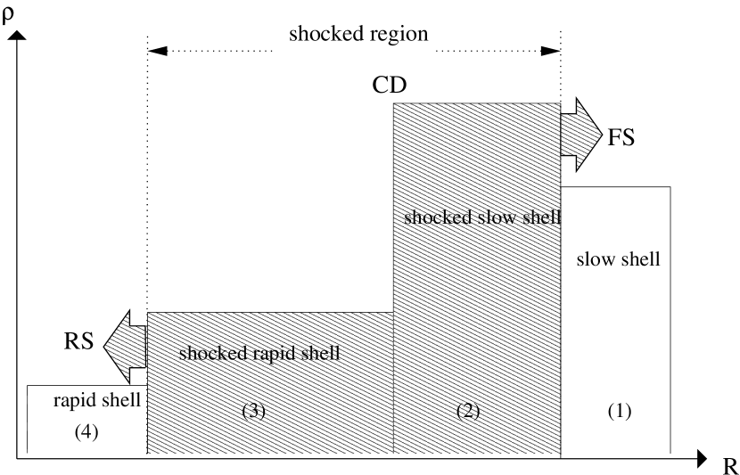
Figure 1: Sketch of a two-shell-collision where a rapid shell catches up with a slower one at the CD frame. Forward and reverse shocks (FS and RS) propagate from the contact discontinuity (CD). We employ the conventional numbering for each region in the study of GRB (e.g., Piran 1999).

In Fig. 1 we draw a schematic mass density profile during the shock propagation in the interactions of rapid and slow shells. Two shocks are formed: a reverse shock that goes into the rapid shell and a forward shock that propagates into the slow shell. There are four regions: (1) the unshocked slow shell, (2) the shocked slow shell, (3) the shocked rapid shell, and (4) the unshocked rapid shell. Thermodynamic quantities, shch as rest mass density $\rho$, pressure $P$, and internal energy density $e$ are measured in the fluid rest frames. We use the terminology of regions $i$ ($i$=1, 2, 3, and 4) and position of discontinuity $j$ ($j$=FS, CD, and RS) where FS, CD, and RS stand for the forward shock front, contact discontinuity, and reverse shock front, respectively. The fluid velocity and Lorentz factor in the region $i$ measured in the ISM rest frame are expressed as $v_{i}(=\beta_{i}c)$, and $\Gamma_{i}$, respectively. The relative velocity and Lorentz factor of the fluids in the regions $i$ and $j$ are denoted as $v_{ij}(=-v_{ji}=\beta_{ij}c=-\beta_{ji}c)$ and $\Gamma_{ij}(=\Gamma_{ji})$, respectively. Throughout this work, we use the assumption of $\Gamma_{i}\gg 1$.

We first count the numbers of quantities and the shock jump conditions. Each region is specified by three physical quantities; rest-mass density $\rho_{i}$, pressure $P_{i}$, and velocity $v_{i}$ measured in the ISM rest frame. Forward and reverse shock speeds measured in the frame of unshocked regions (i.e., regions 1 and 4, respectively) are two other quantities. In all, there are $3\times 4+2=14$ physical quantities. The total number of the jump conditions at the forward shock (FS), reverse shock (RS), and contact discontinuity (CD) is $3+3+2=8$. Hence, given $3+3=6$ upstream quantities for each shock, we can obtain the remaining $8$ downstream quantities by using $8$ jump conditions.

Following Blandford & McKee (1976), we consider the limit of strong shock, $P_{2}/n_{2}\gg P_{1}/n_{1}$, and adopt the assumption that the upstream matter is cold. As an equation of state (EOS), we take

$$P_{i}=(\hat{\gamma}_{i}-1)(e_{i}-\rho_{i})$$ (1)

where $\hat{\gamma}_{i}$ is an adiabatic index. The jump conditions for the forward shock are written as follows:

$$\Gamma_{\rm FS1}^{2}=\frac{(\Gamma_{\rm 12}+1)[\hat{\gamma}_{2}(\Gamma_{\rm 12}-1)+1]^{2}}{\hat{\gamma}_{2}(2-\hat{\gamma}_{2})(\Gamma_{\rm 12}-1)+2},$$

$$e_{2}=\Gamma_{\rm 12}\rho_{2}\,,\qquad\frac{\rho_{2}}{\rho_{1}}=\frac{\hat{\gamma}_{2}\Gamma_{12}+1}{\hat{\gamma}_{2}-1}\,,$$ (2)

where $\Gamma_{12}=\Gamma_{1}\Gamma_{2}(1-\beta_{1}\beta_{2})$, and $\Gamma_{\rm FS1}$ is the Lorentz factor of forward shock measured in the rest frame of the unshocked slow shell. In the relativistic limit, the adiabatic index is ${\hat{\gamma}}_{2}=4/3$. Using the same assumptions as in the forward shock, the jump conditions for the reverse shock are given by:

$$\Gamma_{\rm RS4}^{2}=\frac{(\Gamma_{\rm 34}+1)[\hat{\gamma}_{3}(\Gamma_{\rm 34}-1)+1]^{2}}{\hat{\gamma}_{3}(2-\hat{\gamma}_{3})(\Gamma_{\rm 34}-1)+2},$$

$$e_{3}=\Gamma_{\rm 34}\rho_{3}\,,\qquad\frac{\rho_{3}}{\rho_{4}}=\frac{\hat{\gamma}_{3}\Gamma_{34}+1}{\hat{\gamma}_{3}-1}\,,$$ (3)

where $\Gamma_{34}=\Gamma_{3}\Gamma_{4}(1-\beta_{3}\beta_{4})$, and $\Gamma_{\rm RS4}$ is the Lorentz factor of the reverse shock measured in the rest frame of the unshocked rapid shell. The equality of pressures and velocities across the contact discontinuity gives

$$P_{2}=P_{3},\qquad\Gamma_{2}=\Gamma_{3}\,.$$ (4)

Before a shock breakout, $\Gamma_{2}=\Gamma_{3}=\Gamma_{\rm CD}$ is satisfied. It may be useful to introduce the ratio $f\equiv\rho_{4}/\rho_{1}$, which can be obtained from $P_{2}=P_{3}$, as

$$f\equiv\frac{\rho_{4}}{\rho_{1}}=\frac{(\hat{\gamma}_{2}\Gamma_{12}+1)(\Gamma_{12}-1)}{(\hat{\gamma}_{3}\Gamma_{34}+1)(\Gamma_{34}-1)}\ .$$ (5)

Throughout this paper, we set $P_{1}=P_{4}=0$. Then, we take $\rho_{1}$, $\rho_{4}$, $\Gamma_{1}$, and $\Gamma_{4}$ as ramaining $4$ upstream parameters. Then, with $8$ shock conditions given above, we can obtain $8$ downstream quantities $\rho_{2}$ $e_{2}$, $v_{2}$, $v_{\rm FS}$, $\rho_{3}$, $e_{3}$, $v_{3}$, and $v_{\rm RS}$.

2.2 Time Scales of Wave Propagations

Here we evaluate seven time scales of relevance when the shock and rarefaction waves cross the colliding shells. They are useful to understand the hydrodynamical evolution of two-shell-collisions. We measure these time scales in the rest frame of CD (hereafter we call it the CD frame) because it facilitates the comparison with each other. In contrast, most of the previous papers used the ISM frame in measuring crossing time of shock (e.g., Sari & Piran 1995; Panaitescu et al. 1997). Here we need to introduce new physical paramaters, the shell widths measured in the ISM frame, $\Delta_{\rm r}$, and $\Delta_{\rm s}$, where subscripts $r$ and $s$ represent rapid and slow shells, respectively. In the ISM frame, the upstream parameters are as follows: Lorentz factors $\Gamma_{\rm r}(=\Gamma_{4})$, and $\Gamma_{\rm s}(=\Gamma_{1})$, rest mass densities $\rho_{\rm r}$, and $\rho_{\rm s}$. With $2+4=6$ physical parameters, we can uniquely specify the initial condition. Note that the regions 1 and 4 disappear after FS and RS break out, respectively.

In the CD frame, we rewrite them as follows; $\Delta_{\rm r}^{{}^{\prime}}$, $\Delta_{\rm s}^{{}^{\prime}}$, $\Gamma_{\rm r}^{{}^{\prime}}(=\Gamma_{4}^{{}^{\prime}}=\Gamma_{34})$, and $\Gamma_{\rm s}^{{}^{\prime}}(=\Gamma_{1}^{{}^{\prime}}=\Gamma_{12})$ during the shock propagation in the shells. After the shock breaks out of the shell, the velocity is not uniform and determined by the propagation of rarefaction wave. Note that once we choose the CD frame, $\Gamma_{4}^{{}^{\prime}}$ and $\Gamma_{1}^{{}^{\prime}}$ are not independent of each other (see e.g., Eq. (8) below).

The time in which FS crosses the slow shell, $t_{\rm FS}^{{}^{\prime}}$, is given by

$$t_{\rm FS}^{{}^{\prime}} = \frac{\Delta_{\rm s}^{{}^{\prime}}}{|\beta_{1}^{{}^{\prime}}|+|\beta_{\rm FS}^{{}^{\prime}}|}$$ (6)

$$= \Delta_{\rm s}^{{}^{\prime}}\left[|\beta_{1}^{{}^{\prime}}|+\left(1-\frac{1}{\Gamma_{1}^{{}^{\prime}2}\Gamma_{\rm FS1}^{2}(1-|\beta_{1}^{{}^{\prime}}||\beta_{\rm FS1}|)^{2}}\right)^{1/2}\right]^{-1},$$

where we use Eq. (2.1) and $\beta_{\rm FS}^{{}^{\prime}2}=1-1/\Gamma_{\rm FS}^{{}^{\prime}2}$. Thus, we can express $t_{\rm FS}^{{}^{\prime}}$ as a function of model parameters and $\Gamma_{1}^{{}^{\prime}}$ which is also given implicitly from the model parameters. Similarly, the RS crossing-time in the rapid shell, $t_{\rm RS}^{{}^{\prime}}$, is

$$t_{\rm RS}^{{}^{\prime}} = \frac{\Delta_{\rm r}^{{}^{\prime}}}{|\beta_{4}^{{}^{\prime}}|+|\beta_{\rm RS}^{{}^{\prime}}|}$$ (7)

$$= \Delta_{\rm r}^{{}^{\prime}}\left[|\beta_{4}^{{}^{\prime}}|+\left(1-\frac{1}{\Gamma_{4}^{{}^{\prime}2}\Gamma_{\rm RS4}^{2}(1-|\beta_{4}^{{}^{\prime}}||\beta_{\rm RS4}|)^{2}}\right)^{1/2}\right]^{-1},$$

where we use Eq. (2.1) and $\beta_{\rm RS}^{{}^{\prime}2}=1-1/\Gamma_{\rm RS}^{{}^{\prime}2}$. It is important to note that $\Gamma_{1}^{{}^{\prime}}$ and $\Gamma_{4}^{{}^{\prime}}$ are not independent but related by the equation below,

$$\Gamma_{4}^{{}^{\prime}}=\frac{-f(1-\hat{\gamma}_{3})+\sqrt{f^{2}(1-\hat{\gamma}_{3})^{2}+4f\hat{\gamma}_{3}\left[(\Gamma_{1}^{{}^{\prime}}-1)(\hat{\gamma}_{2}\Gamma_{1}^{{}^{\prime}}+1)+f\right]}}{2f\hat{\gamma}_{3}}.$$ (8)

It is expected that after FS has crossed the slow shell, a rarefaction wave (hereafter we call it FR) propagates into the shocked slow shell (e.g., Panaitescu et al. 1997). The sound speed is given by (e.g., Mihalas & Mihalas 1984)

$$c_{\rm s}^{2}=\left(\frac{\partial P}{\partial e}\right)_{\rm ad}=\frac{\hat{\gamma}P}{e+P}.$$ (9)

Thus, the time at which FR reaches CD, $t_{\rm FR-CD}^{{}^{\prime}}$, is given by

$$t_{\rm FR-CD}^{{}^{\prime}} = t_{\rm FS}^{{}^{\prime}}+\frac{\Delta_{\rm s,FS}^{{}^{\prime}}}{c_{\rm s2}}$$ (10)

$$= t_{\rm FS}^{{}^{\prime}}+\Delta_{\rm s}^{{}^{\prime}}\Gamma_{1}^{{}^{\prime}}\frac{\hat{\gamma}_{2}-1}{\hat{\gamma}_{2}\Gamma_{1}^{{}^{\prime}}+1}\left[\frac{\hat{\gamma}_{2}(\hat{\gamma}_{2}-1)(\Gamma_{1}^{{}^{\prime}}-1)}{\hat{\gamma}_{2}\Gamma_{1}^{{}^{\prime}}-\hat{\gamma}_{2}+1}c^{2}\right]^{-1/2}\ ,$$

where $\Delta_{\rm s,FS}^{{}^{\prime}}$ is the width of the slow shell just after FS reaches the end of the shell. This is obtained by the mass conservation (e.g., Spada et al. 2001) where $(\hat{\gamma}_{2}-1)/(\hat{\gamma}_{2}\Gamma_{1}^{{}^{\prime}}+1)$ is the compression factor of the slow shell and $\Gamma_{1}^{{}^{\prime}}$ is the factor from the Lorentz contraction. Just the same way, the corresponding time, $t_{\rm RR-CD}^{{}^{\prime}}$, at which the rarefaction wave (hereafter we call it RR) generated at the RS breakout reaches CD is given by

$$t_{\rm RR-CD}^{{}^{\prime}} = t_{\rm RS}^{{}^{\prime}}+\frac{\Delta_{\rm r,RS}^{{}^{\prime}}}{c_{\rm s3}}$$ (11)

$$= t_{\rm RS}^{{}^{\prime}}+\Delta_{\rm r}^{{}^{\prime}}\Gamma_{4}^{{}^{\prime}}\frac{\hat{\gamma}_{3}-1}{\hat{\gamma}_{3}\Gamma_{4}^{{}^{\prime}}+1}\left[\frac{\hat{\gamma}_{3}(\hat{\gamma}_{3}-1)(\Gamma_{4}^{{}^{\prime}}-1)}{\hat{\gamma}_{3}\Gamma_{4}^{{}^{\prime}}-\hat{\gamma}_{3}+1}c^{2}\right]^{-1/2}.$$

In the case of $t_{\rm RR-CD}^{{}^{\prime}}>t_{\rm FR-CD}^{{}^{\prime}}$, only $t_{\rm FR-CD}^{{}^{\prime}}$ is an actual time and $t_{\rm RR-CD}^{{}^{\prime}}$ is a virtual time which does not exist in reality. The opposite case is also true.

In the case of $t_{\rm RR-CD}^{{}^{\prime}}<t_{\rm FR-CD}^{{}^{\prime}}$, we have the time at which two rarefaction waves collide each other, $t_{\rm RR-FR}^{{}^{\prime}}$, as

$$t_{\rm RR-FR}^{{}^{\prime}} \sim t_{\rm RR-CD}^{{}^{\prime}}+\frac{\Delta_{\rm s,RR-CD}^{{}^{\prime}}}{2c_{\rm s2}}$$ (12)

$$\sim t_{\rm RR-CD}^{{}^{\prime}}+\frac{\Delta_{\rm s}^{{}^{\prime}}\Gamma_{1}^{{}^{\prime}}}{2c_{\rm s2}}\frac{\hat{\gamma}_{2}-1}{\hat{\gamma}_{2}\Gamma_{1}^{{}^{\prime}}+1}\left(\frac{t_{\rm FR-CD}^{{}^{\prime}}-t_{\rm RR-CD}^{{}^{\prime}}}{t_{\rm FR-CD}^{{}^{\prime}}-t_{\rm FS}^{{}^{\prime}}}\right),$$

where $\Delta_{\rm s,RR-CD}^{{}^{\prime}}$ is the width of the part of slow shell which FR has not passed through yet at $t_{\rm RR-CD}^{{}^{\prime}}$. Since both RR and FR propagate at the speed $c_{\rm s2}$ after $t_{\rm RR-CD}^{{}^{\prime}}$, the above equation includes factor 2. Note that after the rarefaction wave crosses CD, the pressure gradient appears at CD. As a result, the CD begins to move from $x^{{}^{\prime}}=0$ in the CD frame. Thus, Eqs. (12), (13), (14), and (15) are apploximated estimations. Similarly, in the case of $t_{\rm FR-CD}^{{}^{\prime}}<t_{\rm RR-CD}^{{}^{\prime}}$, we have

$$t_{\rm RR-FR}^{{}^{\prime}} \sim t_{\rm FR-CD}^{{}^{\prime}}+\frac{\Delta_{\rm r,FR-CD}^{{}^{\prime}}}{2c_{\rm s3}}$$ (13)

$$\sim t_{\rm FR-CD}^{{}^{\prime}}+\frac{\Delta_{\rm r}^{{}^{\prime}}\Gamma_{4}^{{}^{\prime}}}{2c_{\rm s3}}\frac{\hat{\gamma}_{3}-1}{\hat{\gamma}_{3}\Gamma_{4}^{{}^{\prime}}+1}\left(\frac{t_{\rm RR-CD}^{{}^{\prime}}-t_{\rm FR-CD}^{{}^{\prime}}}{t_{\rm RR-CD}^{{}^{\prime}}-t_{\rm RS}^{{}^{\prime}}}\right).$$

The time scale in which RR catches up with the propagating forward shock (FS), $t_{\rm RR-FS}^{{}^{\prime}}$, can be estimated as

$$t_{\rm RR-FS}^{{}^{\prime}}\sim\frac{c_{\rm s,2}t_{\rm RR-CD}^{{}^{\prime}}}{c_{\rm s2}-\beta_{\rm FS}^{{}^{\prime}}c}\ .$$ (14)

Similarly, the time-scale in which FR catches up with the reverse shock (RS) is approximated as

$$t_{\rm FR-RS}^{{}^{\prime}}\sim\frac{c_{\rm r,3}t_{\rm FR-CD}^{{}^{\prime}}}{c_{\rm s3}-\beta_{\rm RS}^{{}^{\prime}}c}\ .$$ (15)

2.3 Numerical Simulation

We complementarily perform the special relativistic hydrodynamical simulations. The detail of the code is given in Mizuta et al. (2004). To sum up, the code is based on an approximate relativistic Riemann solver. The numerical flux is derived from Marquina’s flux formula (Donat & Marquina 1996). This code is originally second order in space using the so-called MUSCL method. In this study, however, this is slightly compromised for numerical stability. We assume plane symmetry and treat one dimensional motions of shells. In discussing the propagation of shock and rarefaction waves, we choose the CD frame. Given the ratio $\Gamma_{\rm r}/\Gamma_{\rm s}$ in the ISM frame and the value of $\Gamma_{\rm s}$, we can determine the Lorentz transformation to the CD frame easily because the CD Lorentz factor $\Gamma_{\rm CD}(=\Gamma_{2}=\Gamma_{3})$ measured in the ISM frame can be derived by solving Eq. (5). We should note that the number of free parameters is reduced from 6 to 5 because we have already fixed the frame. As for the EOS, we assume for simplicity that $\hat{\gamma}_{3}=\hat{\gamma}_{2}=4/3$ for $\Gamma_{34}>2$, and $\hat{\gamma}_{3}=\hat{\gamma}_{2}=5/3$ otherwise. Although this simplification gives slightly inaccurate estimation on the speeds of wave propagations, there is little effect on our conclusions in this work.

We start the calculation at $t=0$ when the collision of two shells has just begun. Thoughout this paper, we set $\Delta_{s}^{{}^{\prime}}/c=1$ and $\rho_{r}=1$ as units in numerical simulations. Initially, two shells have opposite velocities, namely, $v_{\rm r}^{{}^{\prime}}>0$ and $v_{\rm s}^{{}^{\prime}}<0$. In the previous section, we did not impose any conditions for the plasma surrounding the two shells. We only assumed that the boundary of each shell will be kept intact during the passage of shocks and rarefaction waves. For our numerical runs, we put plasma of low rest mass density $(10^{-4}\ll 1,\rho_{\rm s}/\rho_{\rm r})$ outside of the two shells. They have the same velocity and pressure as the adjacent shell. At first, the boundary condition at the left boundary is a steady inflow of dilute plasma. When the reverse shock or the rarefaction wave reaches the rapid shell’s boundary, the velocity of the dilute plasma is set to be zero instantaneously to reduce the effect of the interaction between the shock and the dilute plasma. At the same time, the left boundary condition is set to be a free outflow. The treatment of the right side dilute plasma and the boundary condition is the same as that of the left side.

3 SHELL DYNAMICS AFTER COLLISION

3.1 Shell Splitting

3.1.1 General Consideration

Here we classify the types of the mass density profile in the merged shell based on the order of the times obtained in the previous section. Table 1 gives the complete set of the possible orders. Although there are various cases in the orders, the density profile, in particular, the splitting feature is governed by the two criteria as follows.

1. When $t_{\rm RR-CD}^{{}^{\prime}}<t_{\rm FR-CD}^{{}^{\prime}}$ for $\rho_{\rm r}>\rho_{\rm s}$ or $t_{\rm FR-CD}^{{}^{\prime}}<t_{\rm RR-CD}^{{}^{\prime}}$ for $\rho_{\rm s}>\rho_{\rm r}$ is satisfied, the splitting occurs at the CD since the rarefaction wave going from the larger density region (region 2) into the smaller density region (region 3) makes a dip in the latter region.

2. When a pair of rarefaction waves propagating in the opposite directions collide with each other, the density begins to decrease at the collision point and the splitting feature emerges. Hence the existence of $t_{\rm RR-FR}$ implies splitting feature.

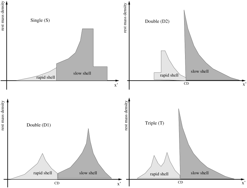
Figure 2: Schematic snapshot of the rest mass density of two shells. Here we assume $\rho_{\rm s}>\rho_{\rm r}$. The corresponding time scale relation in each case is shown in Table 1. Picture S shows the case where RR catches up with the propagating FS and has a single-peak. Picture D1 shows the case where both of FS and RS cross the shells and the rarefaction waves propagating from both sides dig a dip and give a double-peaked profile. Picture D2 shows the case where FR reaches CD and dig a dip. Hence the profile is double-peaked. Picture T shows the case of the combination of D1 and D2. Then the final profile is triple-peaked.

Based on these two criteria, the mass density profile is classified into four types and shown in Fig. 2. If both criteria are satisfied, then the mass density has triple peaks. We show the corresponding schematic picture of space time diagram in Fig. 3. If only one criteria is met, then the double-peaked profile is realized. When neither condition is satisfied, the single peak is obtained.

3.1.2 GRBs and Blazars

Here we apply the above general consideration to the specific cases and examine which kind of rest mass density profile is realized in GRBs and blazars. We assume that the widths of two shells are same in the ISM frame which is written as $\Delta_{\rm r}/\Delta_{\rm s}=1$ (see, e.g., KS01). We consider following three cases since it seeems natural to suppose that ejected shells from the central engine have a correlation among them; (1) the energy of bulk motion of the rapid shell ($E=\Gamma mc^{2}$) equals to that of the slow one in the ISM frame (we refer to it as “equal energy (or $E$)”), (2) the mass of rapid shell ($m=\rho\Gamma\Delta$) equals to that of the slow one (hereafter we call it “equal mass (or $m$)”), and (3) the rest mass density of rapid shell equals to that of the slow one (hereafter we call it “equal rest mass density (or $\rho$)”),

$$\rho_{\rm r} = \rho_{\rm s}\qquad({\rm equal}\ \rho),$$

$$\rho_{\rm r}\Delta_{\rm r}\Gamma_{\rm r} = \rho_{\rm s}\Delta_{\rm s}\Gamma_{\rm s}\qquad({\rm equal}\ m),$$

$$\rho_{\rm r}\Delta_{\rm r}\Gamma_{\rm r}^{2}c^{2} = \rho_{\rm s}\Delta_{\rm s}\Gamma_{\rm s}^{2}c^{2}\qquad({\rm equal}\ E).$$ (16)

Note that in the case of $\Delta_{\rm r}=\Delta_{\rm s}$ and $\Gamma_{\rm r}>\Gamma_{\rm s}$, $\rho_{\rm s}$ is always larger than $\rho_{\rm r}$. This leads to the absence of $t_{\rm RR-FS}$. For all cases, we have $3+1+1=5$ parameters. We take the ratio $\Gamma_{\rm r}/\Gamma_{\rm s}$ as the last parameter and vary its value. This completes the six model parameters.

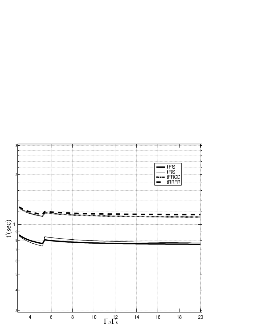
Figure 4: $\Gamma_{\rm r}/\Gamma_{\rm s}$ dependence of the various time scales for the “equal E”case. In the whole range, case 4 (Triple) is realized. The slight jumps of the time scales at $\Gamma_{\rm r}/\Gamma_{\rm s}\sim 5$ correspond to the abrupt change of adiabatic index. The softening of EOS in the relativistic regime gives slower shock waves and the time scales get longer accordingly.

The various time scales for the “equal $E$” case in GRBs are shown as a function of $\Gamma_{\rm r}/\Gamma_{\rm s}$ in Fig. 4. Here we set $\Gamma_{\rm s}=10^{2}$, $\Delta_{\rm s}^{{}^{\prime}}=10^{10}$ cm, and $\rho_{\rm s}=10^{-10}$ g cm^-3 in the slow shell as an example. Slight jumps of time scales are seen at $\Gamma_{\rm r}/\Gamma_{\rm s}\sim 5$ in the Figure. They are caused by the abrupt change of adiabatic index between the non-relativistic regime and relativistic one. The softening of EOS in the relativistic regime leads to slower shock waves propagation in the CD frame. In the whole range, the criteria (I) and (II) given in the previous section are both satisfied. Therefore, the triple-peaked profile is expected (No. 4 in Table 1) in principle. However, the criterion (I) is satisfied only marginally. As a result, two peaks are not remarkable. It is worthwhile to obtain order estimations of $\Delta_{\rm r}^{{}^{\prime}}/\Delta_{\rm s}^{{}^{\prime}}$ and $|\beta_{\rm r}^{{}^{\prime}}/\beta_{\rm s}^{{}^{\prime}}|$ by using a simple apploximation of $\Gamma_{\rm CD}\sim\Gamma_{\rm m}$ ($\Gamma_{\rm m}$ is the Lorentz factor of marged shell obtained by two-mass-collision model and it is given in the next subsection) in spite of some discrepancy with the exact solution of Eq. (5). We have

$$\frac{\Delta_{\rm r}^{{}^{\prime}}}{\Delta_{\rm s}^{{}^{\prime}}}=\frac{\Delta_{\rm r}\Gamma_{\rm r}\Gamma_{\rm s}^{{}^{\prime}}}{\Delta_{\rm s}\Gamma_{\rm s}\Gamma_{\rm r}^{{}^{\prime}}}\simeq\left(\frac{\Gamma_{4}}{\Gamma_{1}}\right)^{2}\left(\frac{\Gamma_{1}^{2}+\Gamma_{2}^{2}}{\Gamma_{3}^{2}+\Gamma_{4}^{2}}\right),\qquad\left|\frac{\beta_{\rm r}^{{}^{\prime}}}{\beta_{\rm s}^{{}^{\prime}}}\right|\simeq\frac{(\Gamma_{1}^{2}+\Gamma_{2}^{2})(-\Gamma_{3}^{2}+\Gamma_{4}^{2})}{(-\Gamma_{1}^{2}+\Gamma_{2}^{2})(\Gamma_{3}^{2}+\Gamma_{4}^{2})}.$$ (17)

As $\Gamma_{\rm r}/\Gamma_{\rm s}$ increases, the ratios of shell widths and velocities in the CD frame go asymptotically to

$$\frac{\Delta_{\rm r}^{{}^{\prime}}}{\Delta_{\rm s}^{{}^{\prime}}}\sim 3,\qquad\left|\frac{\beta_{\rm r}^{{}^{\prime}}}{\beta_{\rm s}^{{}^{\prime}}}\right|\sim 3.$$ (18)

This equation explains well the fact that each time scale in Fig. 4 has a weak dependence on $\Gamma_{r}/\Gamma_{s}$. This is the reason why $t_{\rm RS}^{{}^{\prime}}$ and $t_{\rm FS}^{{}^{\prime}}$ are very close to each other. $t_{\rm RR-CD}^{{}^{\prime}}$ is also close to $t_{\rm FR-CD}^{{}^{\prime}}$ simply because the sound speeds in the both shocked regions are about a few ten percents of the light speed and close to each other. The corresponding numerical results are shown in Figs. 5 and 6. In these calculations, we take the cases of $\Gamma_{\rm r}/\Gamma_{\rm s}=3$ and $\Gamma_{\rm r}/\Gamma_{\rm s}=6$, respectively. This implies a large density contrast of $\rho_{\rm s}/\rho_{\rm r}=9$ and $\rho_{\rm s}/\rho_{\rm r}=36$, respectively (see Table 2). The collision of the rarefaction waves occurs in the region with much lower density compared with region 2. As a result, the peak of the profile is smoothed out. For larger values of $\Gamma_{\rm r}/\Gamma_{\rm s}$, the density contrast between regions 2 and 3 becomes clearer. Hence we conclude that the “equal energy” case essencially evolves into single-peaked profiles. The space-time diagram obtained by the numerical simulation for “equal $E$” is shown in Figs. 5 and 6. From Fig. 5, we see that $t_{\rm FS}^{{}^{\prime}}\sim t_{\rm RS}^{{}^{\prime}}\sim 3$ as is shown in Eq. (18). In Fig. 6, these time scales become close to $3$.

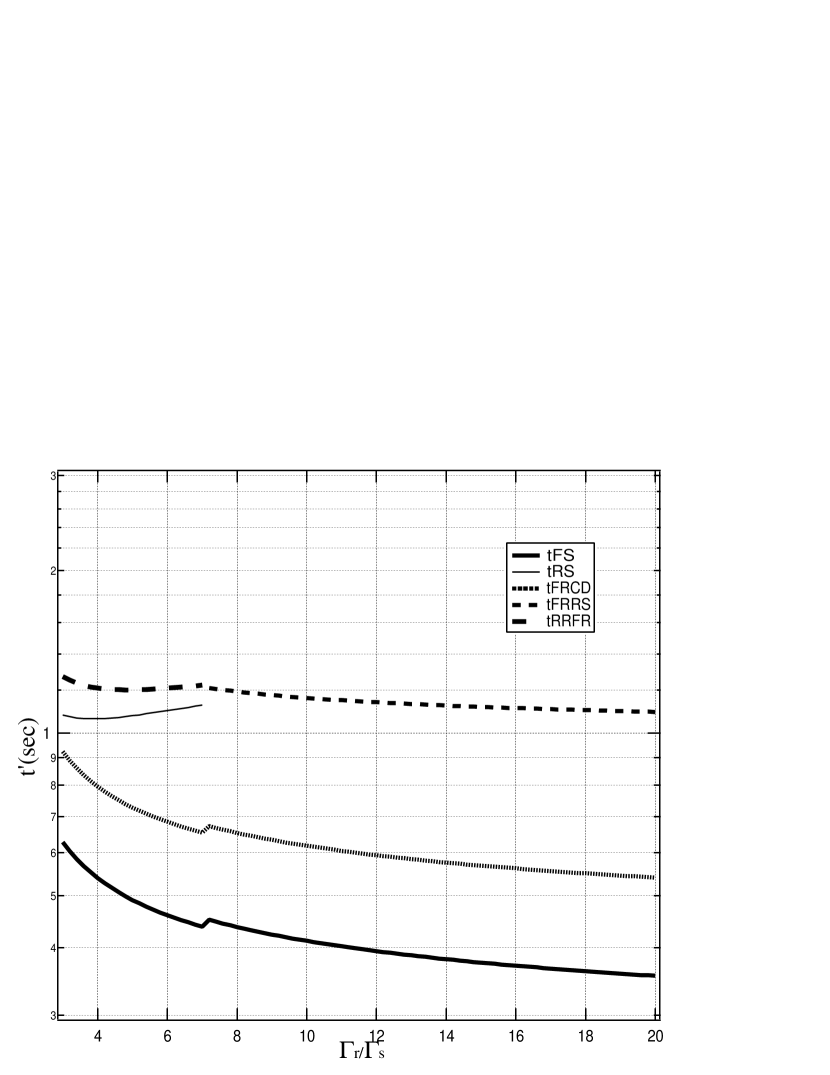
Figure 7: Time scales for “equal mass”. When $\Gamma_{\rm r}/\Gamma_{\rm s}$ is smaller than $\sim 7$, case 6 (Triple) is realized. For $\Gamma_{\rm r}/\Gamma_{\rm s}$ larger than $\sim 7$, case 5 (D2) is realized. The slight jumps of the time scales at $\Gamma_{\rm r}/\Gamma_{\rm s}\sim 7$ correspond to the abrupt change of adiabatic index. The softening of EOS in the relativistic regime gives slower shock waves and the time scales get longer accordingly.

The time scales for the “equal mass” case are shown in Fig. 7. Up to $\Gamma_{\rm r}/\Gamma_{\rm s}\sim 20$, the criteria (I) and (II) are both satisfied and the triple-peaked profile shows up (No. 6 in Table 1). As $\Gamma_{\rm r}/\Gamma_{\rm s}$ increases, we obtain

$$\frac{\Delta_{\rm r}^{{}^{\prime}}}{\Delta_{\rm s}^{{}^{\prime}}}\sim\frac{\Gamma_{4}}{\Gamma_{1}},\qquad\left|\frac{\beta_{\rm r}^{{}^{\prime}}}{\beta_{\rm s}^{{}^{\prime}}}\right|\sim 1,$$ (19)

and $t_{\rm RS}^{{}^{\prime}}$ and $t_{\rm RR-CD}^{{}^{\prime}}$ become larger compared with $t_{\rm FS}^{{}^{\prime}}$ and $t_{\rm FR-CD}^{{}^{\prime}}$. For the numerical experiment, we select two cases which have $\Gamma_{\rm r}/\Gamma_{\rm s}=3$ and $20$. In each case, we clearly see the dip corresponding to the criterion (I) in Figs. 8 and 9. However, as in the “equal $E$” case, the collision of rarefaction waves occurs in the less dense rapid shell and the density peak tends to be smoothed out. Hence we conclude that the equal mass collision with a large value of $\Gamma_{\rm r}/\Gamma_{\rm s}$ effectively evolves in to the double-peaked (D2) profile. In KS01, the authors found a shell-split feature in their numerical simulation (Fig. 2 in their paper) for the “equal $m$” case. It can be also explained as the D2 profile. In Fig. 9, we see that the rarefaction wave (FR) driven by the breakout of FS catches up with the shock wave (RS) from behind at $t^{{}^{\prime}}\sim 3$, since the flow seen from RS is subsonic in the downstream of RS. The propagation speed of RS is modified by the merge with the rarefaction wave and is determined by the strengths of the shock wave and rarefaction wave. For the current case, the propagation speed of RS is almost unchanged up to its breakout at $t^{{}^{\prime}}\lesssim 5.4$.

The time scales for the “equal $\rho$” case is shown in Fig. 11. The important point is that $\rho_{\rm s}=\rho_{\rm r}$ along CD. Then the criterion (I) disappears. In the limit of large $\Gamma_{\rm r}/\Gamma_{\rm s}$, we have

$$\frac{\Delta_{\rm r}^{{}^{\prime}}}{\Delta_{\rm s}^{{}^{\prime}}}\sim\frac{1}{3}\left(\frac{\Gamma_{4}}{\Gamma_{1}}\right)^{2}\qquad\left|\frac{\beta_{\rm r}^{{}^{\prime}}}{\beta_{\rm s}^{{}^{\prime}}}\right|\sim\frac{1}{3},$$ (20)

and $t_{\rm RS}$ and $t_{\rm RR-CD}$ become larger compared with $t_{\rm FS}$ and $t_{\rm FR-CD}$. We see this in the numerical experiment with $\Gamma_{\rm r}/\Gamma_{\rm s}=6$ in Fig. 11. As in Fig. 9, we see also in Fig. 11 that the FR catches up to the RS and merges during $3\lesssim t^{{}^{\prime}}\lesssim 6.5$. The last topic is the dependence of the above results on the hitherto fixed model parameters $\Gamma_{\rm s}$, $\Delta_{\rm s}^{{}^{\prime}}$, and $\rho_{\rm s}$. The results for different $\Gamma_{\rm s}$ are completely the same as in Fig. 4. The position of each time scale is determined by $\Delta_{\rm r}^{{}^{\prime}}/\Delta_{\rm s}^{{}^{\prime}}$ and $\beta_{\rm r}^{{}^{\prime}}/\beta_{\rm s}^{{}^{\prime}}$ and they are independent of $\Delta_{\rm s}$ itself. Hence we omit corresponding figures. For different $\rho_{\rm s}$, the result is also almost unchanged, since we treat the case of $\Gamma_{\rm r}/\Gamma_{\rm s}>3$ for simplicity. Then the sound speed is about a few ten percent of the light speed and has a weak dependence on $\rho_{\rm s}$. When $\Delta_{\rm s}^{{}^{\prime}}$ is increased, every time-scale increases linearly keeping the relative positions of the time scales.

For a typical blazar, we set up three slow shell parameters as $\Gamma_{\rm s}=10$, $\Delta_{\rm s}^{{}^{\prime}}=10^{16}$ cm, and $\rho_{\rm s}=10^{-26}\rm\ g\ cm^{-3}$. We show the result in Fig. 12 for the “equal $E$” case as an example. The essential difference between GRBs and blazars is a typical shell width. Hence, as explained above, every time-scale becomes $10^{6}$ times larger than that in Fig. 4 with the relative positions unchanged.

3.1.3 Extra case

Since we have not seen so far a clear case corresponding to the criterion (II), we have performed another specific case to show what happens for the collision of two rarefaction-rarefaction waves collision (D1 profile in Fig. 2). D1 profile is appears most clearly when the rapid and slow shells have similar mass densities and shell widths in the CD frame. Hence we do not use the assumption of $\Delta_{\rm r}=\Delta_{\rm s}$ here only. Instead, we employ the condition that $\rho_{\rm r}=\rho_{\rm s}$, $\Delta^{{}^{\prime}}_{\rm r}=\Delta^{{}^{\prime}}_{\rm s}$, and $\Gamma_{\rm r}/\Gamma_{\rm s}=20$. In Fig. 13, D1 profile is indeed produced. A larger value of $\Gamma_{\rm r}/\Gamma_{\rm s}$ produce a greater dip than that shown in Fig. 13.

3.2 Shell Spreading

In principle, we can obtain the speed of rarefaction wave using Riemann invariants (e.g., Zel’dovich & Raizer, 1966). In the relativistic limit, it is known that the speed of the head of rarefaction wave is close to the speed of light (e.g., Anile 1989). As the EOS of the shocked region deviates from the relativistic one, the speed is reduced from the light speed and the intermediate regime should be treated by numerical calculations (e.g., Wen, Panaitescu, & Laguna 1997). It is worthwhile to note that from the values $\Gamma_{\rm r}^{{}^{\prime}}$ and $\Gamma_{\rm s}^{{}^{\prime}}$ in Table 2 we see that the EOS in the forward-shocked region is a non-relativistic one while the reverse-shocked region extends from the non-relativistic to the relativistic regime for the parameter ranges we adopted.

Numerical results for shell spreading are shown in Figs. 5, 6, 8, 9, and 11, in which the width of the shell may be described as

$$\Delta_{\rm tot}^{{}^{\prime}}(t^{{}^{\prime}})\simeq\Delta_{\rm s,FS}^{{}^{\prime}}+\Delta_{\rm r,RS}^{{}^{\prime}}+v_{\rm FE}(t^{{}^{\prime}}-t_{\rm FS}^{{}^{\prime}})+v_{\rm RE}(t^{{}^{\prime}}-t_{\rm RS}^{{}^{\prime}}),$$ (21)

where $\Delta_{\rm tot}^{{}^{\prime}}$ is the total width of the shell in the CD frame. We should stress that although a lot of authors assume that the shell width is not changed after collisions (e.g., Spada et al. 2000; NP02) for simplicity, the reality is that the shells spread at $v_{\rm FE}$ and $v_{\rm RE}$ in the forward and backward directions, respectively.

3.3 Energy Conversion Efficiency

The conversion efficiency of the bulk kinetic energy to the internal one is one of the most important issues to explore the nature of the central engine of relativistic outflows and many authors have studied it (e.g., Kumar 1999; Tanihata et al. 2002).

3.3.1 Two-mass-collision model

Let us briefly review the widely-used two-mass-collision model (e.g., Piran 1999). From the momentum and energy conservations, we have

$$m_{\rm r}\Gamma_{\rm r}+m_{\rm s}\Gamma_{\rm s} = (m_{\rm m}+{\cal E}_{\rm m}/c^{2})\Gamma_{\rm m},$$

$$m_{\rm r}\Gamma_{\rm r}\beta_{\rm r}+m_{\rm s}\Gamma_{\rm s}\beta_{\rm s} = (m_{\rm m}+{\cal E}_{\rm m}/c^{2})\Gamma_{\rm m}\beta_{\rm m},$$ (22)

where $m_{\rm m}=m_{\rm r}+m_{\rm s}$, ${\cal E}_{\rm m}={\cal E}_{\rm r}+{\cal E}_{\rm s}$, and $\Gamma_{\rm m}$ are the mass, the internal energy, and the Lorentz factor of the merged shell, respectively, and $m_{\rm r}$ and $m_{\rm s}$ are the rest mass of the rapid and slow shells, respectively. Then we obtain the efficiency $\epsilon$ as

$$\epsilon=1-\frac{(m_{\rm r}+m_{\rm s})\Gamma_{\rm m}}{m_{\rm r}\Gamma_{\rm r}+m_{\rm s}\Gamma_{\rm s}},\qquad\Gamma_{\rm m}^{2}=\Gamma_{\rm r}\Gamma_{\rm s}\frac{m_{\rm r}\Gamma_{\rm r}+m_{\rm s}\Gamma_{\rm s}}{m_{\rm r}\Gamma_{\rm s}+m_{\rm s}\Gamma_{\rm r}}.$$ (23)

It is a useful shortcut to approximate $\Gamma_{\rm m}\sim\Gamma_{2}=\Gamma_{3}$ without solving Eq. (5). Using this shortcut, for the “equal mass density” case ($m_{\rm r}/\Gamma_{\rm r}=m_{\rm s}/\Gamma_{\rm s}$), we have $\Gamma_{\rm m}^{2}=(\Gamma_{\rm r}^{2}+\Gamma_{\rm s}^{2})/2$. For the “equal mass” case ($m_{\rm r}=m_{\rm s}$), we have $\Gamma_{\rm m}^{2}=\Gamma_{\rm r}\Gamma_{\rm s}$. For “equal energy” ($m_{\rm r}\Gamma_{\rm r}=m_{\rm s}\Gamma_{\rm s}$), we have $\Gamma_{\rm m}^{2}=2(\Gamma_{\rm s}^{2}\Gamma_{\rm r}^{2})/(\Gamma_{\rm s}^{2}+\Gamma_{\rm r}^{2})$. Then, the efficiency $\epsilon$ in each case is given by

$$\epsilon \simeq \left\{\begin{array}[]{ll}1-\frac{1}{\sqrt{2}}\left(1+\frac{\Gamma_{\rm s}}{\Gamma_{\rm r}}\right)\left[1+\left(\frac{\Gamma_{\rm s}}{\Gamma_{\rm r}}\right)^{2}\right]^{-1/2}&({\rm equal}\ \rho),\\ 1-\left(\frac{4}{2+\frac{\Gamma_{\rm r}}{\Gamma_{\rm s}}+\frac{\Gamma_{\rm s}}{\Gamma_{\rm r}}}\right)^{1/2}&({\rm equal}\ m),\\ 1-\frac{1}{\sqrt{2}}\left(1+\frac{\Gamma_{\rm r}}{\Gamma_{\rm s}}\right)\left[1+\left(\frac{\Gamma_{\rm r}}{\Gamma_{\rm s}}\right)^{2}\right]^{-1/2}&({\rm equal}\ E).\\ \end{array}\right.$$ (27)

As the value of $\Gamma_{r}/\Gamma_{s}$ gets larger for the “equal $m$” case, the efficiency becomes larger and approaches $\sim 1$. For “equal $E$” and “equal $\rho$” cases, it goes asymptotically to $\sim 0.3$. Thus we find that “equal $m$” is the most effective collision if we neglect the rarefaction waves.

3.3.2 Shock model

The consideration of shock dynamics provides us with the information of the assignment of the total dissipation energy $E_{\rm diss}$ to the forward- and reverse-shocked regions $E_{\rm FS}$ and $E_{\rm RS}$. From the equations of mass continuity in the CD frame, we have $\frac{\Delta_{\rm s,FS}^{{}^{\prime}}}{\Delta_{\rm s}^{{}^{\prime}}}=\frac{\Gamma_{1}^{{}^{\prime}}(\hat{\gamma}_{2}-1)}{\hat{\gamma}_{2}\Gamma_{1}^{{}^{\prime}}+1}$ and $\frac{\Delta_{\rm s,RS}^{{}^{\prime}}}{\Delta_{\rm r}^{{}^{\prime}}}=\frac{\Gamma_{4}^{{}^{\prime}}(\hat{\gamma}_{3}-1)}{\hat{\gamma}_{3}\Gamma_{4}^{{}^{\prime}}+1}$ Assuming a large value of $\Gamma_{4}/\Gamma_{1}$, then we have $e_{2}+P_{2}\simeq e_{3}+P_{3}$ and the dissipated energies are mainly controlled by shell widths. They are written as

$$\frac{E_{\rm FS}}{E_{\rm diss}}\simeq\frac{\Delta_{\rm s,FS}^{{}^{\prime}}}{\Delta_{\rm s,FS}^{{}^{\prime}}+\Delta_{\rm r,RS}^{{}^{\prime}}},\quad\frac{E_{\rm RS}}{E_{\rm diss}}\simeq\frac{\Delta_{\rm r,RS}^{{}^{\prime}}}{\Delta_{\rm s,FS}^{{}^{\prime}}+\Delta_{\rm r,RS}^{{}^{\prime}}}$$ (28)

where $E_{\rm FS}$ and $E_{\rm RS}$, internal energy of forward and reverse shocked regions just after the shock crosses each shell, respectively (e.g., Spada et al. 2000). However, the values $E_{\rm FS}/E_{\rm diss}$ and $E_{\rm RS}/E_{\rm diss}$ will begin to deviate from the the above approximation when the rarefaction waves start to propagate, since they reconvert the internal energy into the kinetic one. The result including the rarefaction waves is shown below.

3.3.3 Numerical Results

The estimation of the energy conversion efficiencies with shock and rarefaction waves taken into account are presented in Figs. 14, 15 and 16 based on the numerical simulations. From the analogy of the two-mass-collision model, we define the efficiency measured in the ISM frame as

$$\epsilon(t) \equiv 1-\frac{\int\Gamma(t,x)~{}dm(t,x)}{\Gamma_{\rm r}m_{\rm r}+\Gamma_{\rm s}m_{\rm s}}$$ (29)

$$= 1-\frac{\int\Gamma(t,x)~{}\rho(t,x)\Gamma(t,x)dx}{\rho_{\rm r}\Delta_{r}\Gamma_{\rm r}^{2}+\rho_{\rm s}\Delta_{s}\Gamma_{\rm s}^{2}},$$

where $dm(t,x)$, $\rho(t,x)$, $\Gamma(t,x)$, and $\Gamma(t,x)dx$, are the rest mass element, the rest mass density, and the Lorentz factor, seen in the ISM frame, and the length of line element in the CD frame, respectively. We assume the origins of both frames coinside with each other at $t=t^{{}^{\prime}}=0$. The Lorentz transformation of $\Gamma(t,x)$ is wtitten as $\Gamma(t,x)=\Gamma_{\rm CD}\Gamma^{{}^{\prime}}(t,x)[1-\beta_{\rm CD}\beta^{{}^{\prime}}(t,x)]$. The hypersurface of a constant time in the ISM frame does not coinside with that in CD frame. Hence, to evaluate spatial integrations at a certain time in the ISM frame, we must collect the values of physical quantities in the inegrand for different times in the CD frame. Unfortunately it is technically difficult task to perform this. Hence we report to an approximation that $\rho(t,x)$ and $\Gamma(t,x)$ are replaced by $\rho(t^{{}^{\prime}},x^{{}^{\prime}})$ and $\Gamma(t^{{}^{\prime}},x^{{}^{\prime}})$, respectively. This is only valid near the original point of the CD frame and, elsewhere, mixes up those quantities at the different time slice. We believe, however, that this still gives the behavior of the efficiency and the essencial role of rarefaction waves. In these figures, we compare the numerical results with the prediction by the two-mass-collision approximation. We find that the two-mass-collision model well reproduces the hydrodynamical results just before rarefaction waves begin to propagate. After the shock waves break-out the shells, the conversion effeciency is reduced by several ten percent from the estimate of the two-mass-collision model after several dynamical times. It is noted again that no cooling effect is taken into account here.

4 SUMMARY AND DISCUSSION

In this paper we have illuminated the difference between the simple two-mass-collision model and the hydrodynamical one of the internal shock. We have studied 1D hydrodynamical simulations of the two-shell-collisions in the CD frame taking the shock and rarefaction waves into account. Below we summarize our results and give some discussions.

(1) By comparing the relevant time scales of shock and rarefaction waves, we have completely classified the evolutions of the two-shell-collisions using six physical parameters, that is, the widths, rest mass densities, and velocities of the two colliding shells. We find that rarefaction waves have a significant effect on the dynamics. In principle, the rest mass density profile can be evolved into single-, double-, and triple-peaked features. In the limit of $\Gamma_{\rm r},\Gamma_{\rm s}\gg 1$, the features are essentially characterized by only three parameters: the ratios of Lorentz factors, widths, and rest mass densities. The combination of the values of $\Gamma_{\rm r}/\Gamma_{\rm s}$ and $\rho_{\rm r}/\rho_{\rm s}$ determines the relative orders of the time scales of various wave propagations, while the value of $\Delta_{\rm r}/\Delta_{\rm s}$ controls normarizations of the time scales.

(2) Bearing in mind the application to relativistic outflows such as GRBs and blazars, we specifically examine the cases of “equal $\rho$”, “equal $m$”, and “equal $E$”. For the “equal $\rho$” case, the profile is single-peaked. The rarefaction wave produced when the FS breaks out reaches CD and then catches up with RS. In the case of “equal $m$”, the profile should in principle become triple-peaked according to our classification scheme. In practice, however, there is very little time for the FR-RR collision to make a clear dip, while there is a lot more time for the FR to create a dip for a fairly wide range of parameters. Therefore, the profile in this case is effectively double-peaked. For the “equal $E$” case, the profile is classified as triple-peak. However, again, there is very little time for the FR-RR collision to make a dip. A very large mass-density gradient between forward- and reverse-shocked regions makes the dip even less pronounced. Furthermore, there is again little time for FR to create a dip for a fairly wide range of parameters. Hence, we conclude that the profile for the “equal $E$” is effectively single-peakd. If the cooling time scale is sufficiently long in the shocked region, electromagnetic radiations will show these profiles.

(3) For large $\Gamma_{\rm r}/\Gamma_{\rm s}$, we have shown that the spreading velocity of the shells after collision is close to the speed of light. Hence, the often used approximation of constant shell width after collision is not very good in treating multiple collisions. For examle, the authors in NP02 claim that the “equal energy” case is suggested for the shell Lorentz factors in GRBs, assuming that $L>\Delta$, where $L$ is the separation distance between two shells. If the interval of the first and the second collisions is long, however, the shell spreading effect cannot be ignored and the case of $L<\Delta$ should be included in the analysis. Then the difference between the “equal $m$” and “equal $E$” cases might be wiped away.

(4) As the shell spreads after collision, the internal energy is converted back to the bulk kinetic energy due to thermal expansion. We have numerically studied the time-dependent energy conversion efficiency quantitatively. Since we have neglected cooling processes, the conversion effciency rises up to the order of unity. This should be corresponding to the event in the regime of “weak cooling” (Kino & Takahara 2004). If $\Gamma_{\rm r}/\Gamma_{\rm s}\gg 1$ and the time-interval between collisions is long, the conversion efficiency will be substantially deviated the estimate of the two-mass-collision model.

We appreciate the insightful comments and suggestions of the referee. M.K. thank S. Kobayashi, K. Asano and F. Takahara for useful remarks and discussions. A.M. acknowledges support from Japan Sosiety for the Promotion of Science (JSPS). This work is also supported in part by the Grant-in-Aid Program for Scientific Research (14340066, 14740166 and 14079202) from the Ministry of Education, Science, Sports, and Culture of Japan.

Table 1: Various types of the evolution

No.	$\rho$	timescalea	profileb
1	$\rho_{\rm s}>\rho_{\rm r}$	$t_{\rm RS}^{{}^{\prime}}<t_{\rm RR-CD}^{{}^{\prime}}<t_{\rm RR-FS}^{{}^{\prime}}$	S
2		$t_{\rm RS}^{{}^{\prime}}<t_{\rm RR-CD}^{{}^{\prime}}<t_{\rm FS}^{{}^{\prime}}<t_{\rm RR-FR}^{{}^{\prime}}$	D1
3		$t_{\rm RS}^{{}^{\prime}}<t_{\rm FS}^{{}^{\prime}}<t_{\rm RR-CD}^{{}^{\prime}}<t_{\rm RR-FR}^{{}^{\prime}}$	D1
4		$t_{\rm RS}^{{}^{\prime}}<t_{\rm FS}^{{}^{\prime}}<t_{\rm FR-CD}^{{}^{\prime}}<t_{\rm RR-FR}^{{}^{\prime}}$	T
5		$t_{\rm FS}^{{}^{\prime}}<t_{\rm FR-CD}^{{}^{\prime}}<t_{\rm FR-RS}^{{}^{\prime}}$	D2
6		$t_{\rm FS}^{{}^{\prime}}<t_{\rm FR-CD}^{{}^{\prime}}<t_{\rm RS}^{{}^{\prime}}<t_{\rm RR-FR}^{{}^{\prime}}$	T
7		$t_{\rm FS}^{{}^{\prime}}<t_{\rm RS}^{{}^{\prime}}<_{\rm FR-CD}^{{}^{\prime}}<t_{\rm RR-FR}^{{}^{\prime}}$	T
8		$t_{\rm FS}^{{}^{\prime}}<t_{\rm RS}^{{}^{\prime}}<_{\rm RR-CD}^{{}^{\prime}}<t_{\rm RR-FR}^{{}^{\prime}}$	D1
9	$\rho_{\rm s}<\rho_{\rm r}$	$t_{\rm RS}^{{}^{\prime}}<t_{\rm RR-CD}^{{}^{\prime}}<t_{\rm RR-FS}^{{}^{\prime}}$	D2
10		$t_{\rm RS}^{{}^{\prime}}<t_{\rm RR-CD}^{{}^{\prime}}<t_{\rm FS}^{{}^{\prime}}<t_{\rm RR-FR}^{{}^{\prime}}$	T
11		$t_{\rm RS}^{{}^{\prime}}<t_{\rm FS}^{{}^{\prime}}<t_{\rm RR-CD}^{{}^{\prime}}<t_{\rm RR-FR}^{{}^{\prime}}$	T
12		$t_{\rm RS}^{{}^{\prime}}<t_{\rm FS}^{{}^{\prime}}<t_{\rm FR-CD}^{{}^{\prime}}<t_{\rm RR-FR}^{{}^{\prime}}$	D1
13		$t_{\rm FS}^{{}^{\prime}}<t_{\rm FR-CD}^{{}^{\prime}}<t_{\rm FR-RS}^{{}^{\prime}}$	S
14		$t_{\rm FS}^{{}^{\prime}}<t_{\rm FR-CD}^{{}^{\prime}}<t_{\rm RS}^{{}^{\prime}}<t_{\rm RR-FR}^{{}^{\prime}}$	D1
15		$t_{\rm FS}^{{}^{\prime}}<t_{\rm RS}^{{}^{\prime}}<t_{\rm FR-CD}^{{}^{\prime}}<t_{\rm RR-FR}^{{}^{\prime}}$	D1
16		$t_{\rm FS}^{{}^{\prime}}<t_{\rm RS}^{{}^{\prime}}<t_{\rm RR-CD}^{{}^{\prime}}<t_{\rm RR-FR}^{{}^{\prime}}$	T
17	$\rho_{\rm s}=\rho_{\rm r}$	$t_{\rm RS}^{{}^{\prime}}<t_{\rm RR-FS}^{{}^{\prime}}$	S
18		$t_{\rm RS}^{{}^{\prime}}<t_{\rm FS}^{{}^{\prime}}<t_{\rm RR-FR}^{{}^{\prime}}$	D1
19		$t_{\rm FS}^{{}^{\prime}}<t_{\rm FR-RS}^{{}^{\prime}}$	S
20		$t_{\rm FS}^{{}^{\prime}}<t_{\rm RS}^{{}^{\prime}}<t_{\rm RR-FR}^{{}^{\prime}}$	D1

Table 2: Parameter sets for numerical simulations of “equal $E$”, “equal $m$” and “equal $\rho$”.

No.a	$\Gamma_{\rm r}/\Gamma_{s}$	$\Gamma_{\rm CD}$b	$\Gamma_{\rm r}^{{}^{\prime}}$	$\Gamma_{\rm s}^{{}^{\prime}}$	$\Delta_{\rm r}^{{}^{\prime}}/\Delta_{\rm s}^{{}^{\prime}}$	$\rho_{\rm s}/\rho_{\rm r}$
4(equal $E$)	3	6.7	1.34	1.05	2.3	9
4(equal $E$)c	6	7.0	2.26	1.06	2.8	36
6(equal $m$)	3	7.6	1.25	1.09	2.6	3
5(equal $m$)c	20	11.8	4.29	1.40	6.4	20
19(equal $\rho$)	6	12.2	1.43	1.43	6.0	1
–(equal $\rho$)c d	20	22.4	2.35	2.35	1.0	1

Figure 3: Schematic picture of space-time diagram of a two-shell-interaction in the CD frame. Here we assume $\rho_{\rm s}>\rho_{\rm r}$. A forward shock (FS) and a reverse shock (RS) run through the slow and rapid shells, respectively. After the shocks break out, the rarefaction waves propagate into the shells (FR and RR) and the shells spread (FE and RE). This corresponds to case 7 in Table 1.

Figure 5: Left: Time evolution of the rest mass density profile in the CD frame in the case of “equal $E$”. The parameter is chosen so that $\Gamma_{\rm r}/\Gamma_{\rm s}=3$ in the ISM frame. The parameters in the CD frame are shown in Table 2. Throughout our numerical simulations, we set $\Delta_{\rm s}^{{}^{\prime}}/c=1$ and $\rho_{\rm s}=1$ as units. Right: Space-time diagram of shock and rarefaction waves propagations. As is shown in the text, $t_{\rm RS}\sim t_{\rm FS}\sim 3$. RE spreads at the speed $\sim 0.9c$ while FE spreads at the speed $\sim 0.6c$.

Figure 6: Left: Time evolution of the rest mass density profile in the CD frame for “equal $E$”. In the ISM frame, $\Gamma_{\rm r}/\Gamma_{\rm s}=6$. The parameters are given in Table 2. Right: Space-time diagram of shock and rarefaction waves propagations. Both FS and RS propagate faster than those for $\Gamma_{\rm r}/\Gamma_{\rm s}=3$ and $t_{\rm FS}\sim t_{\rm RS}\sim 3$. RE spreads at the speed $\sim c$ while FE spreads at the speed $\sim 0.7c$.

Figure 8: Left: Time evolution of the rest mass density profile in the CD frame for “equal $m$”. In the ISM frame $\Gamma_{\rm r}/\Gamma_{\rm s}=3$. The parameters are shown in Table 2. Criterion (II) is satisfied and the profile classified “D2” in Fig. 2 is seen in this numerical result. Space-time diagram of shock and rarefaction waves propagations. RE spreads at the speed $\sim 0.8c$ while FE spreads at the speed $\sim 0.7c$.

Figure 9: Left: Time evolution of the rest mass density profile in the CD frame for “equal $m$”. In the ISM frame, $\Gamma_{\rm r}/\Gamma_{\rm s}=20$. The parameters are shown in Table 2. The dilute rapid shell collides with the slow one and quickly spreads out. We also see that the dense slow shock is pushed forwards by the rapid shell. Right: Space-time diagram of shock and rarefaction waves propagations. RE spreads at the speed $\sim c$ while FE spreads at the speed $\sim 0.9c$.

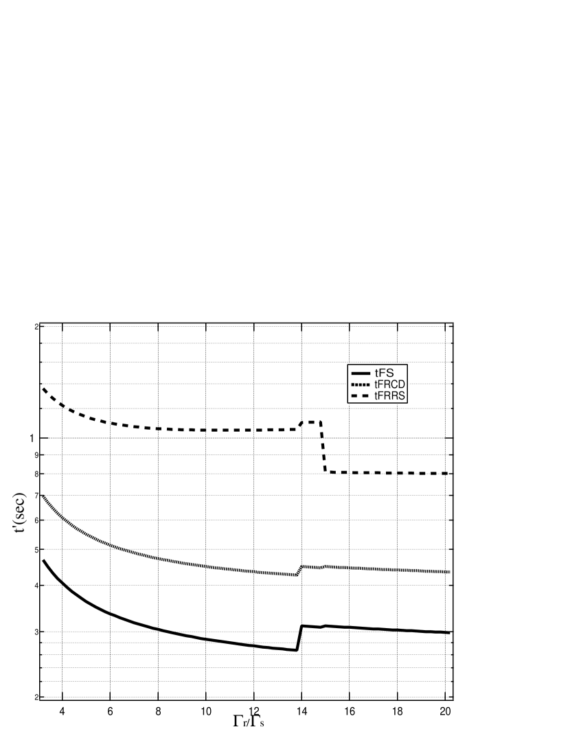
Figure 10: Time scales for “equal $\rho$”. Case 19 in Table 1 is realized in the whole range. The slight jumps of the time scales at $\Gamma_{\rm r}/\Gamma_{\rm s}\sim 14,15$ correspond to the abrupt change of adiabatic index. The softening of EOS in the relativistic regime gives slower shock waves and the time scales get longer accordingly.

Figure 11: Left: Time evolution of the rest mass density profile in the CD frame for “equal $\rho$”. In the ISM frame, $\Gamma_{\rm r}/\Gamma_{\rm s}=6$. The parameters are shown in Table 2. Right: Space-time diagram of shock and rarefaction waves propagations. RE spreads at the speed $\sim c$ while FE spreads at the speed $\sim 0.8c$.

Figure 12: The same as Fig. 4 but for blazars. Compared with Fig. 4 the relative positions of various time scales are almost unchanged while the absolute value of each time-scale is reduced by a factor of $10^{6}$ which is the ratio of the shell width of GRB to that of blazar.

Figure 13: Left: Time evolution of the rest mass density profile in the CD frame for “equal $\rho$”. In the ISM frame, $\Gamma_{\rm r}/\Gamma_{\rm s}=20$. The parameters are shown in Table 2. By the rarefaction-rarefaction wave collision, the bump is generated at the center of the shell. This corresponds to the D1 profile in Fig. 2. Right: Space-time diagram of shock and rarefaction waves propagations. Both RE and FE spread at the speed $\sim c$.

Figure 14: Left: Time evolutions of the conversion efficiency defined by Eq. (29) for the “equal energy” case. During shock propagations, $\epsilon$ approaches the two-mass-collision estimate given by Eq. (27) for each case. As the rarefaction waves begin to propagate, the efficiencies are reduced by them. This suppression is can be ascribed to the thermal expansion.

Figure 15: Time evolutions of the conversion efficiency defined by Eq. (29) for the “equal $m$” case. During shock propagations, $\epsilon$ approaches the two-point-mass estimate given by Eq. (27) for each case.

Figure 16: Time evolutions of the conversion efficiency defined by Eq. (29) for the “equal $\rho$” case. During shock propagations, $\epsilon$ approaches the two-point-mass estimate given by Eq. (27) for each case.

References

- (1) Anile, A. M. 1989, Relativistic Fluids and Magnetofluids, Cambridge Univ. Press, Cambridge
- (2) Blandford, R. D. & McKee, C. F. 1976, Physics of Fluids, 19, 1130
- (3) Donat, R. & Marquina, A. 1996, J. Comp. Phys., 125, 42
- Fishman & Meegan (1995) Fishman, G. J. & Meegan, C. A. 1995, ARA&A, 33, 415
- (5) Harrison, F. A. et al. 2001, ApJ, 559, 123
- Kaiser, Sunyaev, & Spruit (2000) Kaiser, C. R., Sunyaev, R., & Spruit, H. C. 2000, A&A, 356, 975
- (7) Kino M., Takahara F., Kusunose M., 2002, ApJ, 564, 97
- (8) Kino M., & Takahara F., 2004, MNRAS, 349, 336
- Kobayashi, Piran, & Sari (1997) Kobayashi, S., Piran, T., & Sari, R. 1997, ApJ, 490, 92
- Kobayashi & Sari (2001) Kobayashi S., Sari R., 2001, ApJ, 551, 934 (KS01)
- Komissarov & Falle (1997) Komissarov, S. S. & Falle, S. A. E. G. 1997, MNRAS, 288, 833
- Kumar (1999) Kumar, P. 1999, ApJ, 523, L113
- (13) Landau, L. D., & Lifshitz, E. M. 1959, Fluid Mechanics, Pergamon Press, Oxford
- (14) Mihalas, D., & Mihalas, B.W. 1984, Foundations of Radiation Hydrodynamics, Oxford Univ. Press, Oxford
- Mizuta, Yamada, & Takabe (2004) Mizuta, A., Yamada, S., & Takabe, H. 2004, ApJ, in press
- Nakar & Piran (2002) Nakar, E. & Piran, T. 2002, ApJ, 572, L139 (NP02)
- Panaitescu et al. (1997) Panaitescu A., Wen L., Laguna P., Meszaros P., 1997, ApJ, 482, 942
- Piran (1999) Piran, T. 1999, Phys. Rep, 314, 575
- (19) Rees, M. J. 1978, MNRAS, 184, 61
- Rees & Meszaros (1994) Rees, M. J. & Meszaros, P. 1994, ApJ, 430, L93
- Sari & Piran (1995) Sari, R. & Piran, T. 1995, ApJ, 455, L143
- (22) Spada, M., Ghisellini, G., Lazzati, D., & Celotti, A. 2001, MNRAS, 325, 1559
- Takahashi et al. (2000) Takahashi, T. et al. 2000, ApJ, 542, L105
- (24) Tanihata, C., Takahashi, T., Kataoka, J., & Madejski, G. 2003, ApJ, in 584, 153
- Wen, Panaitescu, & Laguna (1997) Wen, L., Panaitescu, A., & Laguna, P. 1997, ApJ, 486, 919
- Wijers & Galama (1999) Wijers, R. A. M. J. & Galama, T. J. 1999, ApJ, 523, 177
- (27) Ya. B. Zel’dovich, & Yu. P. Raizer, 1966, Physics of Shock Waves and High-Temperature Phenomena, Academic, New York