Sunyaev-Zeldovich effect in WMAP and its effect on cosmological parameters

Abstract

We use multi-frequency information in first year WMAP data to search for the Sunyaev-Zeldovich (SZ) effect. WMAP has sufficiently broad frequency coverage to constrain SZ without the addition of higher frequency data: the SZ power spectrum amplitude is expected to increase 50% from W to Q frequency band. This, in combination with the low noise in WMAP, allows us to strongly constrain the SZ contribution. We derive an optimal frequency combination of WMAP cross-spectra to extract SZ in the presence of noise, CMB, and radio point sources, which are marginalized over. We find that the SZ contribution is less than 2% (95% c.l.) at the first acoustic peak in W band. Under the assumption that the removed radio point sources are not correlated with SZ this limit implies $\sigma_{8}<1.07$ at 95% c.l. We investigate the effect on the cosmological parameters of allowing an SZ component. We run Monte Carlo Markov Chains with and without an SZ component and find that the addition of SZ does not affect any of the cosmological conclusions. We conclude that SZ does not contaminate the WMAP CMB or change cosmological parameters, refuting the recent claims that they may be corrupted.

I Introduction

Wilkinson Microwave Anisotropy Probe Bennett et al. (2003a) (WMAP) observations of the Cosmic Microwave Background (CMB) have ushered in a new era of high precision observational cosmology. Such a tremendous increase in data quality requires a corresponding increase in the care that goes into the data analysis and interpretation. One of the lingering concerns surrounding the analysis is the residual effect from additional sources of anisotropies. A very prominent candidate among these is the Sunyaev-Zeldovich effect (SZ). Electrons in hot gas scatter photons and distort the blackbody spectrum of the CMB. Galaxy clusters, where gas is the hottest, contribute the bulk of the effect, shock-heating the gas in their potential wells. Radio and microwave band observations pointed at known clusters routinely yield SZ detections, so this effect is now well established observationally. The scattering preferentially raises the energy of the CMB photons, but the number of scatterings is low, so the process never achieves thermal equilibrium. Therefore SZ appears as a CMB temperature decrement at low frequencies and as an increment at high frequencies. This frequency dependence is well known: it is constant in the Rayleigh-Jeans (RJ) regime of the blackbody spectrum, and is universal (independent of gas temperature or density) for non-relativistic electrons.

In the channels of WMAP, SZ is a temperature decrement. Table 1 provides WMAP’s frequency bands, and the SZ frequency dependence in those bands. The K and Ka bands are the most heavily polluted by galactic contamination, so the best prospects for identifying SZ in WMAP are in the differencing assemblies of the upper three bands: two assemblies in Q, two in V, and four in W. While it is usually argued that SZ is indistinguishable from the CMB in the WMAP channels this is actually not so: in CMB temperature units the SZ power spectrum increases by 50% from W to Q channel and in W it is only 61% of the RJ power. We will show that this suffices to place strong constraints on SZ using WMAP data alone, a consequence of the remarkably low noise in WMAP data.

Band	$\nu$ (GHz)	${\Delta T^{\text{SZ}}/(T^{\text{CMB}}y)}$	$C_{l}/C_{l}^{\text{RJ}}$
K	23	$-1.97$	$0.972$
Ka	33	$-1.94$	$0.945$
Q	41	$-1.91$	$0.915$
V	61	$-1.81$	$0.820$
W	94	$-1.56$	$0.611$

Table 1: SZ contribution in the bands of WMAP. We note the band name, frequency, temperature perturbation relative to the comptonization parameter $y$, which does not depend on frequency, and power spectrum relative to the power in the Rayleigh-Jeans regime. In the WMAP bands, SZ is a temperature decrement. In the Rayleigh-Jeans regime, ${\Delta T^{\text{SZ}}/(T^{\text{CMB}}y)}=-2$.

In the literature, several groups have attempted to identify SZ in WMAP data using cross-correlations with other tracers of large scale structure (LSS). In Bennett et al. (2003b) they build an SZ template from the XBACs catalog of x-ray clusters Ebeling et al. (1996), and fit for the amplitude of SZ, arguing for a $2.5\sigma$ detection. In Afshordi et al. (2003) they compute the cross-power spectra of the 2MASS extended source catalog Jarrett et al. (2000) with WMAP’s Q, V, and W bands, then fit for the amplitude of the SZ signal, arguing for a 3.1–3.7$\sigma$ detection of SZ, depending on their mask. In Diego et al. (2003) they compute the cross-power spectrum of the ROSAT diffuse x-ray background maps Snowden et al. (1997) and a WMAP (Q-W) difference map, finding no detection. In Fosalba et al. (2003) they compute the cross-correlation function of SDSS DR1 Abazajian et al. (2003) galaxy survey data with the V band and fit for the amplitude of SZ, finding a 2.7$\sigma$ detection. In Hernández-Monteagudo and Rubiño-Martín (2004) they build templates for SZ from several optical and x-ray cluster surveys, then fit for the amplitude of these templates using maps from the W band and Tegmark et al. (2003), finding no detection for optical clusters and 2–5$\sigma$ detections for x-ray clusters.

Finally, in Myers et al. (2004) they compute the mean temperature in concentric rings about APM Maddox et al. (1990) and ACO Abell et al. (1989) groups and clusters, noting a decrement they attribute to SZ. They interpret this decrement to extend to large scales, $\sim 1$ degree, although the covariance of their bins is unclear. Redshift $z<0.2$ clusters dominate their sample. Their most extreme model assumes that extended SZ emission is representative of the temperature and spatial clustering of gas to $z=0.5$. In this model the SZ power is 30% of the first acoustic peak of the CMB.  Thus they conclude the integrity of the WMAP cosmological parameter fits may be compromised.

In this paper we seek to place limits on SZ from WMAP data alone, thus avoiding any uncertainties in connecting the results of WMAP-LSS cross-correlation to those of WMAP auto-correlation. The cross-correlation methods used before require a model for relating SZ temperature perturbations to some proxies for SZ, which are nonlinear structures such as clusters, and this connection can be quite uncertain. Our method is less model dependent. The downside is that WMAP-only methods sacrifice signal to noise because they do not focus on matter concentrations, where SZ should be strongest, so our method is not optimized for obtaining an SZ detection. However, our main goal is to investigate the amount to which the CMB analysis may be compromised by the residual SZ component, for which we need analysis as model independent as possible.

Our principal method, described in section II, constructs a linear combination of the WMAP Q, V, and W band cross-power spectra which maximizes the contribution of SZ, while at the same time minimizing the radio point source and CMB contribution. We use this linear combination to fit for the SZ power spectrum amplitude, using a spectrum shape from halo model calculations Komatsu and Seljak (2002).

In section III we supplement this method by fitting for cosmological parameters from the WMAP temperature power spectrum using the Markov chain Monte Carlo method, allowing for an additional SZ component in the power spectrum with a free amplitude to be determined by the data. The two methods give consistent results, with the latter giving somewhat weaker constraints. Conclusions are presented in section IV.

II Cross-spectra combination for SZ

We begin our discussion with a simple example. In the absence of noise and point sources, the exact SZ power spectrum could be computed from the difference of any two cross-spectra from different bands. Suppose we took the differencing assemblies from the Q, V and W bands, and compute the cross-power spectra. The SZ power is given by, for example, the difference $($Q1V1$)_{l}-($W1W2$)_{l}=0.25\ C_{l}^{\text{SZ,RJ}}$ in this idealize case, where the coefficient is computed from table 1. Other combinations would also yield the SZ spectrum, with a different coefficient. The important things to note is that the coefficient is not very small and the CMB cancels exactly in this combination: any CMB cosmic variation in the Q and V bands is the same as in the W band, and is subtracted out. In the presence of instrument noise, this difference does not give the exact SZ power spectrum, but a noisy estimate for it. Given a power spectrum shape, we may estimate its amplitude by summing together different $l$ bins, each weighted to give the proper normalization and to emphasize bins with high signal to noise. Our SZ estimator works in this fashion, except that in the presence of point sources, QV$-$WW is a biased estimate. However, by including other cross-spectra, we can form a linear combination of the cross-spectra bins to yield an unbiased estimate for the SZ amplitude. In the following we find such a combination, and apply it to WMAP data.

II.1 Estimator and data

In this section, we introduce our estimator and list the data we use. Our estimator, derived in appendix A, is a generalized version of the point source estimator of Hinshaw et al. (2003).

We want to generate an estimate for SZ from the WMAP cross-spectra. We postulate that the data is the sum of the CMB and two contaminants, radio point sources and SZ. We marginalize point sources and estimate SZ in our main case, which we illustrate in detail below. We consider other cases also, but for brevity omit their details, which are similar. We can write the cross-spectra as

$$\langle C^{\mathbf{i}}_{l}\rangle=C^{\mathbf{i},\rm CMB}_{l}+C^{\mathbf{i},\rm src}_{l}+C^{\mathbf{i},\rm SZ}_{l},$$ (1)

showing explicitly the contribution from each part of the signal. Here the multipole bin is denoted by $l$ and the pair of differencing assemblies in the cross-correlation is denoted by $\mathbf{i}={i_{1}i_{2}}=$ W1W2, Q1V1, etc. No auto-power spectra are included, so we need not worry about noise subtraction.

We will marginalize over the CMB spectrum, which we denote by $C_{l}^{\text{CMB}}$. The window functions for each differencing assembly pair are $\bm{w}=\{w^{\mathbf{i}}_{ll^{\prime}}\}$. We boldface $\bm{w}$ because later we will think of it as a matrix. Therefore the contribution to the cross-spectrum from the CMB is

$$C^{\mathbf{i},\rm CMB}_{l}=\sum_{l}w^{\mathbf{i}}_{ll^{\prime}}C^{\text{CMB}}_{l^{\prime}}.$$ (2)

The spectra we use are in temperature units, and have already been beam-deconvolved, so the window functions $w^{\mathbf{i}}_{ll^{\prime}}=\delta_{ll^{\prime}}$ are trivial. However, it is necessary to keep the window functions explicit in the manipulations that follow.

We denote the amplitude of the point source power spectrum by $A$. This amplitude relates to the cross-spectra via the frequency and shape dependence $\mathbf{S}=\{S^{\mathbf{i}}_{l}\}$. Later we will think of $\mathbf{S}$ as a vector. We take radio sources to have a white noise spectrum with power law frequency dependence, given by:

$$C_{l}^{\mathbf{i},\rm src} = S^{\mathbf{i}}_{l}A$$

$$S^{\mathbf{i}}_{l} = \left(\frac{\nu_{i_{1}}}{\nu_{0}}\right)^{\beta}\left(\frac{\nu_{i_{2}}}{\nu_{0}}\right)^{\beta},$$ (3)

where cross-spectrum $\mathbf{i}$ has channels at $\nu_{i_{1}}$ and $\nu_{i_{2}}$. The units of $A$ are temperature squared. Well-resolved point sources have already been masked from the maps before the evaluation of the cross-spectra, so $A$ represents unresolved sources only. Bennett et al. (2003b) found $\beta=-2.0$ and $\nu_{0}=45$ GHz for the resolved sources. Following Hinshaw et al. (2003) we take the same for the unresolved sources.

We describe amplitude of SZ with $B$, the ratio of the SZ power spectrum and the predicted spectrum, assuming they have the same shape. Thus the SZ amplitude is dimensionless, and has a theoretically predicted value $B=1$ for $\sigma_{8}=0.9$ using the halo models of Komatsu and Seljak (2002). In our notation, this amplitude also relates to the power spectra by the frequency dependence and shape for SZ, which we label $\mathbf{Z}=\{Z^{\mathbf{i}}_{l}\}$. The frequency dependence of a temperature perturbation due to SZ is

$$\frac{\Delta T^{\text{SZ}}}{T^{\text{CMB}}}\propto-2f(x),$$ (4)

where the frequency dependence relative to the RJ regime is given by

$$f(x)=2-\frac{x/2}{\tanh(x/2)},$$ (5)

where $x=h\nu/k_{B}T_{\text{CMB}}$. Note $f\rightarrow 1$ in the RJ limit $x\rightarrow 0$. Thus the SZ contribution to the cross-spectrum is:

$$C_{l}^{\mathbf{i},\rm SZ} = Z^{\mathbf{i}}_{l}B$$

$$Z^{\mathbf{i}}_{l} = C_{l}^{\text{SZ,RJ}}f(\nu_{i_{1}})f(\nu_{i_{2}}),$$ (6)

where the spectrum shape $C_{l}^{\text{SZ,RJ}}$ is from the halo model prediction in the RJ regime using $\sigma_{8}=0.9$, as shown in Figure 3. The shape of SZ is roughly $C_{l}^{\text{SZ,RJ}}\propto l^{-1}$, although it becomes slightly steeper for $l$ greater than a few hundred.

We organize the binned cross-spectra $C^{\mathbf{i}}_{l}$ into a data vector $\mathbf{D}=\{C^{\mathbf{i}}_{l}\}$. We use a Gaussian model for the likelihood $\mathcal{L}$ of the power spectrum:

$$-2\log\mathcal{L}\propto\left[\mathbf{D}-\langle\mathbf{D}\rangle\right]^{{\dagger}}\bm{\Sigma}^{-1}\left[\mathbf{D}-\langle\mathbf{D}\rangle\right].$$ (7)

where the covariance $\bm{\Sigma}=\langle(\mathbf{D}-\langle\mathbf{D}\rangle)(\mathbf{D}-\langle\mathbf{D}\rangle)^{{\dagger}}\rangle$ can be written as $\bm{\Sigma}=\{\Sigma^{\mathbf{ii^{\prime}}}_{ll^{\prime}}\}$. We derive $\bar{B}$, an unbiased estimator for $B$, and its covariance $\Sigma^{B}$ in appendix A. The main result is:

$$\bar{B} \equiv (\mathbf{Z}^{{\dagger}}\mathbf{F}\mathbf{Z})^{-1}\mathbf{Z}^{{\dagger}}\mathbf{F}\mathbf{D}$$

$$\Sigma^{B} \equiv (\mathbf{Z}^{{\dagger}}\mathbf{F}\mathbf{Z})^{-1},$$ (8)

where we have defined the auxiliary matrices

$$\mathbf{F} \equiv \mathbf{E}-\mathbf{E}\mathbf{S}\left(\mathbf{S}^{{\dagger}}\mathbf{E}\mathbf{S}\right)^{-1}\mathbf{S}^{{\dagger}}\mathbf{E}$$

$$\mathbf{E} \equiv \bm{\Sigma}^{-1}-\bm{\Sigma}^{-1}\bm{w}\left(\bm{w}^{{\dagger}}\bm{\Sigma}^{-1}\bm{w}\right)^{-1}\bm{w}^{{\dagger}}\bm{\Sigma}^{-1}$$ (9)

In this notation, we consider $\mathbf{D}$, $\mathbf{S}$, and $\mathbf{Z}$ as column vectors with single index $\mathbf{i}l$, and $\bm{w}$ as matrix with indices $\mathbf{i}l$ and $l^{\prime}$. $\bm{\Sigma}$, $\mathbf{E}$, and $\mathbf{F}$ are matrices with indices $\mathbf{i}l$ and $\mathbf{i}^{\prime}l^{\prime}$. This estimator marginalizes CMB and point sources, which is the most conservative treatment, since it assumes we know nothing about these components. A more aggressive treatment would be to estimate all 3 components simultaneously, but we defer this approach to a future analysis. Note that $\bar{B}$ is a linear combination of the cross-spectra $\mathbf{D}$, with weights $(\mathbf{Z}^{{\dagger}}\mathbf{F}\mathbf{Z})^{-1}\mathbf{Z}^{{\dagger}}\mathbf{F}$.

The data we use consist of the 28 cross-power spectra from the eight differencing assemblies in the WMAP Q, V, and W bands. These spectra are provided at the Legacy Archive for Microwave Background Data Analysis [lam, ]. A galactic foreground model Bennett et al. (2003b) has already been subtracted out. WMAP’s temperature power spectrum is a linear combination of these 28 cross-spectra Hinshaw et al. (2003).

We bin the spectra in $l$, accounting for the number of modes at each $l$. The Legacy Archive does not provide the cross-spectrum covariance, which we need for $\bm{\Sigma}$ in equation (II.1), so we estimate the covariance from the data. We assume the covariance is diagonal in $l$, which is a good approximation Hinshaw et al. (2003). Then in a single bin, we use the dispersion of the cross-spectra about WMAP’s combined temperature power spectrum to estimate $\bm{\Sigma}$ for that bin. (For this purpose we must first un-correct the combined spectrum for the point source contribution.) This procedure to obtain the covariance works best if the power spectrum variance does not change much within a bin and if the bin contains enough $l$’s to get a low-noise estimate of the variance. Our bin width of $\Delta l=40$ is fairly narrow, and gives a covariance which is numerically stable in our subsequent calculations. This technique does not account for the cosmic variance of the CMB, but as we note in the derivation in the appendix, our estimator is insensitive to this source of variance. This makes sense because the CMB is completely projected out, as in our QV$-$WW example at the beginning of section II.

As a test of our estimator, we repeat the estimate of Hinshaw et al. (2003) of the power spectrum amplitude of unresolved point sources. In this case we neither marginalize nor estimate SZ, but assume $B=0$ in equation (II.1). We find a point source amplitude of $A=0.016\pm 0.001\ \mu\text{K}^{2}$, which is roughly consistent with their quoted value of $A=0.015\ \mu\text{K}^{2}$. This gives us confidence in our estimator, despite our covariance matrix constructed from the data.

II.2 Results

We show our estimates for SZ on a bin-by-bin basis, before combining different multipole bins to improve statistics. We marginalize over the CMB and the point source amplitude. Our best estimate for the binned SZ power spectrum is shown in Figure 1. Immediately we can see that the data do not tolerate a large SZ contribution.

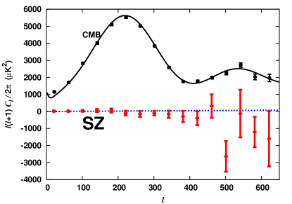
Figure 1: Reconstruction of the SZ power spectrum in the RJ regime, in bins of $\Delta l=40$ (red error bars). There is no visible SZ detection, which would have been positive for this combination. For comparison, we have included the WMAP combined temperature power spectrum, binned the same way, the WMAP best-fit theoretical CMB power spectrum, and a theoretical prediction of SZ in the RJ regime for $\sigma_{8}=0.9$ (blue dotted), calculated from a halo model.

Next we turn to our main case, where we combine all the bins together and estimate the SZ amplitude. Figure 2 shows the weight $(\mathbf{Z}^{{\dagger}}\mathbf{F}\mathbf{Z})^{-1}\mathbf{Z}^{{\dagger}}\mathbf{F}$ for each cross-spectrum in the amplitude estimator. The weights have been divided into groups based on the bands. For plotting, we sum the weights in each group. The bulk of the weight comes from $l=100$ to $l=400$. At lower $l$ there are fewer modes and the SZ contribution is low. At higher $l$ the statistics are limited by detector noise.

The weights are difficult to interpret heuristically. From the frequency dependence, the strength of SZ decreases in order of QQ, QV, VV, QW, VW, and WW. We would expect our combination of cross-spectra would have the SZ-stronger bands minus the SZ-weaker bands. So it is easy to understand the positive weights of QV and QW and the negative weights of VW and WW. Point sources are strongest in Q-band, so a negative weight for QQ makes sense in terms of a point source correction. QW and VW are positive except for bins which are strong in QV. These negative bins may also represent a point source correction

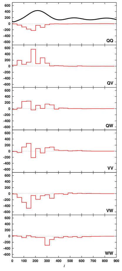
Figure 2: The contribution to the SZ amplitude estimator $\bar{B}$ from the cross-spectra. The horizontal axis is the multipole $l$. The vertical axis show the weight of each spectrum in $\mu$K^-2. We have grouped the cross-spectra by band as noted. Within each group, we have summed the weights of the individual spectra. In the top frame, we have included the CMB power spectrum (arbitrary units) to give scale for $l$.

For the amplitude of SZ relative to the expected RJ amplitude from the halo model with WMAP parameters, our estimator gives us $\bar{B}=-0.042\pm 1.685$. The error is large, and is consistent with both no SZ and the expected $B=1$. Including only the physical region $B>0$, we integrate the likelihood until we include 95% of the probability. From this we quote an upper limit of

$${B}<3.3\quad(95\%).$$ (10)

We plot this limit, along with some models of the SZ power spectrum in Figure 3. At the first acoustic peak, SZ is less than 3% of the CMB in the RJ regime and less than 2% of CMB in W band, on which cosmological parameter estimation is heavily based. We find no evidence for a large SZ contribution. Assuming $C_{l}^{\text{SZ}}\propto(\sigma_{8})^{7}$, this gives a limit of $\sigma_{8}<1.07$ at 95% confidence. To this one should add an additional modeling uncertainty at the level of 10% based on the comparison of predictions from different simulations Komatsu and Seljak (2002). There is a caveat in the upper limit derived here in that we are working with power spectra based on masked maps in WMAP, with more than 200 radio point sources removed. If the SZ signal is correlated with these point sources, which could happen if these radio sources sit in massive clusters Holder (2002), then more SZ may have been removed than expected based on the sky fraction of the mask. This would only affect the $\sigma_{8}$ limits and not the SZ contamination on the primary CMB in the WMAP power spectra. Since we are mostly concerned with the latter we do not explore this issue further. Note that the upper limit on $\sigma_{8}$ is already comparable to the predicted value based on detections from CBI and BIMA, which gives $\sigma_{8}\sim 0.95-1.05$ Readhead et al. (2004); Komatsu and Seljak (2002). It is remarkable that WMAP first year data have sufficient sensitivity to place constraints on the SZ amplitude comparable to other small scale surveys.

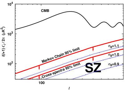
Figure 3: Limit on SZ power spectrum. We present a 95% upper limit on the amplitude of the SZ power spectrum from a combination of WMAP band cross-spectra. We show the temperature fluctuation in the Rayleigh-Jeans regime. For comparison we display the WMAP best fit power spectrum and SZ power spectra from a halo model calculation using $\sigma_{8}=0.9,\,1,\,1.1$.

In the next application we jointly estimate the point source and SZ amplitude, rather than directly marginalizing over the point sources. We find the two parameters to be somewhat correlated (Figure 4), but not to the point of allowing very large SZ amplitude. An extremely strong SZ power is not allowed.

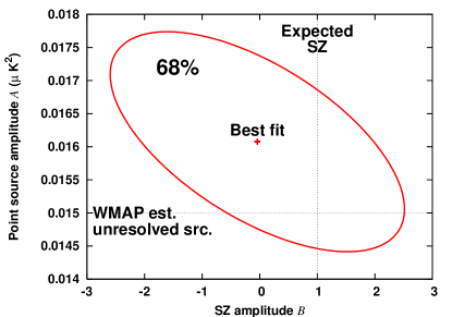
Figure 4: A joint estimation of the SZ power spectrum amplitude and the point source spectrum amplitude. The ellipse encloses 68% of the likelihood. The best fit point is shown by a “$+$”. The vertical line at B=1 shows the theoretically predicted SZ amplitude. The horizontal line shows WMAP’s value for point sources, which does not take into account SZ. Because the power spectrum is a positive quantity, note that portions of the plane where either axis is negative are unphysical.

III Markov chain analysis

In this section we estimate how much SZ signal is in the WMAP $C_{l}$ power spectrum, and investigate the effect of SZ on the determination of the cosmological parameters. For this purpose we use the Markov Chain Monte Carlo (MCMC) approach, using software described in more detail elsewhere Seljak et al. (2003); Slosar et al. (2004).

We ran two MCMCs, one without SZ and one allowing for an unconstrained SZ contribution. We built a third chain from the second by importance sampling, allowing for an SZ component but constraining it to limits derived based on frequency information in the previous section. We used the WMAP likelihood routine Hinshaw et al. (2003); Verde et al. (2003). Each of the chains contains 100,000 total chain elements. The success rate is 45–55 percent, the correlation length is 13–20 elements, and the effective length is 5,000–10,000 elements. Each chain comprises 23 independent sub-chains and, in terms of Gelman and Rubin $\hat{R}$-statistics Gelman and Rubin (1992), we find the chains are sufficiently converged and mixed ($\hat{R}<1.01$, compared to the recommended value of $\hat{R}<1.2$).

In the second chain, we added to the power spectrum an SZ-shaped contribution, parameterized in terms of amplitude $B$ (equation II.1). The WMAP power spectrum combines the Q, V and W bands in different ratios at each $l$, so the shape of the SZ contribution to the WMAP power spectrum is not exactly given by the single frequency SZ template, because the effective frequency for every $l$ varies. This dependence is small and we ignore it here. We find that the SZ contribution to the WMAP combined temperature power spectrum, dominated by V and W channels, may be approximated as 75% the contribution in RJ. One could also add additional CMB experiments (e.g. CBI, VSA, etc.) into the analysis, but this would incur complications to account for the different frequencies of these experiments. In the third chain we add our multi-frequency analysis limit as an additional constraint.

We consider only the simplest model required by the data plus the SZ component, since we want to analyze the effect of the latter on the cosmological parameters. WMAP temperature data require neither tensor modes nor curvature nor running of the primordial power spectrum of the scalar perturbations, so we do not consider them.

We work in a seven parameter space:

$${\mathbf{p}}=\{\omega_{b},\ \omega_{\text{cdm}},\ \Omega_{m},\ \tau,\ A_{s},\ n_{s},\ B\}.$$ (11)

Here $\omega_{b}=\Omega_{b}h^{2}$ is the baryonic content of the universe, $\omega_{\text{cdm}}=\Omega_{\text{cdm}}h^{2}$ is the physical density of the cold dark matter content, $\Omega_{m}=\Omega_{\text{cdm}}+\Omega_{b}=1-\Omega_{\Lambda}$ is the matter density today, $\tau$ is the optical depth to reionization, $A_{s}$ is the amplitude of the primordial scalar perturbations, $n_{s}$ is the primordial slope, and as before $B$ is the amplitude of the SZ power spectrum.

To reduce the degeneracies while running the MCMCs, we use $\omega_{b}$, $\omega_{\text{cdm}}$, angular size of the sound horizon $\Theta_{s}$, $\lg{A_{s}}$, $n_{s}$, $\lg{A_{s}}-\tau-0.5\lg(\omega_{b}+\omega_{\text{cdm}})$, and $B$, instead of the parameters in equation 11. We adopt broad flat priors on these parameters, and additionally require $\tau<0.3$.

We find that the amplitude of an SZ-shaped component to the WMAP power spectrum is limited to $B<7.1$ at 95 percent confidence (see Figure 3). This limit means that the contribution to the WMAP temperature power spectrum at the first peak is below 5 percent. This is a weaker limit than from the combination of cross-spectra, where a factor of 2 better limit was found (equation 10).

	no SZ	with SZ, no SZ prior	with SZ prior
$B$	0	$<7.1$ (95%)	$<2.9$ (95%)
$\omega_{b}\times 10^{2}$	$2.35^{+0.14}_{-0.13}\;{}^{+0.28}_{-0.26}$	$2.51^{+0.21}_{-0.18}\;{}^{+0.47}_{-0.33}$	$2.43^{+0.15}_{-0.15}\;{}^{+0.30}_{-0.29}$
$\Omega_{m}$	$0.245^{+0.07}_{-0.06}\;{}^{+0.15}_{-0.10}$	$0.234^{+0.07}_{-0.06}\;{}^{+0.15}_{-0.10}$	$0.243^{+0.07}_{-0.06}\;{}^{+0.15}_{-0.10}$
$\omega_{\text{cdm}}$	$0.111^{+0.016}_{-0.015}\;{}^{+0.033}_{-0.029}$	$0.111^{+0.016}_{-0.016}\;{}^{+0.033}_{-0.030}$	$0.111^{+0.016}_{-0.016}\;{}^{+0.033}_{-0.031}$
$\tau$	$0.19^{+0.07}_{-0.08}\;{}^{+0.10}_{-0.14}$	$0.20^{+0.07}_{-0.08}\;{}^{+0.10}_{-0.14}$	$0.19^{+0.07}_{-0.08}\;{}^{+0.10}_{-0.14}$
$\sigma_{8}$	$0.88^{+0.12}_{-0.11}\;{}^{+0.25}_{-0.20}$	$0.86^{+0.12}_{-0.11}\;{}^{+0.24}_{-0.22}$	$0.87^{+0.12}_{-0.11}\;{}^{+0.23}_{-0.22}$
$h$	$0.74^{+0.06}_{-0.05}\;{}^{+0.12}_{-0.09}$	$0.76^{+0.07}_{-0.06}\;{}^{+0.14}_{-0.11}$	$0.75^{+0.06}_{-0.05}\;{}^{+0.13}_{-0.10}$
$n_{s}$	$0.99^{+0.04}_{-0.04}\;{}^{+0.07}_{-0.07}$	$0.99^{+0.04}_{-0.04}\;{}^{+0.07}_{-0.07}$	$0.99^{+0.04}_{-0.04}\;{}^{+0.07}_{-0.07}$

Table 2: The first two columns contain the median value and 1- and $2\sigma$ constraints on cosmological parameters for two MCMCs without and with a Sunyaev-Zeldovich component in the $C_{l}$ power spectrum from WMAP data alone. For both chains there was an imposed prior of $\tau<0.3$. The third column shows the constraints when the limit on SZ from our cross-spectrum estimator is applied as a prior.

Table 2 shows the comparison of the two MCMCs, showing the effect of including SZ in the analysis. The inclusion of the additional parameter $B$ into the likelihood analysis affects only the determination of the baryon physical density $\omega_{b}$. Without SZ we find $\omega_{b}=0.0235$, whereas with SZ we find $\omega_{b}=0.0251$, which is shifted by about $1.5\sigma$ away from the earlier value. The confidence contours in the $(\omega_{b},B)$ plane are shown in Figure 5, showing that there is a degeneracy between these two parameters. However, we can and should also use the constraint from our multi-frequency cross-spectrum analysis as a prior. We can include the Gaussian likelihood for $B$ from section II, and perform importance sampling of the chain with SZ. We then find $\omega_{b}=0.0243$, different from the case without SZ by $0.6\sigma$. The likelihood contours including the prior are also shown in Figure 5. The other parameters are much less affected by the SZ.

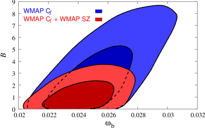
Figure 5: We show two-dimensional contours of 68% and 95% confidence levels in $(\omega_{b},B)$ plane. The larger (blue) contours show the degeneracy using the WMAP combined temperature power spectrum without any prior on SZ. The smaller (red) contours include our multi-frequency cross-spectrum analysis as a prior. $B=1$ is expected from halo models for SZ when $\sigma_{8}=0.9$.

The next largest deviation from the first chain to the second is a shift in the median $h$ of about $0.3\sigma$ towards higher value, which is not statistically significant and the effect is even smaller if the constraints from previous section are added to the chains.

IV Conclusions

We have analyzed the WMAP power spectra in two ways and found them to be free of serious contamination from SZ. The more powerful and less model dependent of the two methods is to use multi-frequency information: by combining the WMAP cross-spectra, we limit at 95% confidence the amplitude of SZ to be below 2% of the CMB at the position of first peak in W band. By searching for an SZ-shaped component in the WMAP combined spectrum with a Markov chain Monte Carlo we also do not find any evidence of a signal, but we can only set a weaker limit. Combining the analyses, we show that the cosmological parameters are not affected by the SZ within the range allowed by the multi-frequency analysis.

There are several possible improvements in the analysis that could further tighten the limits and may be applied to the second year data once they become available. In addition to having lower noise, the two year data are also expected to have better control of systematics such as beam uncertainties and noise correlations.

First, we would like to improve our method for obtaining the cross-spectrum covariance matrix. The estimate for the covariance is noisy, which makes our weights for combining the power spectra noisier than they should be. If we double the size of the bins we average over to obtain the covariance, our limit changes slightly ($B<4.3$ opposed to $B<3.3$ at 95%) and the point source estimate is virtually unchanged. However, it is impossible to tell if this effect is due to a covariance matrix with less noise (which is better) or due to weights whose wide bins combine high- and low-signal-to-noise multipoles less optimally (which is worse). This can be improved if the WMAP second year data release includes the cross-spectrum covariance matrix.

The second possible improvement of our analysis is to improve the frequency dependence of point sources or the WMAP beam deconvolution, both of which can bias our estimate. Our estimator is only unbiased if the models one applies to it are faithful to the data. The models we have used are the best available, and this information will improve in the second year data. It seems unlikely that these improvements will strongly modify the conclusions in this paper.

The third improvement is to perform the analysis on the maps which do not have point sources excised. As discussed above, masking of resolved point sources from the WMAP data may reduce the SZ signal if the two are correlated. This would weaken our limit on $\sigma_{8}$ from the absence of SZ signal, but does not change our conclusions about the effect of SZ on the CMB and cosmological parameters. Still, given that the current limits are reaching the levels of interest it is worth exploring this possibility further.

The fourth improvement is to verify the assumed shape for the SZ power spectrum. This is currently based on halo models, since hydrodynamic simulations cannot simulate sufficiently large volumes to make predictions reliable. If the power spectrum has a radically different shape, our limit is hard to interpret, but the level of contamination on primary CMB is likely to remain unchanged, as is clear from Figure 1. As an example we estimated the SZ in bins of $\Delta l=120$. In the bin containing the first acoustic peak, we limit the SZ power to 4.9 times the halo model power predictions at 95% confidence or 4% contamination in W. It is clear that as long as the SZ spectrum is smooth the limits on the contamination are not going to change significantly over the range with best sensitivity at $100<l<300$.

Finally, our procedure to marginalize over CMB and point sources is conservative and the errors could be further reduced if a joint estimation is used instead. We know something more about the CMB power spectrum than just its frequency dependence, and in this case we can use this information. We also note that a relatively trivial modification to WMAP’s method for estimating the power spectrum could eliminate any contaminant with an SZ-like shape and frequency dependence, much in the same way that they eliminate point sources. However, the fact that we find no residual SZ effects implies that this procedure is not really required and justifies the treatment of the WMAP team in ignoring SZ.

Even with future data detecting the SZ power spectrum from WMAP alone may be difficult. If the bulk of the covariance is from noise, it would take WMAP roughly 3 years to get a 1$\sigma$ detection of SZ using the cross-spectrum combination method of this paper, if $\sigma_{8}=0.9$. Elimination of non-noise sources of covariance, such as uncertainties remaining in the beams, may help. If $\sigma_{8}=1$ then a 2$\sigma$ detection should be possible with 4 year data and one should start seeing a hint of the signal already with 2 year data. Theoretical predictions remain somewhat uncertain, so it is possible that these predictions have a systematic uncertainty of around 10%, but it is clear that it will be worth looking for SZ in future WMAP releases.

Appendix A Cross-spectrum contaminant estimator

In this appendix we present a generalized version of the point source estimator of Hinshaw et al. (2003), using a vector notation. We discuss contaminants in general and do not mention point sources or SZ specifically. We assume we know the power spectrum shape and frequency dependence of all contaminants.

Our data are the cross-power spectra from the experiment. Let vector $\mathbf{D}=\{C^{\mathbf{i}}_{l}\}$ be these spectra. The multipole (or multipole bin) is denoted by $l$ and the cross correlation is denoted by $\mathbf{i}=$ W1W2, W1V1, etc. We use a Gaussian model for the likelihood $\mathcal{L}(\mathbf{D})$ of the set of cross-spectra:

$$-2\log\mathcal{L}\propto\left[\mathbf{D}-\langle\mathbf{D}\rangle\right]^{{\dagger}}\bm{\Sigma}^{-1}\left[\mathbf{D}-\langle\mathbf{D}\rangle\right].$$ (12)

where the covariance $\bm{\Sigma}=\langle(\mathbf{D}-\langle\mathbf{D}\rangle)(\mathbf{D}-\langle\mathbf{D}\rangle)^{{\dagger}}\rangle$ can be written as $\bm{\Sigma}=\{\Sigma^{\mathbf{ii^{\prime}}}_{ll^{\prime}}\}$.

We postulate that the data $\mathbf{D}$ is the sum of the CMB and a number of contaminants. For each of these contributions to the data we need a model, and parameters for that model. Some of these parameters we will estimate, and some we will marginalize.

First we consider the CMB. The parameters which describe the CMB are the band powers: $C_{l}$. We organize these band powers into a vector $\mathbf{C}=\{C_{l}\}$. We will later marginalize over these parameters. To relate the CMB parameters to the data we use the window function $\bm{w}=\{w^{\mathbf{i}}_{ll^{\prime}}\}$ for each cross spectrum channel pair. We may think of the window function as the response of the instrument to a given set of CMB $C_{l}$’s. In the absence of noise and contaminants, the data would be given by the matrix multiplication $\mathbf{D}=\bm{w}\mathbf{C}$.

We use as similar notation for the contaminants. We describe each contaminant by a power spectrum shape, a frequency dependence, and an amplitude. We take the shapes and frequency dependences as given, and the amplitudes as parameters. We divide the amplitude parameters into two groups, those to marginalize and those to estimate. The amplitude parameters to marginalize we denote by vector $\mathbf{A}=\{A_{\alpha}\}$, where $\alpha$ runs over the components to marginalize. The amplitude parameters to estimate we denote by vector $\mathbf{B}=\{B_{\beta}\}$, where $\beta$ runs over the components to estimate.

We may think of the shape and frequency dependences as the response of the instrument to a given set of contaminant amplitudes. Thus the shape dependence already includes the influence of the window function. Similarly to the amplitudes, we divide the shape and frequency dependences into two groups. The shape and frequency dependence of the contaminants to marginalize we write as $\mathbf{S}=\{S^{\mathbf{i}}_{l\alpha}\}$. The shape and frequency dependence of the contaminants to estimate we write as $\mathbf{Z}=\{Z^{\mathbf{i}}_{l\beta}\}$. In the absence of CMB and noise, the data would be given by $\mathbf{D}=\mathbf{S}\mathbf{A}+\mathbf{Z}\mathbf{B}$.

If we include all components and uncorrelated noise, then we can write the expected data as

$$\langle\mathbf{D}\rangle=\bm{w}\mathbf{C}+\mathbf{S}\mathbf{A}+\mathbf{Z}\mathbf{B}.$$ (13)

We are considering cross-spectra only, and have included no noise term.

We substitute into the likelihood expression:

$$-2\log\mathcal{L} \propto \left[\mathbf{D}-(\bm{w}\mathbf{C}+\mathbf{S}\mathbf{A}+\mathbf{Z}\mathbf{B})\right]^{{\dagger}}\bm{\Sigma}^{-1}$$ (14)

$$\qquad\left[\mathbf{D}-(\bm{w}\mathbf{C}+\mathbf{S}\mathbf{A}+\mathbf{Z}\mathbf{B})\right].$$

We seek to estimate $\mathbf{B}$. This we accomplish by repeatedly completing the square in the likelihood expression, as follows. Note that completing the square to marginalize out a component is equivalent to letting the covariance for that component tend to infinity Rybicki and Press (1992). Thus we disregard all information about that component. The likelihood may be rewritten as a quadratic equation in the CMB power spectrum,

$$-2\log\mathcal{L}\propto\mathbf{C}^{{\dagger}}\mathbf{a}\mathbf{C}+\frac{1}{2}(\mathbf{b}^{{\dagger}}\mathbf{C}+\mathbf{C}^{{\dagger}}\mathbf{b})+\mathbf{c}^{{\dagger}}\bm{\Sigma}^{-1}\mathbf{c},$$ (15)

where we have introduced the shorthand

$$\mathbf{a} \equiv \bm{w}^{{\dagger}}\bm{\Sigma}^{-1}\bm{w}$$

$$\mathbf{b} \equiv -2\bm{w}^{{\dagger}}\bm{\Sigma}^{-1}(\mathbf{D}-\mathbf{S}\mathbf{A}-\mathbf{Z}\mathbf{B})$$

$$\mathbf{c} \equiv \mathbf{D}-\mathbf{S}\mathbf{A}-\mathbf{Z}\mathbf{B}.$$ (16)

We complete the square for variable $\mathbf{C}$:

$$-2\log\mathcal{L} \propto \left[\mathbf{C}+\frac{1}{2}\mathbf{a}^{-1}\mathbf{b}\right]^{{\dagger}}\mathbf{a}\left[\mathbf{C}+\frac{1}{2}\mathbf{a}^{-1}\mathbf{b}\right]$$ (17)

$$+\mathbf{c}^{{\dagger}}\bm{\Sigma}^{-1}\mathbf{c}-\frac{1}{4}\mathbf{b}^{{\dagger}}\mathbf{a}^{-1}\mathbf{b}$$

Note that the final term may be rewritten in terms of our auxiliary variable $\mathbf{c}$,

$$\frac{1}{4}\mathbf{b}^{{\dagger}}\mathbf{a}^{-1}\mathbf{b}=\mathbf{c}^{{\dagger}}\left(\bm{\Sigma}^{-1}\bm{w}\left(\bm{w}^{{\dagger}}\bm{\Sigma}^{-1}\bm{w}\right)^{-1}\bm{w}^{{\dagger}}\bm{\Sigma}^{-1}\right)\mathbf{c}.$$ (18)

Thus if we define the symmetric matrix

$$\mathbf{E}\equiv\bm{\Sigma}^{-1}-\bm{\Sigma}^{-1}\bm{w}\left(\bm{w}^{{\dagger}}\bm{\Sigma}^{-1}\bm{w}\right)^{-1}\bm{w}^{{\dagger}}\bm{\Sigma}^{-1},$$ (19)

we may compactly express the $\log$ likelihood as a term which depends on the CMB $\mathbf{C}$, and a term which does not.

$$-2\log\mathcal{L}\propto\left[\mathbf{C}+\frac{1}{2}\mathbf{a}^{-1}\mathbf{b}\right]^{{\dagger}}\mathbf{a}\left[\mathbf{C}+\frac{1}{2}\mathbf{a}^{-1}\mathbf{b}\right]+\mathbf{c}^{{\dagger}}\mathbf{E}\mathbf{c}.$$ (20)

Let us define a marginalized likelihood, $\mathcal{L}_{\mathbf{C}}\equiv\int d\mathbf{C}\ \mathcal{L}$. Integrating over all $\mathbf{C}$, we find

$$-2\log\mathcal{L}_{\mathbf{C}} \propto \mathbf{c}^{{\dagger}}\mathbf{E}\mathbf{c}$$ (21)

$$\propto [\mathbf{D}-\mathbf{S}\mathbf{A}-\mathbf{Z}\mathbf{B}]^{{\dagger}}\mathbf{E}\$$

$$\qquad[\mathbf{D}-\mathbf{S}\mathbf{A}-\mathbf{Z}\mathbf{B}].$$

Note the similarity to equation (14). The matrix $\mathbf{E}$ is the new inverse covariance, once the CMB is marginalized out.

We wish to repeat this sequence to marginalize the variable $\mathbf{A}$. Thus we write

$$-2\log\mathcal{L}_{\mathbf{C}}\propto\mathbf{A}^{{\dagger}}\mathbf{f}\mathbf{A}+\frac{1}{2}(\mathbf{g}^{{\dagger}}\mathbf{A}+\mathbf{A}^{{\dagger}}\mathbf{g})+\mathbf{h}^{{\dagger}}\mathbf{E}\mathbf{h}$$ (22)

where we have introduced

$$\mathbf{f} \equiv \mathbf{S}^{{\dagger}}\mathbf{E}\mathbf{S}$$

$$\mathbf{g} \equiv -2\mathbf{S}^{{\dagger}}\mathbf{E}(\mathbf{D}-\mathbf{Z}\mathbf{B})$$

$$\mathbf{h} \equiv \mathbf{D}-\mathbf{Z}\mathbf{B}.$$ (23)

Again we complete the square, now for variable $\mathbf{A}$:

$$-2\log\mathcal{L}_{\mathbf{C}} \propto \left[\mathbf{A}+\mathbf{f}^{-1}\mathbf{g}\right]^{{\dagger}}\mathbf{f}\left[\mathbf{A}+\mathbf{f}^{-1}\mathbf{g}\right]$$ (24)

$$+\mathbf{h}^{{\dagger}}\mathbf{E}\mathbf{h}-\frac{1}{4}\mathbf{g}^{{\dagger}}\mathbf{f}^{-1}\mathbf{g}.$$

Noting the last term may be re-written in terms of $\mathbf{h}$,

$$\frac{1}{4}\mathbf{g}^{{\dagger}}\mathbf{f}^{-1}\mathbf{g}=\mathbf{h}^{{\dagger}}\left(\mathbf{E}\mathbf{S}\left(\mathbf{S}^{{\dagger}}\mathbf{E}\mathbf{S}\right)^{-1}\mathbf{S}^{{\dagger}}\mathbf{E}\right)\mathbf{h},$$ (25)

we write with analogy to equation (19),

$$\mathbf{F}\equiv\mathbf{E}-\mathbf{E}\mathbf{S}\left(\mathbf{S}^{{\dagger}}\mathbf{E}\mathbf{S}\right)^{-1}\mathbf{S}^{{\dagger}}\mathbf{E}.$$ (26)

Define $\mathcal{L}_{\mathbf{C},\mathbf{A}}\equiv\int d\mathbf{C}d\mathbf{A}\ \mathcal{L}=\int d\mathbf{A}\ \mathcal{L}_{\mathbf{C}}$, and we have integrated out our contaminants:

$$-2\log\mathcal{L}_{\mathbf{C},\mathbf{A}} \propto \mathbf{h}^{{\dagger}}\mathbf{F}\mathbf{h}$$ (27)

$$\propto [\mathbf{D}-\mathbf{Z}\mathbf{B}]^{{\dagger}}\mathbf{F}\ [\mathbf{D}-\mathbf{Z}\mathbf{B}].$$

To estimate the amplitudes $\mathbf{B}$, we express the marginalized likelihood as

$$-2\log\mathcal{L}_{\mathbf{C},\mathbf{A}}\propto\mathbf{B}^{{\dagger}}\mathbf{p}\mathbf{B}+\frac{1}{2}(\mathbf{q}^{{\dagger}}\mathbf{B}+\mathbf{B}^{{\dagger}}\mathbf{q})+r$$ (28)

where we have introduced

$$\mathbf{p} \equiv \mathbf{Z}^{{\dagger}}\mathbf{F}\mathbf{Z}$$

$$\mathbf{q} \equiv -2\mathbf{Z}^{{\dagger}}\mathbf{F}\mathbf{D}$$

$$r \equiv \mathbf{D}^{{\dagger}}\mathbf{F}\mathbf{D}.$$ (29)

We complete the square one final time for variable $\mathbf{B}$:

$$-2\log\mathcal{L}_{\mathbf{C},\mathbf{A}}\propto[\mathbf{B}-\frac{1}{2}\mathbf{p}^{-1}\mathbf{q}]^{{\dagger}}\mathbf{p}[\mathbf{B}-\frac{1}{2}\mathbf{p}^{-1}\mathbf{q}]+r-\frac{1}{4}\mathbf{q}^{{\dagger}}\mathbf{p}^{-1}\mathbf{q}.$$ (30)

Now $\mathcal{L}_{\mathbf{C},\mathbf{A}}(\mathbf{B})\propto\exp[-\frac{1}{2}(\mathbf{B}-\langle\mathbf{B}\rangle)^{{\dagger}}(\bm{\Sigma}^{\mathbf{B}})^{-1}(\mathbf{B}-\langle\mathbf{B}\rangle)]$. If we estimate

$$\bar{\mathbf{B}}\equiv(\mathbf{Z}^{{\dagger}}\mathbf{F}\mathbf{Z})^{-1}\mathbf{Z}^{{\dagger}}\mathbf{F}\mathbf{D},$$ (31)

we have $\langle\bar{\mathbf{B}}\rangle=\langle\mathbf{B}\rangle$, which indicates our estimator is unbiased. Moreover, the estimator is unbiased even if the original covariance $\bm{\Sigma}$ from equation (12) is incorrect. This is shown by integrating the (flawed) estimator with the likelihood to take the ensemble average. We also note the covariance on the $\mathbf{B}$ parameter estimates,

$$\bm{\Sigma}^{\mathbf{B}}=(\mathbf{Z}^{{\dagger}}\mathbf{F}\mathbf{Z})^{-1}.$$ (32)

We note that neither the estimator $\bar{\mathbf{B}}$ nor its variance $\bm{\Sigma}^{\mathbf{B}}$ are sensitive to the cosmic variance from the CMB. This makes sense because the CMB is completely projected out. The estimator does not care about the value of any CMB multipole, so the cosmic variance of the multipoles is also immaterial.

This independence from cosmic variance may be shown algebraically. The estimate appears to depend on the cosmic variance contribution to $\mathbf{E}$ (equation 19) through $\mathbf{F}$ (equation 26). However, if we explicitly write the cosmic variance $\bm{\Sigma}^{\mathbf{C}}=\langle(\mathbf{C}-\langle\mathbf{C}\rangle)(\mathbf{C}-\langle\mathbf{C}\rangle)^{{\dagger}}\rangle$ contribution to the variance, we see that it projects out of the estimate. Let us define $\bm{\Sigma}^{\prime}$ as the balance of the variance, the part not due to cosmic variance of the CMB. Write the covariance:

$$\bm{\Sigma}=\bm{w}\bm{\Sigma}^{\mathbf{C}}\bm{w}^{{\dagger}}+\bm{\Sigma}^{\prime},$$ (33)

then substitute into $\mathbf{E}$,

$$\mathbf{E} \equiv \left(\bm{w}\bm{\Sigma}^{\mathbf{C}}\bm{w}^{{\dagger}}+\bm{\Sigma}^{\prime}\right)^{-1}$$ (34)

$$-\left(\bm{w}\bm{\Sigma}^{\mathbf{C}}\bm{w}^{{\dagger}}+\bm{\Sigma}^{\prime}\right)^{-1}\bm{w}$$

$$\qquad\left(\bm{w}^{{\dagger}}\left(\bm{w}\bm{\Sigma}^{\mathbf{C}}\bm{w}^{{\dagger}}+\bm{\Sigma}^{\prime}\right)^{-1}\bm{w}\right)^{-1}$$

$$\qquad\qquad\bm{w}^{{\dagger}}\left(\bm{w}\bm{\Sigma}^{\mathbf{C}}\bm{w}^{{\dagger}}+\bm{\Sigma}^{\prime}\right)^{-1}.$$

If we were to expand each of the matrix inverses in geometric series, we would find that $\mathbf{E}$ does not depend on $\bm{\Sigma}^{\mathbf{C}}$ at all:

$$\mathbf{E}=\left(\bm{\Sigma}^{\prime}\right)^{-1}-\left(\bm{\Sigma}^{\prime}\right)^{-1}\bm{w}\left(\bm{w}^{{\dagger}}\left(\bm{\Sigma}^{\prime}\right)^{-1}\bm{w}\right)^{-1}\bm{w}^{{\dagger}}\left(\bm{\Sigma}^{\prime}\right)^{-1}.$$ (35)

We see that the cosmic variance of the CMB has been projected out of the estimator. Thus it cannot impact the estimate $\bar{\mathbf{B}}$, or its variance $\bm{\Sigma}^{\mathbf{B}}$.

References

- Bennett et al. (2003a) C. L. Bennett, M. Halpern, G. Hinshaw, N. Jarosik, A. Kogut, M. Limon, S. S. Meyer, L. Page, D. N. Spergel, G. S. Tucker, et al., ApJS 148, 1 (2003a).
- Bennett et al. (2003b) C. L. Bennett, R. S. Hill, G. Hinshaw, M. R. Nolta, N. Odegard, L. Page, D. N. Spergel, J. L. Weiland, E. L. Wright, M. Halpern, et al., ApJS 148, 97 (2003b).
- Ebeling et al. (1996) H. Ebeling, W. Voges, H. Bohringer, A. C. Edge, J. P. Huchra, and U. G. Briel, MNRAS 281, 799 (1996).
- Afshordi et al. (2003) N. Afshordi, Y. Loh, and M. A. Strauss (2003).
- Jarrett et al. (2000) T. H. Jarrett, T. Chester, R. Cutri, S. Schneider, M. Skrutskie, and J. P. Huchra, AJ 119, 2498 (2000).
- Diego et al. (2003) J. M. Diego, J. Silk, and W. Sliwa, MNRAS 346, 940 (2003).
- Snowden et al. (1997) S. L. Snowden, R. Egger, M. J. Freyberg, D. McCammon, P. P. Plucinsky, W. T. Sanders, J. H. M. M. Schmitt, J. Truemper, and W. Voges, ApJ 485, 125 (1997).
- Fosalba et al. (2003) P. Fosalba, E. Gaztañaga, and F. J. Castander, ApJ 597, L89 (2003).
- Abazajian et al. (2003) K. Abazajian, J. K. Adelman-McCarthy, M. A. Agüeros, S. S. Allam, S. F. Anderson, J. Annis, N. A. Bahcall, I. K. Baldry, S. Bastian, A. Berlind, et al., AJ 126, 2081 (2003).
- Hernández-Monteagudo and Rubiño-Martín (2004) C. Hernández-Monteagudo and J. A. Rubiño-Martín, MNRAS 347, 403 (2004).
- Tegmark et al. (2003) M. Tegmark, A. de Oliveira-Costa, and A. J. Hamilton, Phys. Rev. D 68, 123523 (2003).
- Myers et al. (2004) A. D. Myers, T. Shanks, P. J. Outram, W. J. Frith, and A. W. Wolfendale, MNRAS 347, L67 (2004).
- Maddox et al. (1990) S. J. Maddox, G. Efstathiou, W. J. Sutherland, and J. Loveday, MNRAS 243, 692 (1990).
- Abell et al. (1989) G. O. Abell, H. G. Corwin, and R. P. Olowin, ApJS 70, 1 (1989).
- Komatsu and Seljak (2002) E. Komatsu and U. Seljak, MNRAS 336, 1256 (2002).
- Hinshaw et al. (2003) G. Hinshaw, D. N. Spergel, L. Verde, R. S. Hill, S. S. Meyer, C. Barnes, C. L. Bennett, M. Halpern, N. Jarosik, A. Kogut, et al., ApJS 148, 135 (2003).
- (17) URL http://lambda.gsfc.nasa.gov/product/map/ang_power_spec.cfm.
- Holder (2002) G. P. Holder, ApJ 580, 36 (2002).
- Readhead et al. (2004) A. C. S. Readhead, B. S. Mason, C. R. Contaldi, T. J. Pearson, J. R. Bond, S. T. Myers, S. Padin, J. L. Sievers, J. K. Cartwright, M. C. Shepherd, et al., ArXiv e-print astro-ph/0402359 (2004), eprint astro-ph/0402359.
- Seljak et al. (2003) U. Seljak, P. McDonald, and A. Makarov, MNRAS 342, L79 (2003).
- Slosar et al. (2004) A. Slosar, U. Seljak, and A. Makarov, ArXiv Astrophysics e-prints (2004), eprint astro-ph/0403073.
- Verde et al. (2003) L. Verde, H. V. Peiris, D. N. Spergel, M. R. Nolta, C. L. Bennett, M. Halpern, G. Hinshaw, N. Jarosik, A. Kogut, M. Limon, et al., ApJS 148, 195 (2003).
- Gelman and Rubin (1992) A. Gelman and D. Rubin (1992).
- Rybicki and Press (1992) G. B. Rybicki and W. H. Press, ApJ 398, 169 (1992).