A Measurement of the Electromagnetic Luminosity of a Kerr Black Hole

Abstract

Some active galactic nuclei, microquasars, and gamma ray bursts may be powered by the electromagnetic braking of a rapidly rotating black hole. We investigate this possibility via axisymmetric numerical simulations of a black hole surrounded by a magnetized plasma. The plasma is described by the equations of general relativistic magnetohydrodynamics, and the effects of radiation are neglected. The evolution is followed for $2000GM/c^{3}$, and the computational domain extends from inside the event horizon to typically $40GM/c^{2}$. We compare our results to two analytic steady state models, including the force-free magnetosphere of Blandford & Znajek. Along the way we present a self-contained rederivation of the Blandford-Znajek model in Kerr-Schild (horizon penetrating) coordinates. We find that (1) low density polar regions of the numerical models agree well with the Blandford-Znajek model; (2) many of our models have an outward Poynting flux on the horizon in the Kerr-Schild frame; (3) none of our models have a net outward energy flux on the horizon; and (4) one of our models, in which the initial disk has net magnetic flux, shows a net outward angular momentum flux on the horizon. We conclude with a discussion of the limitations of our model, astrophysical implications, and problems to be addressed by future numerical experiments.

1 Introduction

A black hole of mass $M$ and angular momentum $J=aGM/c$, $0\leq a/M<1$ has a free energy associated with its angular momentum (or “spin”). This energy can, in principle, be tapped by manipulating particle orbits so that negative energy particles are accreted (Penrose, 1969). Spin energy can also be tapped by superradiant scattering of vacuum electromagnetic waves (Press & Teukolsky, 1972), gravity waves (Hawking & Hartle, 1972; Teukolsky & Press, 1974), or magnetohydrodynamic (MHD) waves (Uchida, 1997). It can also be tapped through the action of force-free electromagnetic fields (Blandford & Znajek, 1977).

The Blandford-Znajek (BZ) effect– broadly used here to mean the extraction of energy from rotating holes via a magnetized plasma– appears to be the most astrophysically plausible exploitation of black hole spin energy. Relativistic jets in active galactic nuclei, galactic microquasars, and gamma-ray bursts (GRBs) may well be powered by the BZ effect. Despite some hints (e.g. Wilms et al. 2001, Miller et al. 2002, Maraschi & Tavecchio 2003) and the general consistency of this idea with the data, however, there is no direct observational evidence for black hole energy extraction. In this paper we take an experimental approach and study the BZ effect through direct numerical simulation of a magnetized plasma accreting onto a black hole.

The energy stored in black hole spin is potentially large. If $M_{irr}$ is the “irreducible mass” of the black hole where, in units such that $G=c=1$,

$$M_{irr}^{2}={1\over{2}}Mr_{+},$$ (1)

and $r_{+}=M(1+\sqrt{1-(a/M)^{2}})$ is the horizon radius, then the free energy is

$$E_{spin}=M-M_{irr}<5.3\times 10^{61}\left({M\over{10^{8}{\rm M_{\odot}}}}\right){\rm erg}.$$ (2)

or $\approx 30\%$ of the gravitational mass of a maximally rotating hole. This corresponds to a luminosity of $\lesssim 4\times 10^{10}(M/10^{8}{\rm M_{\odot}}){\rm L_{\odot}}$ if released over a Hubble time.

Estimates suggest that black hole accretion is surprisingly efficient, in the sense that the ratio of quasar radiative energy density to supermassive black hole mass density is $\sim 0.2$ (Yu & Tremaine, 2002; Elvis, Risaliti, & Zamorani, 2002). During the accretion process some mass-energy is radiated away and the rest is incorporated into the black hole. Through electromagnetic spindown this energy gets a second chance to escape. A combination of efficient thin disk accretion (in which all radiation is somehow permitted to escape) followed by the Penrose process can in principle extract up to $(1-1/\sqrt{6})c^{2}=0.59c^{2}$ per gram of accreted rest-mass. In practice, of course, much less energy is likely to be available. One goal of our investigation is to discover how much less. Part of the answer may lie with the calculations already described in Gammie, Shapiro, & McKinney (2004): if black hole spins are limited by the equilibrium value found there ($a/M\approx 0.92$) then the nominal thin disk efficiency of the accretion phase is about $\approx 17\%$, much less than the 42% expected at $a/M=1$.

In this paper we consider the self-consistent evolution of a weakly magnetized torus surrounding a rotating black hole. The evolution is carried out numerically in the axisymmetric ideal MHD approximation. As the evolution progresses the computational domain develops matter dominated regions near the equator and electromagnetic field dominated regions near the poles. To fix expectations for the structure of these regions we review two analytic models for the interaction of a magnetized plasma with a black hole in § 2. Along the way we develop the relevant notation and coordinate systems. In § 3 we describe our numerical model and give a summary of numerical results for a high resolution fiducial model. In § 4 we consider the dependence of our results on model parameters. A discussion and summary may be found in § 5. From here on we adopt units such that $GM=c=1$. Table 1 gives a list of commonly used symbols.

Table 1: Commonly used symbols

Symbol	Fiducial Value	Description
	Model Parameters
$a$	$0.938$	black hole spin ($J/M^{2}$)
$r_{+}$	$1.347$	radius of the event horizon ($r_{+}=1+\sqrt{1-a^{2}}$)
$r_{isco}$	$2.044$	radius of the ISCO (innermost stable circular orbit)
$r_{edge}$	$6$	radius of inner edge of torus
$r_{max}$	$12$	radius of the pressure maximum
$\Omega_{H}$	$\approx 0.3477$	spin frequency of zero angular momentum observer at $r_{+}$
$R_{in}$	$0.98r_{+}$	inner radial grid location
$R_{out}$	$40$	outer radial grid location
$\beta$	$100$	ratio of gas to magnetic pressure (initially $\frac{p_{gas,max}}{p_{mag,max}}$)
$\gamma$	$4/3$	$p_{gas}=(\gamma-1)u$
	Diagnostics
${\dot{M}}_{0}$	see sections 2.2 & 3	rest-mass flux into the black hole
$\dot{E}$	see sections 2.2 & 3	energy flux into the black hole
${\dot{E}}^{(EM)}$	see sections 2.2 & 3	electromagnetic energy flux
${\dot{E}}^{(MA)}$	see sections 2.2 & 3	matter energy flux
$\dot{L}$	see sections 2.2 & 3	angular momentum flux into the black hole
${\dot{L}}^{(EM)}$	see sections 2.2 & 3	electromagnetic angular momentum flux
${\dot{L}}^{(MA)}$	see sections 2.2 & 3	matter angular momentum flux
$\tilde{L}$	see sections 3.1 & 4	$\tilde{L}={\dot{E}}^{(EM)}/(-\epsilon{\dot{M}}_{0})$ ; $\epsilon=1-\dot{E}/{\dot{M}}_{0}$
	Variables
$b^{2}/2$	see section 3.3	electromagnetic energy density in the fluid frame
$B^{r}$,$B^{\theta}$,$B^{\phi}$	see section 2.2	magnetic field components. $B^{i}={{}^{{}^{*}}\!\!F}^{it}$
$A_{\phi}$	see section 3	azimuthal component of electromagnetic vector potential
$\tilde{v}^{r}$	see section 3.1	asymptotic radial velocity (i.e. $v^{r}$ at $r=\infty$)
$\omega$	see sections 3.2 &  3.3	spin frequency of electromagnetic field
$\Omega$	see section 3.3	spin frequency of fluid ($\Omega=u^{\phi}/u^{t}$)

2 Review of Analytic Models

In this section we review two quasi-analytic, steady state models for the interaction of a black hole with the surrounding plasma. The purpose of this review is to introduce our coordinate system and notation and to describe the models in a form suitable for later comparison with numerical results. Along the way, we give a self-contained derivation of the BZ effect in Kerr-Schild (horizon penetrating) coordinates. To the extent that the analytic and numerical models agree, the comparison also builds confidence in the numerical models.

2.1 Coordinates

Before proceeding it is useful to define three coordinate bases for the Kerr metric.

Boyer-Lindquist (BL) coordinates. These are the most familiar coordinates for the Kerr metric. In BL coordinates $t,r,\theta,\phi$

$$ds^{2}=-\left(1-\frac{2\,r}{\Sigma}\right)\,dt^{2}+\frac{\Sigma}{\Delta}\,dr^{2}+\Sigma\,d\theta^{2}+\frac{A\,{\sin^{2}{\theta}}}{\Sigma}\,d\phi^{2}-\frac{4\,a\,r\,{\sin^{2}{\theta}}}{\Sigma}\,d\phi\,dt$$ (3)

where $\Sigma\equiv r^{2}+a^{2}\cos^{2}{\theta}$, $\Delta\equiv r^{2}-2r+a^{2}$ and $A\equiv(r^{2}+a^{2})^{2}-a^{2}\Delta\sin^{2}\theta$. The determinant of the metric $g\equiv{\rm Det}(g_{\mu\nu})=-\Sigma^{2}\sin^{2}\theta$. In BL coordinates the metric is singular on the event horizon at $r=r_{+}$ where $\Delta=0$.

Kerr-Schild (KS) coordinates. The Kerr-Schild coordinates $t,r,\theta,\phi$ are regular on the horizon. They are closely related to BL coordinates: $r[{\rm KS}]=r[{\rm BL}]$ and $\theta[{\rm KS}]=\theta[{\rm BL}]$. The line element is

$$ds^{2}=-\left(1-\frac{2\,r}{{\Sigma}}\right)\,dt^{2}+\left(\frac{4\,r}{{\Sigma}}\right)\,dr\,dt+\left(1+\frac{2\,r}{\Sigma}\right)\,dr^{2}+{\Sigma}\,d\theta^{2}$$

$$+{\sin^{2}{\theta}}\,\left({\Sigma}+a^{2}\,\left(1+\frac{2\,r}{{\Sigma}}\right)\,{\sin^{2}{\theta}}\right)\,d\phi^{2}$$

$$-\left(\frac{4\,a\,r\,{\sin^{2}{\theta}}}{{\Sigma}}\right)\,d\phi\,dt-2\,a\,\left(1+\frac{2\,r}{{\Sigma}}\right)\,{\sin^{2}{\theta}}\,d\phi\,dr,$$ (4)

and $g=-\Sigma^{2}\sin^{2}\theta$.

The transformation matrix from BL to KS is

$${{\partial}t[{\rm KS}]\over{{\partial}r[{\rm BL}]}}={2r\over{\Delta}},$$ (5)

and

$${{\partial}\phi[{\rm KS}]\over{{\partial}r[{\rm BL}]}}={a\over{\Delta}};$$ (6)

all other off-diagonal components are $0$ and all diagonal components are $1$. The inverse transformation matrix is identical, with the signs of the off-diagonal components reversed.

Modified Kerr-Schild (MKS) coordinates. Our numerical integrations are carried out in a modified KS coordinates $x_{0},x_{1},x_{2},x_{3}$, where $x_{0}=t[{\rm KS}]$, $x_{3}=\phi[{\rm KS}]$, and

$$r=e^{x_{1}},$$ (7)

$$\theta=\pi x_{2}+\frac{1}{2}(1-h)\sin(2\pi x_{2}).$$ (8)

Here $h$ is an adjustable parameter that can be used to concentrate grid zones toward the equator as $h$ is decreased from $1$ to $0$. The transformation matrix from KS to MKS is diagonal and trivially constructed from the explicit expressions for $r$ and $\theta$ in equations 7 and 8.

2.2 Governing Equations

For a magnetized plasma the equations of motion are

$${T^{\mu\nu}}_{;\nu}=\left(T^{\mu\nu}_{\rm MA}+T^{\mu\nu}_{\rm EM}\right)_{;\nu}=0.$$ (9)

where $T^{\mu\nu}$ is the stress-energy tensor, which can be split into a matter (MA) and electromagnetic (EM) part. In the fluid approximation

$$T^{\mu\nu}_{\rm MA}=(\rho_{0}+u+p)u^{\mu}u^{\nu}+pg^{\mu\nu},$$ (10)

where $\rho_{0}\equiv$ rest-mass density, $u\equiv$ internal energy, $p\equiv$ pressure, $u^{\mu}$ is the fluid four-velocity, and we assume throughout an ideal gas equation of state

$$p=(\gamma-1)u.$$ (11)

In terms of $F^{\mu\nu}$, the Faraday (or electromagnetic field) tensor,

$$T^{\mu\nu}_{\rm EM}=F^{\mu\gamma}{F^{\nu}}_{\gamma}-\frac{1}{4}g^{\mu\nu}F^{\alpha\beta}F_{\alpha\beta},$$ (12)

where we have absorbed a factor of $\sqrt{4\pi}$ into the definition of $F^{\mu\nu}$. We assume that particle number is conserved:

$$(\rho_{0}u^{\mu})_{;\mu}=0.$$ (13)

The evolution of the electromagnetic field is given by the space components of the source-free Maxwell equations

$${{{}^{{}^{*}}\!\!F}^{\mu\nu}}_{;\nu}=0,$$ (14)

where ${{}^{{}^{*}}\!\!F}$ is the dual of the Faraday, and the time component gives the no-monopoles constraint. The inhomogeneous Maxwell equations

$$J^{\mu}={F^{\mu\nu}}_{;\nu}$$ (15)

define the current density $J^{\mu}$ but are otherwise not required here. We adopt the ideal MHD approximation, where

$$u_{\mu}F^{\mu\nu}=0,$$ (16)

which implies that the electric field vanishes in the rest frame of the fluid.

In our numerical models the fundamental (or “primitive”) variables that describe the state of the plasma are $\rho_{0},u,B^{i}\equiv{{}^{{}^{*}}\!\!F}^{it}$, plus three variables which describe the motion of the plasma. In Gammie et al. (2003a) we used the plasma three-velocity. Here we use

$$\tilde{u}^{i}\equiv u^{i}+{\gamma\beta^{i}\over{\alpha}},$$ (17)

where $\gamma\equiv\sqrt{1+q^{2}}$, $q^{2}\equiv g_{ij}\tilde{u}^{i}\tilde{u}^{j}$, $\beta^{i}\equiv g^{ti}\alpha^{2}$ is the shift, and $\alpha^{2}=-1/g^{tt}$ is the lapse. We made this change to improve numerical stability. Because the three velocity components have a finite range, truncation error can move the plasma velocity outside the light cone. The variables $\tilde{u}^{i}$ have the important property that they range over $-\infty$ to $\infty$, and this makes it impossible for the plasma to step outside the light cone.

To write the electromagnetic quantities in terms of the primitive variables, define the four-vector $b^{\mu}$ with $b^{t}\equiv g_{i\mu}B^{i}u^{\mu}$ and $b^{i}\equiv(B^{i}+u^{i}b^{t})/u^{t}$. With some manipulation one finds

$$T^{\mu\nu}_{\rm EM}=b^{2}u^{\mu}u^{\nu}+{b^{2}\over{2}}g^{\mu\nu}-b^{\mu}b^{\nu},$$ (18)

and

$${{}^{{}^{*}}\!\!F}^{\mu\nu}=b^{\mu}u^{\nu}-b^{\nu}u^{\mu}.$$ (19)

The no-monopoles constraint becomes

$$({\sqrt{-g}}B^{i})_{,i}=0.$$ (20)

A more complete account of the relativistic MHD equations can be found in Gammie et al. (2003a) or Anile (1989).

2.3 Blandford-Znajek Model

BZ studied a rotating black hole surrounded by a stationary, axisymmetric, force-free, magnetized plasma. They obtain an expression for the energy flux through the event horizon and, given a solution for the field geometry when $a=0$, find a perturbative solution when $a\ll 1$. Here we present a self-contained rederivation, which will be compared to numerical models in section 3.2. Those not interested in the derivation may find a summary set of equations in 2.3.2. A comparison of the analytic BZ model to our numerical models can be found in section 3.2.

We follow an approach that differs slightly from BZ. We solve ${T^{\mu\nu}}_{;\nu}=0$ directly rather than using $J_{\mu}F^{\mu\nu}=0$, which is equivalent in the force-free approximation. Also, because our solution is developed in KS coordinates, which are regular on the horizon, we obtain the BZ solution by applying a regularity condition on the horizon and at large radius, rather than the physically equivalent approach of applying a regularity condition on the horizon in the Carter tetrad (Znajek, 1977) and then applying the result as a boundary condition in BL coordinates. Finally, if we assume separability of the solution then we do not need to require that the solution match the flat-space force-free solution of Michel (1973).

2.3.1 Derivation in KS coordinates

Over the poles of the black hole it is reasonable to expect that the density is low, but the field strength is comparable to that at the equator. In the limit that

$$b^{2}\gg\rho_{0}+u+p,$$ (21)

where $b^{2}$ is the field strength in the fluid frame, one may assume that the matter contribution to the stress energy tensor can be ignored and

$$T^{\mu\nu}\approx T^{\mu\nu}_{\rm EM}.$$ (22)

This is the force-free limit.

The ideal MHD condition $u^{\mu}F_{\mu\nu}=0$ implies that the electric field vanishes in the rest frame of the fluid. Therefore the invariant ${\bf E}\cdot{\bf B}=0$, or in covariant form ${{}^{{}^{*}}\!\!F}^{\mu\nu}F_{\mu\nu}=0$. The electromagnetic field is then said to be degenerate.

In the force-free limit the governing equations are then

$$T^{\mu\nu}_{\rm EM;\nu}=0$$ (23)

and

$${{{}^{{}^{*}}\!\!F}^{\mu\nu}}_{;\nu}=0.$$ (24)

As BZ point out, the same basic set of equations can be derived without assuming that the plasma obeys the fluid equations.

We now specialize to KS coordinates and write down the Faraday tensor in terms of a vector potential $A_{\mu}$, $F_{\mu\nu}=A_{\nu,\mu}-A_{\mu,\nu}$. We assume that the field is axisymmetric (${\partial}_{\phi}\rightarrow 0$) and stationary (${\partial}_{t}\rightarrow 0$). Evaluating the condition ${{}^{{}^{*}}\!\!F}^{\mu\nu}F_{\mu\nu}=0$, one finds

$$A_{\phi,\theta}A_{t,r}-A_{t,\theta}A_{\phi,r}=0.$$ (25)

It follows that one may write

$${A_{t,\theta}\over{A_{\phi,\theta}}}={A_{t,r}\over{A_{\phi,r}}}\equiv-\omega(r,\theta)$$ (26)

where $\omega(r,\theta)$ is an as-yet-unspecified function. It is usually interpreted as the “rotation frequency” of the electromagnetic field (this is Ferraro’s law of isorotation; see e.g. Frank, King, & Raine 2002, §9.7 in a nonrelativistic context). This yields $F_{\mu\nu}$ in terms of the free functions $\omega,A_{\phi}$, and $B^{\phi}$, the toroidal magnetic field:

$$F_{tr}=-F_{rt}=\omega A_{\phi,r}$$ (27)

$$F_{t\theta}=-F_{\theta t}=\omega A_{\phi,\theta}$$ (28)

$$F_{r\theta}=-F_{\theta r}={\sqrt{-g}}B^{\phi}$$ (29)

$$F_{r\phi}=-F_{\phi r}=A_{\phi,r}$$ (30)

$$F_{\theta\phi}=-F_{\phi\theta}=A_{\phi,\theta}$$ (31)

with all other components zero. Written in this form, the electromagnetic field automatically satisfies the source-free Maxwell equations. Notice that $A_{\phi,\theta}={\sqrt{-g}}B^{r}$ and $A_{\phi,r}=-{\sqrt{-g}}B^{\theta}$.

We want to evaluate the radial energy flux

$$\dot{E}\equiv 2\pi\int_{0}^{\pi}\,d\theta\,{\sqrt{-g}}{F_{E}}$$ (32)

where ${F_{E}}\equiv-{{T^{r}_{t}}}$. This can be subdivided into a matter ${F}^{(MA)}_{E}$ and electromagnetic ${F}^{(EM)}_{E}$ part, although in the force-free limit the matter part vanishes. Similar expressions can be written for the angular momentum flux $\dot{L}$ and angular momentum flux density ${F_{L}}$, and for the mass flux ${\dot{M}}_{0}$ and mass flux density ${F_{M}}$. In the limit of a steady flow these conserved quantities correspond to the radial flux measured by a stationary observer at large distance from the black hole.

Using the definition of the electromagnetic stress-energy tensor (12) and the relations (27)-(31), it is a straightforward exercise to evaluate

$${F}^{(EM)}_{E}=-2(B^{r})^{2}\omega r(\omega-{a\over{2r}})\sin^{2}{\theta}-B^{r}B^{\phi}\omega\Delta\sin^{2}{\theta}.$$ (33)

The radial angular momentum flux density is ${F}^{(EM)}_{L}={F}^{(EM)}_{E}/\omega$. One can verify by direct transformation that ${F_{E}}[{\rm KS}]={F_{E}}[{\rm BL}]$ and ${F_{L}}[{\rm KS}]={F_{L}}[{\rm BL}]$. On the horizon $r=r_{+}=1+\sqrt{1-a^{2}}$ and $\Delta=0$, so the horizon energy flux is

$${F}^{(EM)}_{E}|_{r=r_{+}}=2(B^{r})^{2}\omega r_{+}(\Omega_{H}-\omega)\sin^{2}{\theta}$$ (34)

where $\Omega_{H}\equiv a/(2r_{+})$ is the rotation frequency of the black hole (see MTW §33.4). This result, which is identical to BZ’s result, implies that if $0<\omega<\Omega_{H}$ and $(B^{r})^{2}>0$ then there is an outward directed energy flux at the horizon. Because the flux was evaluated in KS coordinates the horizon did not require special treatment as in Znajek (1977).

To finish evaluating ${\dot{E}}^{(EM)}$ we need to find $A_{\phi}$, $\omega$, and $B^{\phi}$. This requires solving the equations of motion (9). They can be evaluated directly or in the reduced form $J^{\mu}F_{\mu\nu}=0$ (as in BZ), in which case one must also evaluate the currents using Maxwell’s equations. In either form this is a difficult, nonlinear problem which probably cannot be solved in any general way.

To make progress, BZ find solutions to the equations of motion when $a=0$, then perturb them by allowing the black hole to spin slowly with $a\ll 1$. If we assume that the initial field has $\omega=B^{\phi}=0$, then we may expand the vector potential

$$A_{\phi}=A_{\phi}^{(0)}(r,\theta)+a^{2}A_{\phi}^{(2)}(r,\theta)+{\mathcal{O}}(a^{4}),$$ (35)

where $A_{\phi}^{(1)}=0$ by symmetry ($A_{\phi}$ should be even in $a$). The field rotation frequency vanishes in the unperturbed solution, and $\omega^{(2)}=0$ because $\omega$ should be odd in $a$, so

$$\omega=a\omega^{(1)}(r,\theta)+{\mathcal{O}}(a^{3})$$ (36)

and similarly for the toroidal field

$$B^{\phi}=aB^{\phi(1)}(r,\theta)+{\mathcal{O}}(a^{3}).$$ (37)

We are now in a position to find the free functions $A_{\phi}^{(2)},\omega^{(1)},$ and $B^{\phi(1)}$, given an initial field $A_{\phi}^{(0)}$ that satisfies the basic equations when $a=0$.

BZ consider two forms for $A_{\phi}^{(0)}$: a monopole field and a paraboloidal field. Here we review only the (possibly split) monopole, where $A_{\phi}^{(0)}=-C\cos{\theta}$ and $C$ is an arbitrary constant. One may obtain the perturbed solution by making the following sequence of deductions.

(1) The $t$ and $\phi$ components of equation (9), expanded to lowest nontrivial order in $a$, require that ${F}^{(EM)}_{L}$ and ${F}^{(EM)}_{E}$ be independent of radius. Therefore they are functions of $\theta$ alone. Since

$${F}^{(EM)}_{E}=a\omega^{(1)}{F}^{(EM)}_{L},$$ (38)

we conclude that $\omega^{(1)}$ is a function of $\theta$ alone.

(2) The $r$ component of equation (9), together with the requirement that $B^{\phi(1)}$ be finite on the horizon (all components of $F_{\mu\nu}$ are well-behaved on the horizon in KS coordinates), yields a single nontrivial solution:

$$B^{\phi(1)}=-{C\over{4r^{2}}}\left(1-4\omega^{(1)}+{2\over{r}}\right)$$ (39)

This solution is well behaved at the horizon and at large radius as long as $\omega^{(1)}$ is finite on the horizon and grows less rapidly than $r^{2}$ at large $r$.

(3) The $\theta$ component of equation (9), which is the trans-field force balance equation, can now be reduced to an equation involving $A_{\phi}^{(2)}$ and $\omega^{(1)}$. If we require that $A_{\phi}^{(2)}=Cf(r)g(\theta)$, then one may deduce that (a) ${\partial}_{\theta}\omega^{(1)}=0$, i.e. $\omega^{(1)}=const.$; (b) $g(\theta)=\cos\theta\sin^{2}\theta$. Then $f(r)$ must satisfy

$$f^{\prime\prime}+{2f^{\prime}\over{r(r-2)}}-{6f\over{r(r-2)}}+\left({r+2\over{r^{3}(r-2)}}-{(\omega^{(1)}-1/8)(r^{2}+2r+4)\over{r(r-2)}}\right)=0$$ (40)

which is equivalent to BZ’s equation (6.7). This has an exact solution with two constants of integration. One of the constants of integration is set by requiring that the solution be finite on the horizon. Part of the solution can be regularized at large $r$ by fixing the other constant of integration, but the remaining divergence can only be zeroed by setting $\omega^{(1)}=1/8$; this is already suggested by the form of the preceding equation. For $r>2$ the regular solution is

$$f(r)=\left({\rm Li}_{2}(\frac{2}{r})-\ln(1-\frac{2}{r})\ln\frac{r}{2}\right){r^{2}(2r-3)\over{8}}+{1+3r-6r^{2}\over{12}}\ln\frac{r}{2}+{11\over{72}}+{1\over{3r}}+{r\over{2}}-{r^{2}\over{2}},$$ (41)

where ${\rm Li}_{2}$ is the second polylogarithm function:

$${\rm Li}_{2}(x)=-\int_{0}^{1}\,dt\,{\ln(1-tx)\over{t}}.$$ (42)

For $r<2$ the solution is given by the real part of equation (41). In the limit of large $r$

$$f(r)\sim{1\over{4r}}+{\mathcal{O}}\left({\ln r\over{r^{2}}}\right),$$ (43)

which agrees with BZ.

To sum up, using only the assumption of separability of $A_{\phi}^{(2)}$ and the regularity of physical quantities in Kerr-Schild coordinates on the horizon and at infinity, we find

$$\omega^{(1)}=\frac{1}{8}$$ (44)

$$B^{\phi(1)}=-{C\over{8r^{2}}}(1+{4\over{r}})$$ (45)

and

$$A_{\phi}^{(2)}=Cf(r)\cos\theta\sin^{2}\theta.$$ (46)

with $f(r)$ given by equation (41). Our solution is identical to BZ’s after transforming to Boyer-Lindquist coordinates and transforming from our $B^{\phi}$ to BZ’s $B_{T}$, although BZ’s expression for $f(r)$ contains some unclosed parentheses.

2.3.2 BZ Derivation Summary

In Kerr-Schild coordinates, then, the magnetic field components are

$$B^{r}={C\over{r^{2}}}+a^{2}\frac{C}{2r^{4}}\left(-2\cos{\theta}+r^{2}(1+3\cos{2\theta})f(r)\right),$$ (47)

$$B^{\theta}=-a^{2}\frac{C}{r^{2}}\cos{\theta}\sin{\theta}f^{\prime},$$ (48)

both accurate through second order in $a$, and

$$B^{\phi}=-a{C\over{8r^{2}}}(1+{4\over{r}}),$$ (49)

accurate through first order in $a$. In Boyer-Lindquist coordinates,

$$B^{r}[{\rm BL}]=B^{r}[{\rm KS}],$$ (50)

$$B^{\theta}[{\rm BL}]=B^{\theta}[{\rm KS}],$$ (51)

$$B^{\phi}[{\rm BL}]=B^{\phi}[{\rm KS}]-B^{r}[{\rm KS}]{(a-2r\omega)\over{\Delta}},$$ (52)

and BZ’s toroidal field

$$B_{T}=\Delta\sin^{2}\theta B^{\phi}[{\rm BL}]$$ (53)

(which is different from BZ’s $B_{\phi}$).

There has been some concern about causality in the application of the force-free approximation (e.g. Punsly 2003, see also Komissarov 2002, 2004a). The MHD equations are hyperbolic and causal (as are the equations of force-free electrodynamics). Below we show that a numerical evolution of the MHD equations agrees well with the BZ solution in those regions where $b^{2}/\rho_{0}\gg 1$. This is either a remarkable coincidence or else the BZ solution is an accurate representation of the strong-field limit of ideal MHD.

For comparison with computational models, the most relevant aspects of the BZ theory are that: (1) the field is force-free; (2) the field rotation frequency $\omega=a/8+{\mathcal{O}}{(a^{3})}$ in the monopole geometry case and $\omega=a/8+{\mathcal{O}}{(a^{3})}$ at the poles ($\theta=0,\pi/2$) in the paraboloidal field case considered by BZ; (3) if the field geometry is nearly monopolar and $a$ is small enough that the expansion to lowest order in $a$ is accurate, then $B^{r}(\theta)$ is given by equation (47); and (4) if the field geometry is monopolar and $a$ is small, then the energy flux density ${F_{E}}\propto\sin^{2}\theta$ on the horizon. We compare this analytic BZ model to our numerical models in section 3.2.

2.4 Equatorial MHD Inflow

Gammie (1999) considered a stationary, axisymmetric MHD inflow in the “plunging region”, between the innermost stable circular orbit (ISCO) and the event horizon. The flow was assumed to be cold (zero pressure), nearly equatorial, and to proceed along lines of constant latitude $\theta$. The latter assumption ignores the requirement of cross-field force-balance. This model is analogous to the Weber & Davis (1967) model for the solar wind, only turned inside out so that the wind flows from the disk into the black hole. The model builds on earlier work by Takahashi et al. (1990), Phinney (1983), and Camenzind (1986). The analytic model derived here will be used to compare to numerical models in section 3.3.

The MHD inflow model is stationary (${\partial}_{t}\rightarrow 0$), axisymmetric (${\partial}_{\phi}\rightarrow 0$) and nearly equatorial ($\theta\approx\pi/2$) so ${\partial}_{\theta}\rightarrow 0$ by symmetry. In addition flow proceeds along lines of constant $\theta$. As a result the model is one dimensional with a single independent variable $r$. The nontrivial dependent variables are the radial and azimuthal four-velocity $u^{r}$ and $u^{\phi}$, the radial and azimuthal magnetic field $B^{r}$ and $B^{\phi}$, and the rest-mass density $\rho_{0}$.

With these assumptions the equations of general relativistic MHD can be integrated completely. The constancy of energy flux

$$-{\sqrt{-g}}{T^{r}}_{t}=const.,$$ (54)

and angular momentum flux

$${\sqrt{-g}}{T^{r}}_{\phi}=const.,$$ (55)

follow from ${T^{\mu}}_{\nu;\mu}=0$. The source-free Maxwell equations imply

$${\sqrt{-g}}B^{r}=const.,$$ (56)

which expresses the constraint ${\bf\nabla}\cdot{\bf B}=0$, and the relativistic “isorotation law”,

$${\sqrt{-g}}~{}{{}^{{}^{*}}\!\!F}^{r\phi}={\sqrt{-g}}(u^{r}b^{\phi}-u^{\phi}b^{r})=const.$$ (57)

where $b^{\mu}$ is the magnetic field four-vector (defined above). Finally, conservation of particle number implies

$${\sqrt{-g}}\rho_{0}u^{r}=const.$$ (58)

These five constants yield five constraints on the five nontrivial fundamental variables $u^{r}$, $u^{\phi}$, $B^{r}$, $B^{\phi}$, and $\rho_{0}$. Given the constants, and using the constitutive relations that relate the constants and fundamental variables, one can solve the resulting set of nonlinear equations for the fundamental variables at each radius.

The next step is to determine the constants. The radial magnetic flux and the rest-mass flux are determined by conditions in the disk and can be left as free parameters. The remaining three degrees of freedom are fixed by imposing boundary conditions. Gammie (1999) imposed the following conditions: (1) the flow is regular at the fast point (the flow is automatically regular at the Alfvén point– see Phinney (1983) for a discussion– and the slow point is absent because the flow is cold) ; and (2,3) the four-velocity components $u^{r}$ and $u^{\phi}$ match onto a cold disk at the ISCO.

Energy can be extracted from the black hole if the Alfvén point lies inside the ergosphere (Takahashi et al., 1990). Gammie (1999) calculated $\dot{E}$ and $\dot{L}$ as a function of $a$ and $B^{r}$ and showed that for even modest magnetic field strength these were modified from the values anticipated in classical thin disk theory. The implications of these modified fluxes for the structure– particularly the surface brightness– of a thin disk were explored by Agol & Krolik (2000).

For comparison with numerical models, the key predictions of the inflow model are: (1) the constancy of the conserved quantities with radius; (2) matching of the flow velocity to circular orbits at the ISCO; (3) modification of the angular momentum and energy fluxes from their thin disk values; and (4) the run of all the fluid variables with radius in the plunging region.

3 Numerical Experiments

All our experiments evolve a weakly magnetized torus around a Kerr black hole in axisymmetry. The focus of our numerical investigation is to study a high resolution model (3.1), compare with the BZ model (3.2), and compare to the Gammie inflow model (3.3). In § 4 we investigate how various parameters affect the results.

The initial conditions consist of an equilibrium torus (Fishbone & Moncrief 1976 ; Abramowicz, Jaroszinski, & Sikora 1978) which is a “donut” of plasma with a black hole at the center. The donut is supported against gravity by centrifugal and pressure forces, and is embedded in a vacuum. We consider a particular instance of the Fishbone & Moncrief (1976) solutions, which are defined by the condition $u^{t}u_{\phi}=const.$ We normalize the peak density $\rho_{0,max}$ to $1$ and fix the inner edge of the torus at $r_{edge}=6$. We also set $\gamma=4/3$. Absent a magnetic field, the initial torus is a stable equilibrium.

Into the initial torus we introduce a purely poloidal magnetic field. The field can be described using a vector potential with a single nonzero component $A_{\phi}\propto{\rm MAX}(\rho_{0}/\rho_{0,max}-0.2,0)$ The field is therefore restricted to regions with $\rho_{0}/\rho_{0,max}>0.2$. The field is normalized so that the minimum ratio of gas to magnetic pressure is $100$. The equilibrium is therefore only weakly perturbed by the magnetic field. It is, however, no longer stable (Balbus & Hawley, 1991; Gammie, 2004).

Our numerical scheme is HARM (Gammie et al., 2003a), a conservative, shock-capturing scheme for evolving the equations of general relativistic MHD. HARM uses constrained transport to maintain a divergence-free magnetic field (Evans & Hawley, 1988; Tóth, 2000). The inversion of conserved quantities to primitive variables is performed by solving a single non-linear equation (Del Zanna & Bucciantini, 2002) or by a slower but more robust multi-dimensional Newton-Raphson method. Unless otherwise stated we use modified Kerr-Schild (MKS) coordinates with $h=0.3$. The computational domain is axisymmetric, with a grid that typically extends from $r_{in}=0.98r_{+}$ to $r_{out}=40$, and from $\theta=0$ to $\theta=\pi/2$.

HARM is unable to evolve a vacuum, so we are forced to introduce “floors” on the density and internal energy. When the density or internal energy drop below these values they are immediately reset. This sacrifices exact conservation of energy, particle number, and angular momentum, although it is reasonable to assume that when the floors are small enough the true solution is recovered. The floors are position dependent, with $\rho_{0,min}=10^{-4}r^{-3/2}$ and $u_{min}=10^{-6}r^{-5/2}$. We discuss the effect of varying the floor in section 4.3.

At the outer boundary we use an “outflow” boundary condition. This means we project all primitive variables into the ghost zones while forbidding inflow. The inner boundary condition is identical except that, because the boundary is inside the event horizon, we never need to worry about backflow into the computational domain. At the poles we use a reflection boundary condition where we impose appropriate symmetries for each variable across the axis.

3.1 Fiducial Model

First consider the evolution of a high resolution fiducial model with $a=0.938$. This is close to the spin equilibrium value (where $d(a/M)/dt=0$) found by Gammie, Shapiro, & McKinney (2004) for a series of similar Fishbone-Moncrief tori.

The fiducial model has $u^{t}u_{\phi}=4.281$, the pressure maximum is located at $r_{max}=12$, the inner edge at $(r,\theta)=(6,\pi/2)$, and the outer edge at $(r,\theta)=(42,\pi/2)$. The orbital period at the pressure maximum $2\pi(a+r_{max}^{3/2})\simeq 267$, as measured by an observer at infinity.

The numerical resolution of the fiducial model is $456^{2}$. The zones are equally spaced in modified Kerr-Schild coordinates $x_{1}$ and $x_{2}$, with coordinate parameters $h=0.3$. Small perturbations are introduced in the velocity field, and the model is run for $\Delta t=2000$, or about $7.6$ orbital periods at the pressure maximum.

The initial state is Balbus-Hawley unstable. The inner edge of the disk quickly makes a transition to turbulence. Transport of angular momentum by the magnetic field causes material to plunge from the inner edge of the disk into the black hole. The turbulent region gradually expands outward to involve the entire disk. The disk relaxes toward a “Keplerian” velocity profile, meaning that the orbital frequency along the equator is close to the circular orbit frequency. The disk enters a long, quasi-steady phase in which the accretion rates of rest-mass, angular momentum, and energy onto the black hole fluctuate around a well-defined mean.

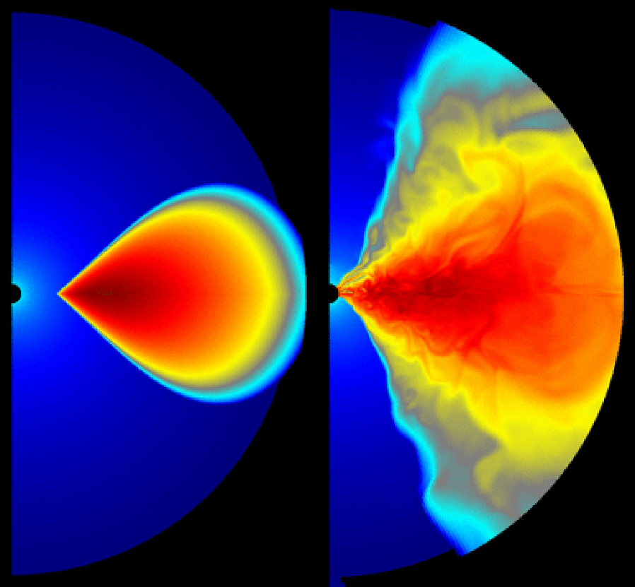
Figure 1: Initial (left) and final (right) distribution of $\log{\rho_{0}}$ in the fiducial model on the $r\sin\theta-r\cos\theta$ plane. At $t=0$ black corresponds to $\rho_{0}\approx 4\times 10^{-7}$ and dark red corresponds to $\rho_{0}=1$. For $t=2000$, black corresponds to $\rho_{0}\approx 4\times 10^{-7}$ and dark red corresponds to $\rho_{0}=0.57$. The black half circle at the left edge is the black hole.

Figure 1 shows the initial and final density states projected on the ($R,z=r\sin{\theta},r\cos{\theta}$)-plane. Color represents $\log(\rho_{0})$. The initial density maximum is $1$ and the minimum is $\approx 4\times 10^{-7}$. The final state contains shocks driven by the interaction with the magnetic field, outflows near the surface of the disk, and an evacuated “funnel” region near the poles.

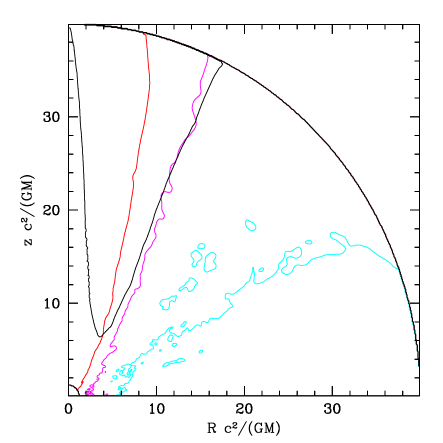
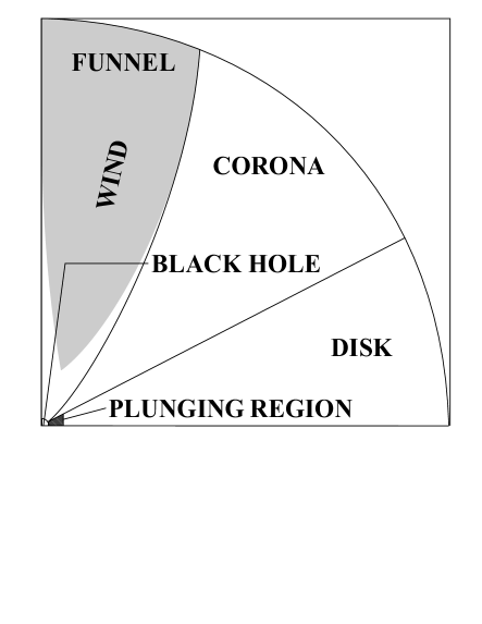
Figure 2: (a) The distribution of $\beta$, $b^{2}/\rho_{0}$, and $u_{t}$ in the fiducial run, based on time and hemispherically averaged data. Starting from the axis and moving toward the equator: (1) $u_{t}=-1$ contour shown as a solid black line; (2) $b^{2}/\rho_{0}=1$ contour shown as a red line; (3) $\beta=1$ contour shown as a magenta line that nearly matches part of the $u_{t}=-1$ contour line; and (4) $\beta=3$ contour is shown as cyan line. (b) Motivated by the left panel, the right panel indicates the location of the five main subregions of the black hole magnetosphere. They are (1) the disk: a matter dominated region where $b^{2}/\rho_{0}\ll 1$; (2) the funnel: a magnetically dominated region around the poles where $b^{2}/\rho_{0}\gg 1$ where the magnetic field is collimated and twists around and up the axis into an outflow; (3) the corona: a region in the relatively low density upper layers of the disk with weak time-averaged poloidal field; (4) the plunging region; and (5) the wind, which straddles the corona-funnel boundary. See section 3.1 for a discussion.

The left panel in figure 2 indicates the relative densities of internal, magnetic, and rest-mass energy. The magenta and cyan contours show the ratio of the average pressure to average magnetic pressure, $\beta\equiv 2\bar{p}/\bar{b^{2}}$. The overbar indicates an average taken over $1000<t<2000$ and over both hemispheres. The cyan contour indicates $\beta=3$ and encircles most of the high density, approximately Keplerian disk. The magenta contour indicates $\beta=1$. The red contour indicates where $\bar{b^{2}}/\bar{\rho_{0}}=1$. Between the pole and this contour the magnetic energy density exceeds the internal and rest-mass energy density. The black contour surrounds a region, extending to large radius, where $-u_{t}>1$ and the flow is directed outward (at large radius $-u_{t}$ asymptotes to the Lorentz factor). That is, the particle energy-at-infinity is larger than the rest-mass density: so the fluid is in a sense, unbound. We use the value of $u_{t}$ to estimate the radial component of the 3-velocity at infinity ($\tilde{v}^{r}$), which is independent of the coordinate system.

The right panel in figure 2 defines some useful terminology inspired by the left panel, following De Villiers & Hawley (2003) and Hirose et al. (2003). Moving from the axis to the equator, the “funnel” is the nearly evacuated, strongly magnetized region ($b^{2}\gg\rho_{0}+u+p$), that develops over the poles. The “wind” consists of a cone of material near the edge of the funnel that is flowing outward with an asymptotic radial velocity of $\tilde{v}^{r}\sim 0.75c$. Near the outer edge of our computational domain the wind becomes marginally superfast. The “corona” lies between the funnel and the disk and has $b^{2}/2\sim p$ except in strongly magnetized filaments. In the “disk” $b^{2}/2<p$ and the plasma follows nearly Keplerian orbits. Finally, the “plunging” region, which lies between the disk and the event horizon, contains accreting material moving on magnetic field and pressure modified geodesics.

Figure 3: Initial (left) and final (right) distribution of $A_{\phi}$. Level surfaces coincide with magnetic field lines and field line density corresponds to poloidal field strength. In the initial state field lines follow density contours if $\rho_{0}>0.2\rho_{0,max}$.

Figure 3 shows the evolution of the poloidal magnetic field. The panels show contours of constant $A_{\phi}$, so the density of contours is directly related to the poloidal field strength, and the contours follow magnetic field lines. The contours are projected on the ($R=r\sin{\theta}$, $z=r\cos{\theta}$)-plane, and show the initial and final state. The initial field is confined to a region much smaller than the torus as a whole because field is introduced only in those portions of the disk that have $\rho_{0}>0.2\rho_{max}$. Notice that by the end of the simulation the field has mixed in to the funnel region and has a regular geometry there. In the disk and at the surface of the disk the field is curved on the scale of the disk scale height. The field strengths and geometries we see are consistent with Hirose et al. (2003). This includes the absence of disk to disk field loops, and that the funnel field collimates instead of connecting back into the disk (thus providing a means for the outflow to escape to large radii).

Figure 4: Contour plot of the time and hemispheric average of $A_{\phi}$. Level surfaces coincide with magnetic field lines and field line density corresponds to poloidal field strength.

Figure 4 shows contours of time and hemisphere averaged $A_{\phi}$. The time averaged field is even more regular in the funnel than the snapshot in Figure 3. Time averaging tends to sharply reduce the field strength in the corona and disk because the field fluctuates in magnitude and direction there.

Figure 5: Evolution of rest-mass, energy, and angular momentum accretion rate for our fiducial run of a weakly magnetized tori around a black hole with spin $a=0.938$. For $500<t<2000$ the time average of these values is ${\dot{M}}_{0}\simeq 0.35$, $\dot{E}/{\dot{M}}_{0}\simeq 0.87$, and $\dot{L}/{\dot{M}}_{0}\simeq 1.46$ as shown by the dashed lines. The dotted lines show the classical thin disk values ($\dot{E}/{\dot{M}}_{0}\simeq 0.82$ and $\dot{L}/{\dot{M}}_{0}\simeq 1.95$). See section 3.1 for a discussion.

Figure 5 shows the accretion rate of rest-mass (${\dot{M}}_{0}$), energy per unit rest-mass ($\dot{E}/{\dot{M}}_{0}$), and angular momentum per unit rest-mass ($\dot{E}/{\dot{M}}_{0}$) evaluated inside the horizon at the inner boundary of the computational domain. For $500<t<2000$ the time average values are ${\dot{M}}_{0}\approx 0.35$, $\dot{E}/{\dot{M}}_{0}\approx 0.87$, and $\dot{L}/{\dot{M}}_{0}\approx 1.46$. These average values are shown as dashed lines. The dotted lines show the classical thin disk values $\dot{E}/{\dot{M}}_{0}\approx 0.82$ and $\dot{L}/{\dot{M}}_{0}\approx 1.95$ obtained by setting these ratios equal to respectively the specific energy and angular momentum of particles on the ISCO. The energy per baryon is therefore slightly above the thin disk value, but the angular momentum per baryon is significantly below the thin disk value.

It may be useful to recast the energy flux in terms of a nominal “radiative efficiency” $\epsilon=1-\dot{E}/{\dot{M}}_{0}$. For the fiducial run $\epsilon=13\%$, which is slightly lower than the thin disk with $\epsilon=18\%$. This is likely due to the high temperature of the flow. On the horizon about $20$% of the energy flux would vanish if we set the internal energy to zero. The corresponding zero-temperature efficiency ($1+u_{t}$) would be 32%.

Figure 6: Electromagnetic energy flux density ${F}^{(EM)}_{E}(\theta)$ on the horizon for the fiducial run, based on time and hemisphere averaged data. The mean electromagnetic energy flux is directed outward. See section 3.1 for a discussion.

The chief object of our study is to measure the electromagnetic luminosity of the hole. The time and hemisphere averaged electromagnetic energy flux on the horizon is shown in figure 6. In the funnel region the energy flux density is outward, as predicted by the force-free model of BZ. We compute other interesting quantities by integrating over the horizon and taking a time average (for technical reasons we are using a less resolved time sampling here than used to make figure 5, but the time averages have fractional differences of only 10%). We find ${\dot{E}}^{(EM)}/{\dot{E}}^{(MA)}=-2.3\%$, where the energies per baryon are ${\dot{E}}^{(EM)}/{\dot{M}}_{0}=-0.018$ and ${\dot{E}}^{(MA)}/{\dot{M}}_{0}=0.77$. It is useful to define the ratio of electromagnetic luminosity to nominal accretion luminosity $\tilde{L}={\dot{E}}^{(EM)}/(-\epsilon{\dot{M}}_{0})$. We find $\tilde{L}=16\%$. Thus while the electromagnetic energy flux is outward, it is a small fraction of the inward material energy flux and the BZ luminosity is small compared to the nominal accretion luminosity.

A control calculation at $a=0$ and a resolution of $256^{2}$ gives ${\dot{E}}^{(EM)}/{\dot{E}}^{(MA)}=0.33\%$ and $\tilde{L}=-6.5\%$, where the energies per baryon are ${\dot{E}}^{(EM)}/{\dot{M}}_{0}=0.0032$ and ${\dot{E}}^{(MA)}/{\dot{M}}_{0}=0.95$. ${\dot{E}}^{(EM)}/{\dot{M}}_{0}>0$ and $\tilde{L}<0$ are as expected, since the outward energy flux must vanish for a nonrotating hole (i.e. the BZ effect is not operating). For our sequence of models the BZ effect does not operate for $a\lesssim 0.5$ (see section 4.1). The matter energy flux ratio may be compared to the thin disk value of ${\dot{E}}^{(MA)}/{\dot{M}}_{0}=0.94$.

3.2 Comparison with BZ

The BZ solution was reviewed in section 2.3. BZ were able to find steady force-free field solutions in the limit that $a\ll 1$. Since the fiducial run has $a=0.938$, we ran a special $a=0.5$ model for comparison with BZ.

The BZ solution was found in the force-free limit, so the first question one might ask is whether any region of the model is force-free. To measure this we recall that in the force-free limit

$${T^{\mu\nu}}_{;\nu}=F^{\mu\nu}J_{\nu}=0.$$ (59)

So when the field is force-free the parameter

$$\zeta=\left|{F^{\mu\nu}J_{\nu}F_{\mu\kappa}J^{\kappa}\over{J_{\mu}J^{\mu}F_{\kappa\lambda}F^{\kappa\lambda}}}\right|$$ (60)

is small compared to 1.

Figure 7: The run of the force-free parameter $\zeta$ for the $a=0.5$ run; when $\zeta\ll 1$ the field is approximately force-free. The parameter has been time and hemisphere averaged. The contours show (beginning from the pole and moving toward the equator) $\zeta=10^{-3},10^{-2},10^{-1}$. The small closed contours at large radius and close to the axis have $\zeta=10^{-2}$. The small closed contours from the equator to $\theta\sim\pi/4$ have $\zeta=10^{-1}$. See section 3.2 for a discussion.

Figure 7 shows the time and hemispherical averaged $\zeta(r,\theta)$ from $t=1000$ to $t=2000$ for the $a=0.5$ model. The contours show (beginning from the pole and moving toward the equator) $\zeta=10^{-3},10^{-2},10^{-1}$. The entire funnel region has $\zeta<10^{-2}$ and is therefore effectively force-free. This is true in both a time-averaged and instantaneous sense in the funnel for all our runs. This opens the possibility that the BZ solution describes the funnel.

Figure 8: Left panel: Magnetic field angular frequency on the horizon relative to black hole rotation $\omega(\theta)/\Omega_{H}$. The solid line indicates time and hemisphere averaged data from our $a=0.5$ MHD integration. The middle dotted line is the prediction of the BZ model ($\omega/\Omega_{H}=1/2$). The dashed line (top) is the value predicted by the inflow model. Right panel: the run of field rotation frequency $\omega$ with radius along a single field line that intersects the horizon at $\theta=0.2$. $\omega$ is constant to within 3%, as expected for a steady flow. See sections 3.2 and 3.3 for a discussion.

Figure 9: (a) Square of radial field ($({B^{r}}(\theta))^{2}$) on the horizon in the $a=0.5$ MHD integration, from time and hemisphere averaged data. Solid line is the field for our numerical model. The dotted line shows the Blandford & Znajek (1977) perturbed monopole solution with the field strength normalized to the numerical solution at the pole. The dashed line is the inflow solution. (b) Electromagnetic energy flux ${F}^{(EM)}_{E}(\theta)$ on the horizon in the $a=0.5$ MHD integration, from time and hemisphere averaged data. The solid line shows the numerical model, the dotted line shows BZ’s spun-up monopole solution, and the dashed line shows the inflow solution. See sections 3.2 and 3.3 for a discussion.

A key feature of the BZ model is that the field rotation frequency $\omega\approx\Omega_{H}/2$ for $a\ll 1$ if the field has a monopole geometry. Figure 8a shows the ratio $\omega/\Omega_{H}$ on the horizon. Within the force-free region, which runs from $0<\theta<0.4$ on the horizon, the average $\omega/\Omega_{H}\approx 0.45$. The small difference from the BZ could be due to higher order terms in the expansion in $a$, but Komissarov (2001) has integrated the equations of force-free electrodynamics for a monopolar field geometry and at $a=0.5$ finds that $\omega$ rises from $\approx 0.495\Omega_{H}$ at the pole to $\approx 0.51\Omega_{H}$ at the equator, so this seems unlikely. The difference is more likely due to small deviations from force-free behavior (mass loading of field lines by the numerical “floor” on the density).

In an axisymmetric steady state both the force-free equations and the MHD equations predict that the rotation frequency $\omega$ (and other quantities) are constant along field lines. Figure 8b shows the variation of $\omega$ with radius along a field line that intersects the horizon at $\theta=0.33$. As expected $\omega\approx const.$, with a variation of less than 3% from maximum to minimum.

BZ’s spun-up monopole model makes definite predictions about the variation of $B^{r}$ and ${F_{E}}$ on the horizon. Figure 9a shows the variation in time and hemisphere averaged $(B^{r})^{2}$ and compares to BZ’s monopole field calculation. The single adjustable parameter of the model normalizes the field strength. We have set this normalization by requiring that $(B^{r})^{2}$ match at the pole. Evidently the variation matches the BZ prediction closely even well outside the force-free region at $\theta\approx 1.1$. Figure 9b shows the variation in radial energy flux on the horizon as predicted by the BZ model using the pole-normalized field. Here the match is quite close out to $\theta\approx\pi/4$. It is slightly surprising that the BZ solution does so well even in regions that are not force-free. This is likely a result of trans-field force balance and geometry controlling the distribution of field on the horizon and hence the radial energy flux.

To summarize: in our low spin numerical experiment the funnel is approximately force-free within the funnel. It is approximately in a steady state and hence $\omega$ is approximately constant along field lines. Furthermore, $\omega$, $B^{r}$, and the radial electromagnetic energy flux are all in good agreement with the spun-up monopole force-free model on the horizon. We have not compared the entire funnel region with the monopole model because the field is collimated there and not well described by the monopole solution.

3.3 Comparison to Inflow Solution

The inflow solution of Gammie (1999) considers a near-equatorial stationary MHD inflow in the plunging region, reviewed in section 2.4. Here we compare the inflow models with the fiducial model. Unlike the funnel, the plunging region is rapidly fluctuating, so we expect the inflow model to match only the time-averaged data from the simulation.

The inflow model has two free parameters: the field strength and the accretion rate. The field strength we match by finding the parameter that gives the best fit to the mean magnetic energy density between the ISCO and the event horizon. The rest-mass flux is chosen to agree with the time-averaged data from the simulation. The ratio of the field strength to the square root of the accretion rate is a dimensionless parameter that controls the solution; in the units of Gammie (1999), where $2\pi\rho_{0}u^{r}{\sqrt{-g}}=-1$, we use $F_{\theta\phi}=1.09$ for the comparison model.

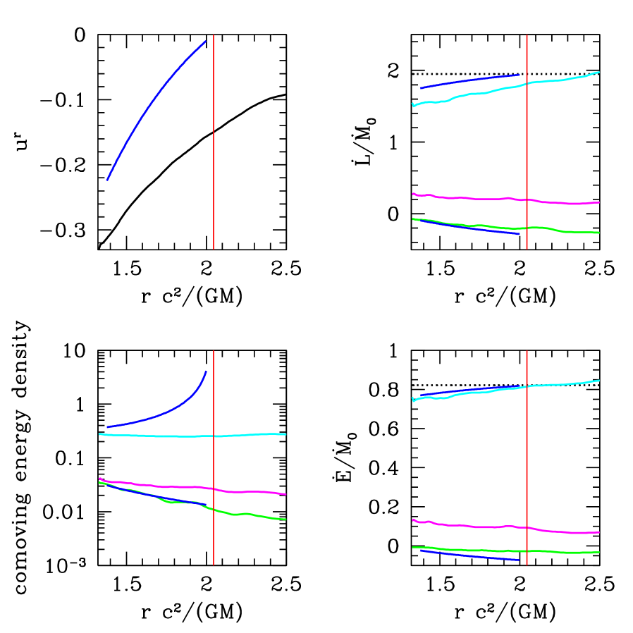
Figure 10: A comparison of the time-averaged fiducial model near the equator (within $\theta=\pi/2\pm 0.3$) with the inflow solution of Gammie (1999). In the right two panels the black dotted line is the thin disk value. In all cases the red vertical line is the location of the ISCO. The black line for the upper left panel is the numerical result. For the other three panels, the particle term is shown in cyan, the internal energy term is shown in magenta, and the electromagnetic term is shown in green. The blue line in each plot represents the inflow model result. Notice that the run of density with radius shows no feature at the ISCO. See the Section 3.3 for discussion.

Figure 10 shows a comparison of $u^{r}$, $\dot{L}/{\dot{M}}_{0}$, comoving energy densities ($\rho_{0}$, $b^{2}/2$, and $u$), and energy fluxes ($\dot{E}/{\dot{M}}_{0}$) in the inflow solution. The comparison data from the fiducial run has been averaged over $|\theta-\pi/2|<0.3$ and $500<t<2000$. Each panel in the figure contains a vertical line at the ISCO.

The upper left panel compares the radial component of the four-velocity (in KS and BL coordinates) in the inflow and numerical solutions. The substantial differences are due to the finite temperature of the flow; the inflow solution is cold by assumption. Radial pressure gradients in the numerical model (which are absent in the inflow solution) begin to accelerate material inward outside the ISCO, and the flow becomes supersonic near the ISCO.

The upper right and lower right panels show components of the energy and angular momentum flux from the simulation and inflow solutions. The dashed horizontal line in each case shows the values expected for a thin disk; the inflow solution is constrained to match the thin disk at the ISCO. The cyan lines show $u_{\phi}$ (upper panel) and $u_{t}$ (lower panel) from the simulation, while the blue lines show the prediction from the inflow model. The energy flux matches rather well (although notice that this is only a small fraction of the energy flux), while the angular momentum is overestimated; in the simulation the plasma has sub-Keplerian angular momentum by the time it reaches the ISCO.

The electromagnetic components of the normalized angular momentum flux ($b^{2}u_{\phi}/\rho_{0}-b^{r}b_{\phi}/(\rho_{0}u^{r})$) and energy flux ($b^{2}u_{t}/\rho_{0}-b^{r}b_{t}/(\rho_{0}u^{r})$) are also shown in the upper and lower right panels of figure 10 (green line $\equiv$ simulation, blue line $\equiv$ inflow solution). The inflow solution matches well, although it tends to overestimate the magnitude of the outward directed energy flux.

The magenta lines in the upper and lower right panels show the internal energy component of the normalized angular momentum flux ($(u+p)u_{\phi}/\rho_{0}$) and energy flux ($-(u+p)u_{t}/\rho_{0}$). This component of the fluxes is zero by assumption in the inflow solution, and it is evidently an important component of the fluxes in our thick disk simulations. This leads to large corrections to the angular momentum and energy fluxes; the total normalized angular momentum flux is significantly smaller than the thin disk prediction, while the energy flux is, seemingly by conspiracy, very close to the thin disk.

The lower left panel shows the rest-mass density from the inflow solution (upper blue line) and from the simulation (cyan line). The mass flux in the inflow solution is normalized so that it matches the simulation mass flux. Since mass flux is approximately constant with radius, the run of density is directly related to the run of $u^{r}$. What is remarkable here is that there is no feature in the simulation $\rho_{0}$ near the ISCO. In fact it is nearly constant from well outside the ISCO in to the event horizon. The surface density varies smoothly as well. This confirms the point made by Krolik & Hawley (2002) in their pseudo-Newtonian solution: there is no sharp feature at the ISCO. This has implications for iron line profiles, as discussed by Reynolds & Begelman (1997).

The lower left panel also shows the run of internal energy density in the simulation (it is zero by assumption in the inflow solution). Again, there is no sharp feature at the ISCO, just a gentle rise inward toward the event horizon. Because the density is nearly constant with radius this implies that entropy is increasing inward. Therefore there is some dissipation of kinetic or magnetic energy into internal energy in the inflow region.

The lower left panel of figure 10 shows the run of magnetic energy density $b^{2}/2$ in the inflow solution (lower blue line) and simulation (green line). The normalization of the inflow magnetic energy is a parameter, but its radial slope is not.

Finally, the inflow solution predicts that $\omega=\Omega_{ISCO}$. Figure 8a shows the run of $\omega/\Omega_{H}$ on the horizon for the $a=0.5$ model. The dashed line shows the ISCO value of $\omega/\Omega_{H}$. At the equator the time-averaged numerical value lies within about $10\%$ of the ISCO value: the numerical average $\omega/\Omega_{H}=0.685$, while the $\Omega_{ISCO}/\Omega_{H}=0.8136$ at the ISCO. In the $a=0.938$ run the numerical average $\omega/\Omega_{H}=0.681$, while $\Omega_{ISCO}/\Omega_{H}=0.745$ at the ISCO.

To sum up, the inflow model does a surprisingly good job of matching some aspects of the time-averaged simulation. It does not match the profile or boundary condition at the ISCO for the radial velocity or the total angular momentum and energy fluxes, because the simulation flow is hot, while the inflow solution has zero temperature by assumption.

What is most surprising is that the energy per baryon accreted in the numerical model matches the thin disk prediction. The inflow model predicts that the energy per baryon accreted should be lower than the thin disk prediction, enhancing the nominal accretion efficiency (Gammie, 1999; Krolik, 1999; Agol & Krolik, 2000). The difference is apparently due to the finite temperature of the numerical model and the consequent change in boundary conditions at the ISCO. These boundary conditions evidently adjust themselves to maintain the energy flux at the thin disk value. The angular momentum flux is affected by the field, however, with the specific angular momentum of the accreted material in the fiducial run about $25\%$ lower than the thin disk.

4 Parameter Study

Our numerical model has a number of physical and numerical parameters. Here we check the sensitivity of the model to: (1) black hole spin parameter $a$; (2) initial magnetic field geometry and initial magnetic field strength; and (3) numerical parameters such as (a) location of the inner boundary ($R_{in}$); (b) outer radial ($R_{out}$) boundary; (c) radial and $\theta$ resolution, including the coordinate parameter $h$; and (d) parameters describing the density and internal energy floors.

4.1 Black Hole Spin

The fiducial run has a rather low outgoing electromagnetic energy flux compared to the ingoing matter energy flux. It is possible that this varies sharply with black hole spin and that more rapidly rotating holes exhibit much larger electromagnetic luminosity. We have performed a survey over $a$, keeping all parameters identical to those in the fiducial run, except that the resolution is lowered to $256^{2}$ and the location of the pressure maximum is adjusted to keep $H/R\approx const$.

Figure 11: The ratio of electromagnetic to matter energy flux on the horizon. The solid line indicates numerical data while the dotted line indicates a best fit of ${\dot{E}}^{(EM)}/{\dot{E}}^{(MA)}=-0.068(2-r_{+})^{2}$. See section 4.1 for a discussion.

Table 2: Black Hole Spin Study

$a$	$10^{4}\times{\dot{E}}^{(EM)}/{\dot{E}}^{(MA)}$	$\dot{E}/{\dot{M}}_{0}$	$\dot{L}/{\dot{M}}_{0}$	$\dot{a}/{\dot{M}}_{0}$	${\dot{M}}_{0}$	$\tilde{L}$
-0.938	105	0.958	3.806	-5.583	-0.908	-0.24
0.000	34.4	0.950	3.068	-3.049	-0.870	-0.065
0.050	31.2	0.952	3.025	-2.921	-0.709	-0.062
0.100	35.8	0.948	2.896	-2.713	-0.767	-0.066
0.150	29.7	0.949	2.881	-2.597	-0.796	-0.055
0.200	26.9	0.948	2.817	-2.439	-0.776	-0.050
0.250	9.17	0.946	2.749	-2.302	-0.747	-0.016
0.300	3.30	0.937	2.759	-2.217	-0.571	-0.0049
0.350	1.32	0.933	2.605	-1.975	-0.620	-0.0018
0.400	1.15	0.937	2.763	-1.986	-0.241	-0.0017
0.500	-9.85	0.933	2.583	-1.665	-0.252	0.014
0.600	-28.5	0.929	2.489	-1.347	-0.318	0.037
0.750	-81.8	0.908	2.150	-0.808	-0.276	0.083
0.875	-291	0.852	1.440	-0.152	-0.170	0.17
0.895	-254	0.891	1.723	-0.204	-0.215	0.20
0.900	-315	0.882	1.674	-0.118	-0.193	0.24
0.938	-318	0.856	1.396	0.067	-0.203	0.23
0.969	-410	0.869	1.374	0.217	-0.172	0.27

Note. — All models same as fiducial except at a resolution of $256^{2}$ and $r_{max}$ is used to keep $H/R\sim constant$. These values can be compared to Tables 3 and 4. The efficiency is $1-\dot{E}/{\dot{M}}_{0}$. A positive $\dot{a}/{\dot{M}}_{0}$ corresponds to a spindown of the black hole since ${\dot{M}}_{0}<0$.

The results are shown in figure 11 and described in table 2. The figure shows the measured ratio of electromagnetic to rest-mass energy flux; the dashed line shows a fit

$$\frac{{\dot{E}}^{(EM)}}{{\dot{E}}^{(MA)}}\approx-0.068(2-r_{+})^{2}.$$ (61)

This fit applies only to this particular sequence of models; models with different initial field geometries give different results, as we shall see below. For all $a>0$ we find ${\dot{E}}^{(EM)}>0$ in the funnel. For $a<0.5$ this outward funnel flux is balanced by an inward electromagnetic energy flux near the equator. For our most extreme run with $a=0.969$ the outward electromagnetic flux is still dominated by the inward particle flux. The ratio of electromagnetic luminosity to nominal accretion luminosity is $\tilde{L}=27\%$, so the nominal accretion luminosity dominates over the BZ luminosity.

The accretion rate of angular momentum is also a strong function of spin. As discussed in Gammie, Shapiro, & McKinney (2004), accretion flows around rapidly spinning holes have $da/dt<0$. Our fiducial model, in fact, is spinning down. Previous estimates suggested that spin equilibrium is reached at $a\sim 0.998$ (Thorne, 1974). Our models reach spin equilibrium at $a\sim 0.92$.

The variation of field strength and geometry with black hole spin is also of interest. To measure variation of field strength, we probe the flow near four locations: 1) in the funnel near the horizon (“funnel/horizon”); 2) in the plunging region near the horizon (“plunging/horizon”); 3) at the ISCO; and 4) at the pressure maximum. We then take a time and spatial average of the comoving electromagnetic energy density $b^{2}/2$ over a small region near each of these locations. The ratio of $b^{2}$(funnel/horizon) to $b^{2}$(plunging/horizon) changes from $0.43$ at $a=0$ to $0.74$ at $a=0.938$. The ratio of $b^{2}$(funnel/horizon) to $b^{2}$(ISCO) varies from $2.53$ at $a=0$ to $2.14$ at $a=0.938$. The ratio $b^{2}$(funnel/horizon) to pressure maximum varies from $4.8$ at $a=0$ to $15.7$ at $a=0.938$. In summary, the field strength increases from the ISCO to the horizon by a factor of $\sim 3$ at $a=0$ and by a factor of $\sim 6$ at $a=0.938$, and on the horizon is slightly larger at the equator than at the poles by a factor of $\sim 2$. Only the ratio of $b^{2}$(pressure maximum) to other locations in the plunging region or at the horizon depends strongly on black hole spin.

Our observed increase in horizon field strength with black hole spin agrees with results reported by De Villiers, Hawley, & Krolik (2003). We see no sign of the expulsion of flux from the horizon reported by Bicak & Janis (1985), who find that the flux through one hemisphere of the horizon, due to external sources and calculated in axisymmetry using vacuum electrodynamics, vanishes when the spin of the hole is maximal. It is possible that we have not gone close enough to $a=1$ to observe this effect.

To investigate the variation of field geometry in the funnel region with $a$ we trace field lines from $\theta_{in}$ on the horizon to $\theta_{out}$ on the outer boundary and define a collimation factor $\theta_{in}/\theta_{out}$. The collimation factor is similar for all field lines in the funnel region. It reaches a minimum of $\approx 5/2$ for the fiducial run, and rises to nearly $2$ for $a=0$ and again to nearly $2$ for $a\sim 1$. The collimation factor depends on the location of the outer boundary; for models with $R_{out}=400$ the collimation factor is $10$ and the field lines are nearly cylindrical at the outer boundary.

We have also studied the variation of the field rotation frequency $\omega$ in the funnel. $\omega/\Omega_{H}$ varies weakly with $a$, from $0.53$ at $a=0.25$ to $0.45$ at $a=0.938$, consistent with the hypothesis advanced by Thorne, Price, & MacDonald (1986) that $\omega/\Omega_{H}\approx 1/2$.

4.2 Field Geometry and Strength

The outcome of the simulation may also depend on the field geometry and strength in the initial conditions. This seems more likely for axisymmetric models such as ours where the evolution may retain a stronger memory of the initial conditions than comparable three dimensional models.

Table 3: Field Strength and Geometry Study

Field Geometry $A_{\phi}$	$\beta$	${\dot{E}}^{(EM)}/{\dot{E}}^{(MA)}$	$\dot{E}/{\dot{M}}_{0}$	$\dot{L}/{\dot{M}}_{0}$	$\dot{a}/{\dot{M}}_{0}$	${\dot{M}}_{0}$	$\tilde{L}$
$A^{0}_{\phi}$	$100$	$-0.0312$	$0.856$	$1.40$	$0.0674$	$-0.203$	$0.21$
$A^{0}_{\phi}$	$500$	$-0.0115$	$0.879$	$1.94$	$-0.293$	$-0.0474$	$0.085$
$A^{0}_{\phi}\sin{(\log{(r/h)})}$	$100$	$-0.0355$	$0.892$	$1.24$	$0.278$	$-0.541$	$0.42$
$A^{0}_{\phi}|\sin(2\theta)|$	$100$	$-0.0112$	$0.888$	$1.91$	$-0.299$	$-0.0746$	$0.083$
$r\sin{\theta}$	$100$	$-0.147$	$0.773$	$-0.997$	$1.807$	$-1.769$	$0.79$
$r\sin{\theta}$	$400$	$-0.157$	$0.813$	$0.0617$	$1.184$	$-0.715$	$0.67$

Note. — $A^{0}_{\phi}$ is the fiducial model field geometry and $\beta=100$ is the fiducial ratio of gas to magnetic pressure. The $r\sin{\theta}$ field geometry is a uniform vertical field model with $\beta$ set by disk values at the equator. All other model and numerical parameters are as in the fiducial model except that the resolution is $256^{2}$. The efficiency is $1-\dot{E}/{\dot{M}}_{0}$. A positive $\dot{a}/{\dot{M}}_{0}$ corresponds to a spindown of the black hole because ${\dot{M}}_{0}<0$.

We begin by investigating the dependence of outcome on initial field strength, parameterized by $\beta\equiv p_{gas,max}/p_{mag,max}$ (notice that the two maxima never occur at the same location in space, so this ratio varies over a wide range when evaluated at individual locations in the disk). We consider models with $\beta=(100,500)$ and find a weak dependence on $\beta$. For the $\beta=100$ model (the fiducial model at a resolution of $256^{2}$) we find $\omega/\Omega_{H}\approx 0.45$, ${\dot{E}}^{(EM)}/{\dot{E}}^{(MA)}\approx-3.1\%$, and $\tilde{L}=21\%$. $\beta=500$ leads to $\omega/\Omega_{H}\approx 0.42$, ${\dot{E}}^{(EM)}/{\dot{E}}^{(MA)}=-1.2\%$, and $\tilde{L}=8.5\%$. Notice that a higher spatial resolution is required to fully resolve weak field models, although all runs in this comparison were done at $256^{2}$; the decrease in electromagnetic energy extracted at $\beta=500$ may therefore be due to resolution.

We also vary the field geometry from the single loop used in our fiducial model, which has vector potential $A_{\phi}\propto MAX(P/P_{max}-0.2,0)$. We do this by multiplying the vector potential by $\sin(\log(r/h))$ or $|\sin(2\theta)|$. The former decompresses the field lines at the inner radial edge giving a field strength that is more uniform around the loop (for an extended disk this would yield a sequence of field loops centered at the midplane with alternating sense of circulation). The latter yields two loops, one centered above the equator and the other below, with the same sense of circulation. The $\sin(\log(r/h))$ modulation gives $\omega/\Omega_{H}\approx 0.44$, ${\dot{E}}^{(EM)}/{\dot{E}}^{(MA)}\approx-3.6\%$, and $\tilde{L}=42\%$. The $|\sin(2\theta)|$ modulation gives $\omega/\Omega_{H}\approx 0.40$, ${\dot{E}}^{(EM)}/{\dot{E}}^{(MA)}\approx-1.1\%$, and $\tilde{L}=8.3\%$. Increasing the number of initial field loops therefore leads to a weak (factor of $2-3$) decrease in ${\dot{E}}^{(EM)}/{\dot{E}}^{(MA)}$, while making the field strength more uniform around the loop increases $\tilde{L}$ by a factor of $2$ with a nearly constant ${\dot{E}}^{(EM)}/{\dot{E}}^{(MA)}$. Higher resolution studies may better resolve these simulations and show weaker dependence on field geometry.

We have also considered a purely vertical field geometry: $A_{\phi}\propto r\sin\theta$. In a Newtonian context this would correspond to a uniform $z$ field in cylindrical coordinates. The field is normalized so that $\beta=p_{gas,max}/p_{mag,max}=100$ and $400$ in the equator of the torus. The outcome is different from any of the other models.

The funnel field in the vertical field run is strong compared to the disk field. The accretion rate is larger, by a factor of $5$, than the fiducial run. In the early stages there is a brief net outflow of energy from the black hole (although the total energy released from the hole is negligible compared to the energy gained at later times). The $\beta=100$ model has a high mean efficiency; $\dot{E}/{\dot{M}}_{0}=0.77$, compared to $0.82$ expected for a thin disk. There is also a net outflow of angular momentum from the black hole, with $\dot{L}/{\dot{M}}_{0}=-1.00$, compared to $1.95$ expected for a thin disk. The wind has a peak asymptotic radial velocity $\tilde{v}^{r}=0.94c$, attained near the outer boundary, compared to $\tilde{v}^{r}=0.75c$ for the fiducial run. Finally, the model has $\omega/\Omega_{H}\approx 0.41$, ${\dot{E}}^{(EM)}/{\dot{E}}^{(MA)}\approx-15\%$, and $\tilde{L}=79\%$. The $\beta=400$ vertical field model has very similar properties, which suggests that we are resolving the $\beta=100$ model. Table 3 summarizes measurements from the varying field geometry models.

The models with net vertical field exhibit markedly different behavior from the fiducial model. It seems likely that some of this difference is due to the axisymmetric nature of the model; in 3D matter can accrete between the vertical field lines without having to push them into the hole. That is, in 3D, it would be easier for the hole to rid itself of the dipole moment that it acquires in the net vertical field calculation. But we cannot say with any confidence what the outcome is until a full 3D experiment on a disk with nonnegligible magnetic dipole moment.

4.3 Numerical Parameters

Table 4: Resolution Study

Resolution	${\dot{E}}^{(EM)}/{\dot{E}}^{(MA)}$	$\dot{E}/{\dot{M}}_{0}$	$\dot{L}/{\dot{M}}_{0}$	$\dot{a}/{\dot{M}}_{0}$	${\dot{M}}_{0}$	$\tilde{L}$
$64^{2}$	-0.0528	0.914	1.630	0.036	-0.159	0.55
$128\times 64$	-0.0438	0.841	1.420	0.121	-0.165	0.23
$128^{2}$	-0.0447	0.887	1.518	0.087	-0.167	0.38
$256^{2}$	-0.0316	0.874	1.274	0.198	-0.186	0.27
$456^{2}$	-0.0261	0.865	1.381	0.216	-0.299	0.18

Note. — Numerator and denominators are separately time averaged from $500<t<1000$ at the horizon. This interval is chosen so that all models are turbulent (in the lowest resolution model turbulence decays shortly after $t=1000$). The $456^{2}$ model is the fiducial model. The nominal radiative efficiency is $1-\dot{E}/{\dot{M}}_{0}$. A positive $\dot{a}/{\dot{M}}_{0}$ corresponds to a spindown of the black hole because ${\dot{M}}_{0}<0$.

We have run the fiducial model at resolutions of $64^{2}$, $128^{2}$, $128\times 64$, $256^{2}$, and $456^{2}$. There is a weak dependence on resolution in the sense that ${\dot{E}}^{(EM)}/{\dot{E}}^{(MA)}$ is smaller at higher resolutions. Lower resolution models do not sustain turbulence for as long as high resolution models, so we average over $500<t<1000$, when all models are turbulent. Table 4 gives a summary of results from the resolution study. In every case the nominal radiative efficiency is close to the thin disk value.

Resolution of the near-horizon region, where the energy density is large, is also a concern, because our accretion rates are measured there. We have checked dependence on radial numerical resolution of the near-horizon region by modifying the coordinate definition in equation (7) to read $r=R_{0}+e^{x_{1}}$ rather than $r=e^{x_{1}}$. Increasing $R_{0}$ from $0$ to the horizon radius increases the number of grid zones located near the horizon. We ran a model with $R_{0}=0.5$ and found no significant difference from a comparable model with $R_{0}=0$. This suggests that we are adequately resolving the near-horizon region.

We also varied $R_{in}$ and $R_{out}$ and found no measurable difference in ${\dot{E}}^{(EM)}$, ${\dot{E}}^{(MA)}$, $(B^{r})^{2}$, and $\omega$ on the horizon. We have moved $R_{out}$ from $40$ to $400$ and $R_{in}$ from $0.7r_{+}$ to $0.98r_{+}$ and find negligible differences in these quantities on the horizon. The solution is not sensitive to the location of the inner or outer boundary. Moving the inner boundary of the computational domain outside the horizon (e.g. $1.05r_{+}$) leads to strong reflections from the boundary conditions and, ultimately, failure of the run. It is possible that better inner boundary conditions or higher resolutions could overcome this difficulty, but it seems cleaner to simply leave the boundary inside the event horizon at $r=0.98r_{+}$, out of causal contact with the rest of the simulation.

The model with larger $R_{out}=400$ does exhibit some new features. The magnetic field lines in the funnel region have a collimation factor of $10$ by the time they reach the outer boundary. At $R=40$, however, both the $R_{out}=400$ model and the fiducial model have a collimation factor of $5/2$. By $R_{out}=400$ the field lines are nearly cylindrical. The peak of the radial component of the asymptotic 3-velocity in the wind is identical to the fiducial run with $\tilde{v}^{r}=0.75c$, indicating little acceleration between $R=40$ and $R=400$.

The main numerical uncertainty in our experiments arise from the floor on the density and internal energy. We varied the floor scaling from $\rho_{0,min}=10^{-4}r^{-3/2}$ and $u_{min}=10^{-6}r^{-5/2}$ to $\rho_{0,min}=10^{-4}r^{-2.7}$ and $u_{min}=10^{-6}r^{-3.7}$ (we chose these scalings so that $b^{2}/\rho_{0}$ would be nearly constant with radius in the funnel). While this significantly affects $b^{2}/\rho_{0}$, it does not otherwise affect ${\dot{E}}^{(EM)}$ and ${\dot{E}}^{(MA)}$ or the mean values of $B^{r}$ and $\omega$ measured on the horizon.

We varied the floor normalization at $r=1$ from the fiducial values $(\rho_{0,min},u_{min})=(10^{-4},10^{-6})$ to $(10^{-5},10^{-7})$, and $(10^{-6},10^{-8})$. This causes almost no change in the flow near the horizon. In the funnel, however, we are at the limit of our ability to integrate the MHD equations ($b^{2}/\rho_{0}\gg 1$). Our integration fails when we attempt to use a mass density floor $\rho_{0,min}(r=1)\lesssim 10^{-5}$ when $R_{out}\gg$ the outer edge of the initial torus. Lower floors lead to faster outflows $\tilde{v}^{r}\gg 0.99c$ in the funnel region, which are more likely to be numerically unstable. These results hint that low density models will produce fast outflows, but a confirmation awaits a more stable GRMHD algorithm.

The funnel region is difficult to integrate reliably, because when $b^{2}/\rho_{0}\gg 1$ small fractional errors in field evolution lead to large fractional errors in the evolution of other flow variables. This is a consequence of our conservative scheme, in which all the dependent variables are coupled together by the interconversion of primitive and conserved variables. Evolution of the MHD equations in nonconservative form (e.g. using an internal, rather than total, energy equation), as in De Villiers & Hawley (2003), may be slightly more robust, although De Villiers and Hawley eventually experience similar problems in the funnel. In any event, the close correspondence between the numerical experiment and the BZ model raises confidence in the results and suggests that the magnetic field, if not the mass density and internal energy density, is being evolved reliably.

5 Discussion

We have used a general relativistic MHD code, HARM, to evolve a weakly magnetized thick disk around a Kerr black hole. Our main result is that we find an outward electromagnetic energy flux on the event horizon, as anticipated by Blandford & Znajek (1977). The funnel region near the polar axis of the black hole is consistent with the Blandford-Znajek model. The outward electromagnetic energy flux is, however, overwhelmed by the inward flux of energy associated with the rest-mass and internal energy of the accreting plasma. This result essentially confirms work by Ghosh & Abramowicz (1997); Livio, Ogilvie, & Pringle (1999) that suggested the BZ luminosity should be small or comparable to the nominal accretion luminosity ($\tilde{L}\lesssim 1$).

One of our models discussed here, however, begins with a vertical field threading the torus, exhibits a brief episode of outward net energy flux. This appears to be a transient associated with the initial conditions. The same model exhibits a steady net outflow of angular momentum from the black hole. Of all our models, the vertical field model has the largest negative $-{\dot{E}}^{(EM)}/{\dot{E}}^{(MA)}\approx 15\%$ (ratio of the electromagnetic energy flux to ingoing matter energy flux) and largest $\tilde{L}={\dot{E}}^{(EM)}/(-\epsilon{\dot{M}}_{0})\approx 80\%$ (ratio of electromagnetic luminosity to nominal accretion luminosity). This suggests that the BZ effect could play a significant role if the disk has a net dipole moment and accumulates magnetic flux that crosses the horizon. This possibility will be considered in future work.

Consistent with the results found earlier by De Villiers, Hawley, & Krolik (2003), we find that our models can be divided into four regions: (1) a “funnel” region with $b^{2}/\rho_{0}\gtrsim 1$ and $\beta\ll 1$; (2) a corona with $1\lesssim\beta\lesssim 3$; (3); an equatorial disk with $\beta>3$; and (4) a plunging region between the disk and event horizon with $\beta\sim 1$ and a nearly laminar inflow from the disk to the black hole. We also find no feature in the surface density at or near the ISCO (see figure 10), which agrees with the results by Krolik & Hawley (2002); De Villiers, Hawley, & Krolik (2003) and consistent with Reynolds & Begelman (1997). This is contrary to the sharp transition predicted by thin disk models and used by XSPEC to fit X-ray spectra.

We have shown that the funnel region is nearly force-free, and is well described by the stationary force-free magnetosphere model of Blandford & Znajek (1977), for which we have presented a self-contained derivation in Kerr-Schild coordinates. We find agreement between the BZ model and our simulations in measurements of energy flux, magnetic field, efficiency of accretion, and spindown power output. In all cases we find that in the force-free region the field rotation frequency is about half the black hole spin frequency, $\Omega_{H}\equiv a/(2r_{+})$. This spin frequency maximizes electromagnetic energy output from the hole. This result is consistent with expectations of MacDonald & Thorne (1982b) and the force-free numerical results of Komissarov (2001).

We have also compared the time-average of the plunging region in our fiducial model with the stationary MHD inflow model of Gammie (1999), which assumes that the flow matches a cold disk at the ISCO. The inflow model matches the simulated rest-mass flux and electromagnetic flux of energy and angular momentum surprisingly well, particularly considering the strongly variable nature of the simulated flow in the plunging region. The inflow model fails to match other aspects of the flow, such as the radial component of the four-velocity. This is mainly due to the finite temperature of the simulated flow; the inflow solution assumes zero temperature. It is slightly surprising that the total angular momentum flux is close to the value predicted by the zero temperature inflow solution, and $20\%$ less than what is predicted by the thin disk, yet the total energy flux is almost exactly what is predicted by the thin disk. It is as yet unclear whether this is due to coincidence or conspiracy.

For a set of models similar to the fiducial model, the ratio of electromagnetic to matter energy fluxes is sensitive to the black hole spin, reaching $-7\%$ for $a\sim 1$. The evolution is sensitive to the initial field geometry. Models with a net vertical field are more efficient, and more electromagnetically active than models with comparable field strength but zero net vertical field. Our models have a weak dependence on resolution in the sense that as resolution increases the relative importance of electromagnetic energy fluxes on the horizon diminishes.

With an $R_{out}=400$ model we demonstrate that an outgoing electromagnetic energy flux can reach large radii. The field in the funnel region does not connect back into the disk. Rather the poloidal components lie parallel to the polar axis. The field lines are collimated by a factor of $5/2$ at $r=40$ and by a factor of $10$ at $r=400$. An outflow along the boundaries of the funnel reaches a maximum $\tilde{v}^{r}\approx 0.75c$, but this is sensitive to the value of our artificial density “floor”: a model with lower density reaches even larger radial velocities at the outer boundary of the computational domain.

Koide, Shibata, Kudoh, & Meier (2002) have evolved a cold, highly magnetized uniform density plasma ($\rho_{0}/p=0.06$, $b^{2}/\rho_{0}=10$) as it falls into a rapidly spinning ($a=0.99995$) black hole in Boyer-Lindquist coordinates for a time $\approx 14GM/c^{3}$ using the MHD approximation. This initial state does not correspond to an accretion disk system. They demonstrated, however, that a transient net energy extraction is possible from a spinning black hole. Because of the short evolution time they are unable to say whether the energy extraction process is possible in steady state. Koide (2003) gives an expanded discussion of the above system.

In contrast to the results of Koide, Shibata, Kudoh, & Meier (2002) and Koide (2003), we model a disk with an initially hydrodynamic equilibrium fluid that is weakly magnetized. We also use a Kerr-Schild (horizon penetrating) coordinate system that avoids potential problems associated with the treatment of inner boundary condition in Boyer-Lindquist coordinates. In our simulation the Balbus-Hawley instability drives turbulence and accretion in a steady state where we evolve for a time $2000GM/c^{3}$. We measure a sustained outward electromagnetic energy flux that is smaller than the inward matter energy flux (i.e. net inward energy flux). Their model is evolved for too short a time to observe the unbound mass outflow in the funnel region as seen by us and De Villiers, Hawley, & Krolik (2003); De Villiers & Hawley (2004).

De Villiers & Hawley (2004)(hereafter DH) have also considered the numerical evolution of weakly magnetized tori around rotating black holes. Their models are quite similar to ours in many respects, although they differ in that: (1) their models are three dimensional while our models are axisymmetric; (2) they use a nonconservative numerical method De Villiers & Hawley (2003); (3) DH use Boyer-Lindquist while we use Kerr-Schild coordinates; (4) DH choose $\gamma=5/3$ while we use $\gamma=4/3$; (5) DH’s initial pressure maximum is located at $25M$, while ours are typically at $12M$. Our results for the energy and angular momentum per baryon accreted from table 2 can be compared to Table 1 of DH by computing $\dot{E}/{\dot{M}}_{0}=\Delta E_{i}/\Delta M_{i}$ and $\dot{L}/{\dot{M}}_{0}=\Delta L_{i}/\Delta M_{i}$. For models with $a=(0,0.5,0.9)$ DH find $\dot{E}/{\dot{M}}_{0}=(0.91,0.91,0.84)$ while we find $\dot{E}/{\dot{M}}_{0}=(0.96,0.93,0.88)$. For the same models DH find $\dot{L}/{\dot{M}}_{0}=(3.1,2.6,1.9)$, while we find $\dot{L}/{\dot{M}}_{0}=(3.1,2.6,1.7)$. Given the differences in the models and numerical methods, this quantitative agreement is remarkable. Our models and De Villier and Hawley’s models also agree qualitatively in the sense that both show a similar geometry of disk, corona, and funnel and both imply that spin equilibrium is achieved at $a\sim 0.9$ (see Gammie, Shapiro, & McKinney 2004).

Komissarov (2001) finds the BZ solution to be stable in force-free electrodynamics, and Komissarov (2002, 2004a) find the BZ solution to be causal, but inconsistent with the membrane paradigm. We find our numerical solutions to be consistent with the BZ solution in the low-density funnel region around the black hole. A numerical general relativistic MHD study of strongly magnetized (monopole magnetic field) accretion by Komissarov (2004b) is also consistent with the BZ solution. For the strong field chosen he finds a considerably faster outflow (Lorentz factors of $\approx 14$) than found in our models (Lorentz factors of $\approx 1.5-3.0$). Komissarov’s model does not contain a disk.

The limitations of the numerical models presented here include the assumption of axisymmetry and a nonradiative gas. The effect of axisymmetry can be tested by comparing our models with the three dimensional models of De Villiers & Hawley (2004); the angular momentum and energy per accreted baryon in the two models differs by only a few percent. In addition the jet structure observed in De Villiers & Hawley (2004) is nearly axisymmetric. This is encouraging, although it is unlikely that an axisymmetric calculation can capture the full range of possible dynamical behavior in the accretion flow.

The radiation field, which we have completely neglected here, is likely to play a significant role in the flow dynamics, through radiation force on the outflowing plasma in the wind and through photon bubbles in the disk Gammie (1998); Socrates & Blaes (2002). It will also, of course, play a significant role in heating and cooling the plasma. This is clearly the most significant limitation of our calculation– particularly from the standpoint of comparison with observations– and clearly the most numerically difficult problem to overcome.

References

- Abramowicz, Jaroszinski, & Sikora (1978) Abramowicz, M., Jaroszinski, M., & Sikora, M. 1978, A&A, 63, 221
- Agol & Krolik (2000) Agol, E. & Krolik, J. H. 2000, ApJ, 528, 161
- Anile (1989) Anile, A.M. 1989, Relativistic Fluids and Magneto-fluids, (New York: Cambridge Univ. Press)
- Balbus & Hawley (1991) Balbus, S. A. & Hawley, J. F. 1991, ApJ, 376, 214
- Bicak & Janis (1985) Bicak, J. & Janis, V. 1985, MNRAS, 212, 899
- Blandford & Znajek (1977) Blandford, R. D. & Znajek, R. L. 1977, MNRAS, 179, 433
- Camenzind (1986) Camenzind, M. 1986, A&A, 162, 32
- Cowling (1934) Cowling, T. G. 1934, MNRAS, 94, 768
- Del Zanna & Bucciantini (2002) Del Zanna, L., & Bucciantini, N. 2002, A&A, 390, 1177
- De Villiers & Hawley (2003) De Villiers, J. & Hawley, J. F. 2003, ApJ, 589, 458
- De Villiers, Hawley, & Krolik (2003) De Villiers, J., Hawley, J. F., & Krolik, J. H. 2003, ApJ, 599, 1238