Detection of Atomic Chlorine in Io’s Atmosphere with HST/GHRS

Abstract

We report the detection of atomic chlorine emissions in the atmosphere of Io using Hubble Space Telescope observations with the Goddard High Resolution Spectrograph (GHRS). The Cl I $\lambda$1349 dipole allowed and Cl I] $\lambda$1386 forbidden transition multiplets are detected at a signal to noise ratio (SNR) of 6 and 10, respectively, in a combined GHRS spectrum acquired from 1994 through 1996. Oxygen and sulfur emissions are simultaneously detected with the chlorine which allows for self-consistent abundance ratios of chlorine to these other atmospheric species. The disk averaged ratios are: Cl/O $=$ 0.017 $\pm$ 0.008, Cl/S $=$ 0.10 $\pm$ 0.05, and S/O $=$ 0.18 $\pm$ 0.08. We also derive a geometric albedo of 1.0$\mskip 3.0mu\pm\mskip 3.0mu$0.4 $\%$ for Io at 1335 Å assuming an SO₂ atmospheric column density of 1 $\times$10¹⁶ cm^-2.

1 INTRODUCTION

Io is the most volcanically active body in the solar system. First viewed by Voyager (Morabito et al., 1979), observable volcanic activity revived the search for an atmosphere around Io. After several years of multi-wavelength studies (McGrath et al., 2004; Lellouch, 1996; Spencer & Schneider, 1996), it is known that a tenuous atmosphere maintained by sublimation and volcanic outgassing and composed primarily of SO₂ (Pearl et al., 1979) and SO (Lellouch et al., 1996) exists at Io. This atmosphere is denser in the equatorial regions of the satellite and above active volcanic plumes (Jessup et al., 2004; Feldman et al., 2000; McGrath et al., 2000). Minor atmospheric species including sulfur and oxygen (Ballester et al., 1987), the atomic by-products of SO₂, and sodium (Schneider et al., 1987) have been observed at Io. Recently, emissions from chlorine (Retherford et al., 2000a), and NaCl (Lellouch et al., 2003) have also been detected in the atmosphere with inferred abundances lower than those of sulfur and oxygen. Extended clouds of potassium have been reported (Trafton, 1975) suggesting potassium local to Io, and Geissler et al. (2004) identified potassium as the most probable source of IR emission detected in the equatorial glows, but it has not yet been confirmed in the bound atmosphere.

Since Io’s orbit around Jupiter takes it into and out of the densest regions of the Io plasma torus, electrons in the torus, co-rotating with Jupiter’s magnetic field, continually bombard Io’s atmosphere, collisionally exciting and ionizing atmospheric species. The excited species de-excite by emitting photons and produce a rich ultraviolet spectrum. The ionized material can be captured by the magnetic field and populates the torus. This and other loss mechanisms account for a supply of $\sim\mskip 3.0mu$10³⁰ amu per second from Io to the jovian magnetosphere. As a result, elements observed in the atmosphere are expected to be components of the torus. Likewise, species detected in the torus should be found in some form in Io’s atmosphere.

Küppers & Schneider (2000) reported the discovery of Cl⁺ in the Io plasma torus in the near infrared. From their measurements, the abundance of chlorine ions was estimated to be 4% relative to sulfur ions, indicating a chlorine to total ion mixing ratio of 2%. For their abundance calculations, they assumed that S⁺, S²⁺, O⁺, and Cl⁺ ions constitute 85% of the torus ion density. In a follow up study by Schneider, Park, & Küppers (2000), Cl²⁺ was detected at comparable levels to Cl⁺, implying a slightly larger chlorine to total ion mixing ratio for the torus than first estimated. In a more recent study, Feldman et al. (2001) detected both Cl⁺ and Cl²⁺ in a far-UV spectrum of the torus and derived a Cl²⁺ abundance of 3% relative to S²⁺, implying an abundance ratio of 2% for all chlorine ions to all sulfur ions, and a ratio of chlorine to all torus ions of at most 1%. In 2001, Feldman et al. (2004) acquired better signal to noise ratio spectra and confirmed the presence of chlorine ions in the torus, but with a 30% lower chlorine to sulfur abundance than previously inferred. This reduction in chlorine abundance observed in data acquired one year later is highly suggestive of a variable source of chlorine. Ionized sodium has also been tentatively detected in the torus with a similar estimated abundance of 1% (Hall et al., 1994).

The presence of chlorine ions in the torus has motivated the search for chlorine in the atmosphere of Io. If the atmospheric abundance is similar to the $\leq\mskip 3.0mu$1% torus abundance, then an atmospheric chlorine column density of $\sim\mskip 3.0mu$1 $\times$10¹⁴ cm^-2 is implied assuming a nominal SO₂ column density of 1 $\times$10¹⁶ cm^-2 (Feldman et al., 2000; McGrath et al., 2000; Strobel & Wolven, 2001; Lellouch et al., 2003). This implies that neutral chlorine, like oxygen and sulfur, should be a detectable component of Io’s atmosphere. Chlorine is known to be outgassed in terrestrial volcanos and thermochemical models show NaCl as the dominant sodium and chlorine bearing gas in Io’s volcanic gases (Fegley & Zolotov 2000; Moses, Zolotov, & Fegley 2002b). This prompted a search for NaCl, which was successfully detected by Lellouch et al. (2003) on both the orbital leading and trailing hemispheres of Io. They inferred a disk averaged NaCl abundance of 0.3% relative to SO₂. Some of the observed NaCl emission lines are broader than the SO₂ emission lines, implying locally enhanced NaCl or higher NaCl temperatures. Since NaCl is seen on both hemispheres, may be locally enhanced, and has a short lifetime to photolysis, Lellouch et al. (2003) inferred that volcanic activity is the most likely source of the NaCl. A variable volcanic source of chlorine could also explain the change in chlorine torus abundance reported by Feldman et al. (2004).

As a result of rapid NaCl photolysis in Io’s upper atmosphere, atomic chlorine and sodium are more abundant than NaCl (Moses et al., 2002b). In an independent study of data acquired on two dates by the Hubble Space Telescope (HST) Space Telescope Imaging Spectrograph (STIS), Retherford (2002) detected two chlorine emission lines in the equatorial spots of Io and calculated a chlorine to oxygen abundance of 0.07–1%. Here we present unambiguous detections of two ultraviolet multiplets of atomic chlorine present in three years of archived HST data which provide constraints on the atmospheric chlorine abundance. Although the data show temporal variations over the three years of acquisition, this data set gives the most complete disk and time averaged abundances for the minor species in Io’s atmosphere and aids in understanding the nominal atmospheric composition. We first describe the observations and data reduction, then present the analysis of the chlorine detection, giving estimates of the relative chlorine abundances at Io, and finally, discuss the implications of our findings.

2 OBSERVATIONS AND DATA REDUCTION

We utilize an extensive set of Goddard High Resolution Spectrograph (GHRS) archival spectra acquired during 1994–1996 with the 1.74${}^{\prime\prime}\mskip 3.0mu\times$ 1.74^′′ large science aperture and G140L grating covering the spectral range 1250–1500 Å. Although preliminary analyses of these data have been presented (Ballester et al., 1996, 1997; Retherford et al., 2000a), none have been previously published. The dataset consists of 25 exposures varying in length from 6 to 26 minutes (see Table 1 for details). We concentrate in this paper only on the 1330–1420 Å  portion of the spectrum because it contains previously unidentified features as well as known oxygen and sulfur emissions.

The data are reduced in the following manner. A flux spectrum is created by co-adding 5.5 hours of data to maximize the signal to noise ratio (SNR). Spectra from the individual dates are presented in Figure 1. Large temporal variations can be seen in the data and are most likely to be caused by differences in the spatial distribution and abundance of the emitting species in Io’s atmosphere and the variable emission morphology (Roesler et al., 1999; Retherford et al., 2000b) driven by the interaction between Io and its changing electromagnetic environment. Due to these effects, the line profiles are not necessarily symmetric or well centered at the laboratory wavelength of the transition, which can result in systematic wavelength shifts. Accordingly, when co-adding, the data are weighted by exposure time and aligned in wavelength using the strong O I] $\lambda$1356 emission feature in each spectrum. The errors are determined from the observed count rate using Poisson statistics and propagated through the rest of the reduction steps. A background subtraction is done to correct for an erroneous slope introduced during the original pipeline calibration in which only the four corner diodes (which have virtually no counts) were used to determine the detector background. The resulting spectrum is smoothed by 3 bins. A nominal full width at half maximum (FWHM) of 3.2 Å  for the observed features is determined by $\chi^{2}$ fitting Gaussian profiles to the strongest and least blended emission multiplet in the spectrum, O I] $\lambda$1356. We assume this value is constant across the spectrum and use it in subsequent analysis. The reduced, co-added flux spectrum is shown in Figure 2. Previously identified oxygen and sulfur emissions from the Io system are noted (Ballester et al., 1987; Moos et al., 1991; Durrance et al., 1995). Previously unidentified emissions are indicated by the X’s in the figure.

The first step in our analysis is to identify the lines present in the data by creating synthetic spectra for the 1330–1420 Å  region using only the known oxygen and sulfur transitions listed in Table 2. The synthetic spectra are comprised of Gaussians with FWHM of 3.2 Å  at each of the central wavelengths of the oxygen and sulfur transitions. For identification purposes only, the relative amplitudes of the Gaussians are constrained to satisfy the optically thin line ratios (Table 2). Next, best fit spectra are determined for the confirmed sulfur and oxygen multiplets in the data using SPECFIT, an IRAF $\chi^{2}$ minimization spectral fitting routine (Kriss, 1994). The FWHM and number of Gaussians to be fit in the spectral region are fixed and supplied to the program while the amplitude of each line is a free parameter, and the central wavelength of each line is restricted to a range of $\pm$ 1.4 Å  from the laboratory wavelength. This wavelength constraint is used because of the instrumental wavelength uncertainty of 0.7 Å  and the variable observational wavelength shift mentioned above. Line fluxes extracted using the best fit Gaussian profiles along with the best fit central wavelengths are summarized in Table 2. Our best fit to the O I] $\lambda$1356 doublet is shown in Figure 3, with the transitions displaying a ratio of 3.3 $\pm$ 0.4 to 1, consistent with the expected optically thin ratio.

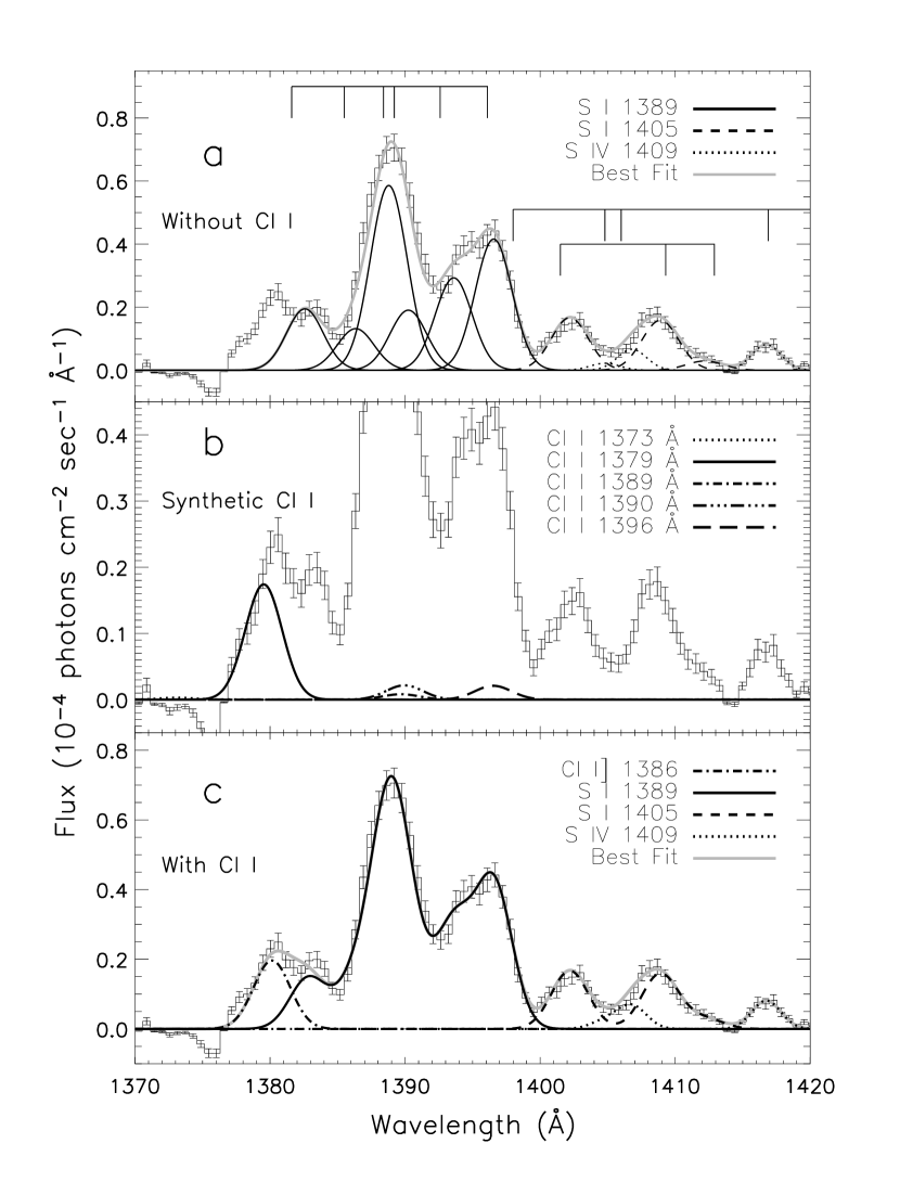
Figure 4: Flux spectrum of the GHRS data previously shown in Figure 2, limited to the range 1370–1420 Å. (a) Gaussian fits to S I $\lambda$1389 (solid), S I $\lambda$1405 (dashed), and S IV] $\lambda$1406 (dotted). Best total fit is in gray. Excess flux shortward of the S I $\lambda$1389 multiplet is seen at a SNR of $\sim\mskip 3.0mu$10. (b) Synthetic spectrum of the Cl I] $\lambda$1386 multiplet assuming optically thin line ratios. (c) Same as (a) with the Gaussian fit to the detected 1379.5 Å  transition of Cl I] $\lambda$1386 (dash-dotted). The solid gray line is the total fit for the region.

The S I $\lambda$1389 and S I $\lambda$1405 spectral fits are shown in Figure 4a. There are six components in the S I $\lambda$1389 multiplet and three components in the S I $\lambda$1405 multiplet (Table 2). Atomic data for the UV sulfur transitions are limited, especially for the S I $\lambda$1389 multiplet which has only two published oscillator strength values for the individual transitions, one theoretical (Varsavsky, 1961) and one experimental (Müller, 1968), differing by several orders of magnitude. The 3s 3p^5 3P°  state of this multiplet is highly mixed, difficult to correctly represent in theoretical calculations, and in Io’s environment is excited by low-temperature, near-threshold electrons. Because of this, neither the experimental nor the theoretical data are ideal. Although both give similar line ratios, Morton (2003) reports the experimental data (Müller, 1968) which we also utilize. Our observed relative strengths significantly disagree with the expected optically thin values. Specifically, transitions with an upper level of $J$=2, 1388 Å  and 1396 Å, are 2–3 times larger than expected. However, our values are reasonably consistent with those observed by Retherford (2002). What looks to be a large discrepancy between the two data sets in the relative strengths of the 1388/1389 lines is a result of blending of these two transitions. If analyzed as a pair rather than individual lines, comparable values of $\sim\mskip 3.0mu$5 $\pm$ 2 for (1388+1389)/1381 emerge. We do not attribute the disagreement between observed data from Io and published atomic data for S I $\lambda$1389 to optical depth effects since the multiplet oscillator strength is 2–3 orders of magnitude smaller than those of other allowed sulfur multiplets and is comparable in magnitude to the forbidden lines, which do not experience self-absorption. In addition, we find that the strongest lines in the data, which are expected to be strongest in the optically thin case and hence would be most affected by optical depth, are the transitions for which the ratios are inconsistently large, in the opposite sense of optical thickness effects.

The relative strengths of the S I $\lambda$1405 multiplet also differ from the expected optically thin values, which we attribute to optical thickness effects and spectral contamination by the Io plasma torus. The weakest line, 1413 Å, is marginally detected while the remaining lines, 1401 Å  and 1409 Å, are comparable in strength, corresponding to the redistribution of line flux from the strongest line, 1401 Å, to the longer wavelength line, 1409 Å. The oscillator strength, optical thickness effects, and configuration of this multiplet resemble that of the S I $\lambda$1814 allowed multiplet in Io’s atmosphere which has also been interpreted to be optically thick (Feaga, McGrath, & Feldman 2002; McGrath et al. 2000; Ballester et al. 1987). The ratio of 1409 Å  to 1413 Å, however, is much higher than expected even in the optically thick case where 1409 Å  is preferentially pumped by 1401 Å  and is the result of S IV torus emission blending with the S I $\lambda$1405 multiplet, as explained below.

We investigate a feature longward of the S I $\lambda$1405 multiplet, marked with a Y in Figure 2, which is detected at a SNR of 5 and is coincident in wavelength with a S IV transition at 1416.9 Å  to determine if the S IV multiplet, composed of 5 transitions from 1398–1424 Å, contributes to the inconsistent line ratios discussed above for the S I $\lambda$1405 multiplet. Using the spectral fitting routine, and allowing the FWHM of the S IV multiplet to differ from the emissions from Io, the weak 1398 Å  line is not detected. The 1424 Å  line is coincident with a much stronger S I $\lambda$1429 multiplet and we do not attempt to disentangle its expected minimal contribution. Fits to the remaining two lines, 1404 Å  and 1406 Å, provide a better overall fit to the data, although the error bars on the 1404 Å  line are large and contribute to the uncertainty of the S I $\lambda$1405 fluxes. The 1406 Å  and 1417 Å  lines are expected to be the strongest lines of S IV] $\lambda$1406 (Figure 4a). As detected, they have relative line strengths consistent with those found using atomic data from Tayal (1999, 2000) and observed in the Io torus (Moos & Clarke, 1981; Moos et al., 1991). We tentatively identify these emissions as S IV originating from the Io plasma torus since the GHRS field of view is larger than the disk of Io and the line of sight from HST to Io intersects the torus.

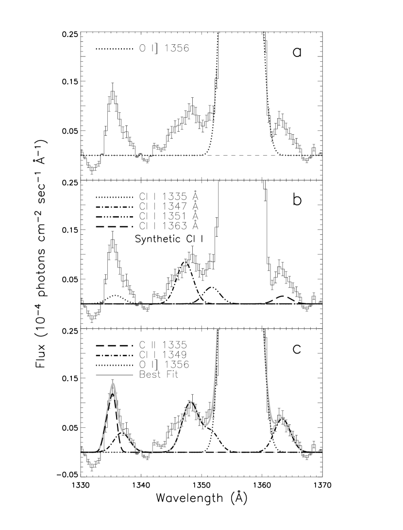
Figure 5: (a) Gaussian fit to the O I] $\lambda$1356 doublet (dotted) previously shown in Figure 3 with excess flux flanking the oxygen emission above the noise level. (b) Synthetic spectrum of the Cl I $\lambda$1349 multiplet emission assuming optically thin line ratios. (c) Gaussian fits to the detected Cl I $\lambda$1349 transitions (dash-dotted) are added to the oxygen doublet (dotted). The chlorine transition at 1335 Å  is contaminated by a reflected solar component, C II $\lambda$1335, whose fit is shown with a dashed line. In our best fits, the carbon is assumed to account for most of the flux at 1335 Å  based on the FWHM and amplitude analysis of the line. See text for discussion. The total fit is in gray.

Additional emission, not associated with the oxygen and sulfur features, is obvious in Figures 4 and 5 flanking the O I] $\lambda$1356 doublet and the S I $\lambda$1389 multiplets. Emission near 1335 Å  and 1379 Å  is seen in spectra from all 8 dates of observation (Figure 1). In the co-added flux spectrum, the 1379 Å  emission is detected at a SNR of 10 (Figure 4). The emission features at 1335 Å, 1347 Å, and 1363 Å  (Figure 5) are detected at a SNR of $\sim\mskip 3.0mu$6.

Two multiplets of chlorine occur in the 1330–1400 Å region, a dipole allowed transition, Cl I $\lambda$1349, consisting of four lines and Cl I] $\lambda$1386, a forbidden transition consisting of five lines (Table 2). Synthetic profiles of these multiplets using optically thin line ratios are shown in Figures 4b and 5b. Using the same $\chi^{2}$ minimization method described above in which the amplitude is a free parameter, wavelength is constrained, and FWHM is fixed, fits are made to these previously unidentified features and are presented in Figure 4c and 5c. Using data acquired by STIS with higher spectral resolution but lower SNR, Retherford (2002) presents the detection of one chlorine line per multiplet, 1347.2 Å  and 1379.5 Å.

In the Cl I] $\lambda$1386 multiplet, lines other than 1379.5 Å, which is the strongest line of the multiplet accounting for more than 75% of the multiplet’s total strength, are either too weak or blended with the sulfur to unambiguously identify. The component at 1373.1 Å  is not detected, consistent with its very small strength compared to the 1379.5 Å  line. We neglect all but the 1379.5 Å  line in the subsequent flux analysis.

The flux ratio of 1347.2 Å  to 1363.5 Å  in the Cl I $\lambda$1349 multiplet is almost a factor of 4 lower than expected in the optically thin case, indicating the redistribution of flux between the two lines. Because of this, we infer that the multiplet is optically thick. The flux ratio of 1335.7/1351.7 is 2.6, more than a factor of 5 higher than the expected optically thin value for the two Cl I $\lambda$1349 lines at these wavelengths. As discussed further below, we attribute the majority of the integrated flux for the 1335 Å  feature to a factor other than optical depth effects.

The 1335.7 Å  feature of the Cl I $\lambda$1349 multiplet is not well fit with one Gaussian of 3.2 Å  FWHM. The best fit for a single Gaussian at 1335.7 Å  results in a line with a FWHM of 1.8 Å. Considering the unusually high flux and the smaller FWHM of the 1335.7 Å  feature, we attribute the majority of the integrated flux at 1335.7 Å  not to chlorine but to the strong C II $\lambda$1335 emission multiplet, with a component at 1335.7 Å, in the solar spectrum reflected from Io and detected previously from both Europa and Ganymede (Hall et al., 1995, 1998). We model the reflection of the C II $\lambda$1335 multiplet from Io’s disk and determine that C II has a smaller FWHM than Iogenic emissions for which the FWHM are broadened by the geometry of the equatorial spots and limb glow morphology. To correctly account for the solar carbon and Iogenic chlorine contribution to 1335 Å, we re-fit the feature with three Gaussians, two representing the 1334.5 Å  and 1335.7 Å  lines of C II with FWHM of 1.4 Å  and one chlorine line with a FWHM of 3.2 Å  (Figure 5c). These fluxes are listed in Table 2.

This is the first reported detection of C II $\lambda$1335 from Io, providing a unique measurement of the UV geometric albedo of the satellite at this wavelength. Following Feldman et al. (2000), Io’s albedo is calculated using a weighted average of solar spectra from the UARS SOLSTICE experiment (Woods et al., 1996) acquired on the dates of HST/GHRS Io observation. All observations occurred during periods of minimal solar activity. With no SO₂ absorption, the best fit to the data in Figure 5c gives a disk averaged geometric albedo of 0.83$\pm$0.35%. However, the albedo calculation at 1335 Å  is sensitive to the SO₂ column density. An SO₂ column density of $\sim\mskip 3.0mu$10¹⁶ cm^-2 would increase the derived albedo to 1.0%. Feldman et al. (2000) estimate albedos of 1.5% for HST/STIS data acquired in 1997 and 1.9% for 1998 by fitting the continuum between 1520 Å and 1700 Å. In this wavelength interval, the albedo calculation is much less sensitive to the SO₂ column since the absorption cross section of SO₂ is half that at 1335 Å. Including a latitudinally varying surface albedo and a modeled SO₂ column density, which when disk averaged is $\sim\mskip 3.0mu$1$\times$10¹⁶ cm^-2, Strobel & Wolven (2001) derive albedos ranging from 2.2–3.1% to match the mid-latitude Lyman-$\alpha$ measurements in the 1998 HST/STIS data. An SO₂ column density of 3.6–8.0$\times$10¹⁶ cm^-2 would easily bring our albedo value into agreement with those of Feldman et al. (2000) and Strobel & Wolven (2001) which is consistent with the known properties of Io’s SO₂ atmosphere (McGrath et al., 2004). Differing values of the geometric albedo estimated by Feldman et al. (2000) and Strobel & Wolven (2001) for the same data using similar SO₂ column densities may suggest a wavelength dependence of the UV albedo rather than measurable variations in the SO₂ atmosphere.

We have also considered the contribution of solar resonant scattering to the Cl I $\lambda$1349 multiplet. As stated previously, Cl I 1335.7 Å  is coincident in wavelength with a strong solar C II transition. Since the Cl I 1335.7 Å  and 1351.7 Å  lines share the same upper level, it is possible for 1351.7 Å  to be pumped by the strong solar carbon line at 1335.7 Å. Including a curve of growth to account for self-absorption in our data where the Cl I $\lambda$1349 multiplet is optically thick, the fluorescence saturates at 0.02$\mskip 3.0mu\times$ 10${}^{-4}\mskip 3.0mu$photons cm${}^{-2}\mskip 3.0mu$s^-1. We conclude that the induced fluorescence of 1351.7 Å  is negligible.

3 ANALYSIS

Since our data set lacks spatial information, we rely on Retherford (2002) for information about the spatial distribution of the chlorine emission at Io. He finds that the emitting chlorine has similar morphology to that of atomic oxygen and sulfur, and is therefore assumed to be located at higher altitudes than the bulk of the SO₂ and to be excited by the same electron impact mechanism as oxygen and sulfur. This assumption allows us to give concurrent estimates of the relative abundances of these species from the same spectrum. For a transition excited by electron impact, the total measured brightness for a multiplet along the line of sight ($B_{ij}$) is related to the density of the emitting species ($n_{s}$), the electron density ($n_{e}$), and the temperature-dependent electron excitation rate coefficient ($Q_{ij}$) of the multiplet:

$${B_{ij}(T_{e})}=\int{n_{s}n_{e}Q_{ij}(T_{e})dl}.$$

In calculating ratios of species detected along the same line of sight, the dependence on the electron density and line of sight conditions is removed and an approximate proportionality is established as a function of electron temperature ($T_{e}$). Since the electron impact excitation rate coefficient is a function of electron temperature, we choose a nominal value 5 eV for $T_{e}$. Incorporating the Cl I $\lambda$1349 and O I] $\lambda$1356 cross sections from Ganas (1988) and D. F. Strobel (2002, private communication), respectively, Retherford (2002) made detailed calculations of the rate coefficients which are adopted here (Table 3). Using recently published atomic data (Zatsarinny & Tayal, 2002), the electron impact excitation rates for several sulfur multiplets are calculated and listed in Table 3. A liberal error estimate of 30% for the rate coefficients is propagated through the relative abundance calculations.

To achieve the best estimate of the Cl/O, Cl/S, and S/O abundance ratios, total measured fluxes of Cl I $\lambda$1349, O I] $\lambda$1356, S I $\lambda$1429, and S I $\lambda$1479 are selected for the calculation. Cl I $\lambda$1349 is chosen since it is the least blended chlorine multiplet and the only chorine multiplet in our data for which reliable atomic data have been published. Two allowed sulfur multiplets are selected in lieu of forbidden sulfur multiplets and the contaminated S I $\lambda$1405 multiplet. S I $\lambda$1429 and S I $\lambda$1479 are dominant sulfur transitions in the spectral range of the data with high SNR and better atomic data than the other sulfur multiplets. Following Feaga et al. (2002), we assume a 40% : 60% contribution to the total 1479 Å  flux of the individual forbidden and allowed multiplets, respectively, as they are not resolved in the GHRS data. With these fluxes and the corresponding electron rate coefficients from Table 3, we estimate and present in Table 4 disk averaged abundance ratios. Because of the large errors for the abundance ratios due in part to the uncertainty in the electron impact rate coefficients, the results are insensitive to $T_{e}$ for a range of 3–7 eV.

To quantify the contribution of the equatorial spot emission to the total emission from Io, we present the STIS equatorial spot to GHRS disk averaged emission flux ratio for Cl I $\lambda$1349 and compare it to the spot to disk ratio of O I] $\lambda$1356 in STIS data alone. The equatorial spot flux listed in Table 2 is the average flux for a single spot extracted using a 0.049 (arcsec)² solid angle (Retherford, 2002) and the disk flux is calculated from the emission contained in the 1.74^′′ square GHRS aperture. The equatorial spots are 2–5% of the total disk emission for chlorine. For comparison, an oxygen spot to disk ratio of 2–5% is estimated using the data from Retherford (2002). The chlorine and oxygen spot to disk values are similar.

4 DISCUSSION

Utilizing the definition of optical depth, $\tau\mskip 3.0mu=\mskip 3.0mu{\cal N}\sigma$, where ${\cal N}$ is the column density and $\sigma$ is the absorption cross section, and the determination of the Cl I $\lambda$1349 multiplet being optically thick in our data ($\tau>\mskip 3.0mu$1), a lower bound to the disk averaged chlorine column density of 2.3$\times$10¹² cm^-2 is implied. The chlorine absorption cross section is calculated with the oscillator strength from Biémont, Gebarowski, & Zeippen (1994) at a temperature of 1000 K. In the same manner, the S I $\lambda$1405 multiplet appears to be optically thick in our data giving a lower bound to the disk averaged sulfur column density of 2.4$\times$10¹³ cm^-2 using an oscillator strength from Tayal (1998). This result is consistent with the disk averaged sulfur column density lower bound estimated by Feaga et al. (2002) for the S I $\lambda$1814 multiplet in IUE and FOS data. This independent estimate of the sulfur column density lends credence to the range of sulfur column densities found by Feaga et al. (2002).

The S/O results presented here are in agreement with the Wolven et al. (2001) analysis of HST/STIS data. They find a disk averaged S/O brightness ratio of 1 : 0.81 when comparing the combined S I $\lambda$1479 multiplets to the O I] $\lambda$1356 doublet. Applying the 40% : 60% contribution of the forbidden and allowed multiplets (Feaga et al., 2002), respectively, to the Wolven et al. (2001) analysis and utilizing the rate coefficients from Table 3, their brightness ratio translates to an S/O abundance ratio of 0.10 $\pm$ 0.06.

Combining the S/SO₂ ratio of 3–7$\times$10^-3 measured at three spatially resolved locations by McGrath et al. (2000) with our results, an estimate of the Cl/SO₂ ratio can be made, which leads to an approximate Cl/SO₂ abundance ratio of 3.0–7.0$\times$10^-4 (Table 4). In addition, combining the O/SO₂ ratio of 0.05 inferred with Cassini data (Geissler et al., 2004) with our results gives a Cl/SO₂ value of 8.5$\times$10^-4. Recently, Lellouch et al. (2003) detected a comparable abundance of NaCl with a disk averaged NaCl/SO₂ ratio of 7$\times$10^-4–0.02 if NaCl is more localized than SO₂, with a preferred value of 3.5$\times$10^-3 (Table 4).

In assessing escape rates of sodium, chlorine, and NaCl from Io, Moses et al. (2002b) establish that chlorine and sodium have escape fluxes 10–20 times larger than NaCl. Our estimated atmospheric chlorine abundance and the NaCl abundance of Lellouch et al. (2003) are both 1–2 orders of magnitude lower than the 1% torus chlorine mixing ratio (Feldman et al., 2001) indicating that there exists an intricate relationship between the transport of volcanic gases to the upper atmosphere and escape to the torus. There may also be a higher concentration of chlorine compared to sulfur and oxygen near volcanic outflows which are at lower altitudes than we probe and would boost the overall atmospheric chlorine abundance measured in our data. In the Pele-type volcanic atmospheres modeled by Moses et al. (2002b) which include chlorine, sodium, and potassium, the initial chlorine abundance is assumed from the high chlorine torus abundance of Schneider et al. (2000). They do not check the sensitivity of their models to lower chlorine abundances, so we do not compare our results for chlorine. We do however compare the S/O abundance ratios. Moses et al. (2002a) determine an equilibrium ratio of 10 for S/O, $\sim\mskip 3.0mu$50 times larger than our data shows. This suggests that either the initial oxygen abundances in the models are too low or the disk averaged atmosphere we detect at Io is dominated by Prometheus-type (SO₂ dominated) outflows rather than Pele-type (sulfur dominated). Moses et al. (2002a) do not check the sensitivity of their models to the initial S/O abundance.

Lastly, our Cl/S ratio adds plausibility to the identification of solid Cl₂SO₂ or ClSO₂ in NIMS/Galileo spectra near the volcanic center of Marduk as suggested by Schmitt & Rodriguez (2003). Unidentified absorption features are present in the infrared spectra and based on their spectroscopic arguments, Cl₂SO₂ is the favorite candidate with ClSO₂ a potential alternative. Schmitt & Rodriguez (2003) estimate that for abundant Cl₂SO₂ formation, the gaseous [Cl-(Na+K)]/S ratio in a volcanic plume needs to be larger than 0.015, and for ClSO₂, the ratio must be even larger. When there is an excess of halogens as compared to alkalis, Cl/(Na+K) $>$ 1, sulfur chlorides and oxychlorides are formed with the surplus chlorine. Since volcanic outgassing is assumed to be the only source of chlorine in Io’s atmosphere, plumes should have at least a comparable, most likely higher, abundance of chlorine relative to the disk averaged atmosphere. For comparable Cl and NaCl disk averaged abundances, consistent with our data and that of Lellouch et al. (2003), an estimated Cl/Na ratio of $\sim\mskip 3.0mu$10 is shown in Figure 3d of Fegley & Zolotov (2000), and for our Cl/S ratio of 0.1, a Cl/Na ratio $\geq\mskip 3.0mu$2 can be estimated from Figure 5 of Fegley & Zolotov (2000). These ratios imply that gaseous chlorine is at least twice as high in abundance as sodium. Therefore, our disk averaged Cl/S ratio is consistent with the requirements of Schmitt & Rodriguez (2003) for the presence of Cl₂SO₂ or ClSO₂.

Table 1: Table of Observations

Obs Name	Date	Time	Exposure	Io OLG	Io SYS III
		UT	(s)	($\arcdeg$)	($\arcdeg$)
z2eh0506	1994 Jun 06	16:48:41	620.0	98	140
z2eh0508	1994 Jun 06	18:06:11	1580.0	109	176
z2eh0306	1994 Jun 14	15:57:23	1580.0	279	52
z2eh0308	1994 Jun 14	17:34:05	620.0	293	97
z2eh0306	1994 Jun 16	09:48:23	1580.0	274	135
z2eh0408	1994 Jun 16	11:24:37	600.0	287	176
z2gd0e02	1994 Jul 15	05:24:16	1555.5	17	276
z2v9a102	1995 Sep 21	20:03:23	972.8	18	73
z2v9a104	1995 Sep 21	20:26:59	942.4	21	84
z2v9a106	1995 Sep 21	21:33:59	972.8	30	116
z2v9a108	1995 Sep 21	21:58:23	790.4	34	126
z2v90308	1996 Mar 23	19:20:52	972.8	338	31
z2v9030a	1996 Mar 23	19:44:34	942.4	341	43
z2v9020a	1996 Jun 26	04:26:53	851.2	106	350
z2v9020e	1996 Jun 26	06:03:22	851.2	119	35
z2v9020h	1996 Jun 26	07:21:40	699.2	130	72
z2v9020i	1996 Jun 26	07:35:53	364.8	132	77
z2v9020k	1996 Jun 26	08:49:34	760.0	143	112
z2v9020m	1996 Jun 26	09:10:10	790.4	146	121
z2v9020o	1996 Jun 26	10:26:10	851.2	156	156
z2v9020q	1996 Jun 26	10:48:22	851.2	160	167
z3eta102	1996 Sep 04	11:09:10	972.8	12	67
z3eta104	1996 Sep 04	11:32:59	1033.6	16	79
z3eta106	1996 Sep 04	12:45:10	668.8	26	112
z3eta109	1996 Sep 04	13:13:16	832.0	30	125

Table 2: Atomic Transitions and Measured Fluxes

Species	Configuration	$J_{u}$	$J_{l}$	$\lambda_{lab}$	$\lambda_{fit}$	Relative	GHRS Flux	STIS Flux
				(Å)	(Å)	strength	(10${}^{-4}\mskip 3.0mu$photons  cm${}^{-2}\mskip 3.0mu$s-1)
C II	2s 2p2 2D$\mskip 3.0mu\to$ 2s2 (1S) 2p 2P°	3/2	1/2	1334.53	1334.30	5.0	0.08 $\pm$ 0.07
		3/2	3/2	1335.66		1.0
		5/2	3/2	1335.71	1335.40	9.0	0.16 $\pm$ 0.07
Cl I	3s2 3p4 (3P) 4s 2P$\mskip 3.0mu\to$ 3s2 3p5 2P°	1/2	3/2	1335.73	1336.80	1.1	0.13 $\pm$ 0.06
		3/2	3/2	1347.24	1348.13	5.5	0.34 $\pm$ 0.08	0.012 $\pm$ 0.003
		1/2	1/2	1351.66	1351.52	2.2	0.14 $\pm$ 0.08	0.006 $\pm$ 0.004
		3/2	1/2	1363.45	1363.35	1.0	0.23 $\pm$ 0.04
O I	2s2 2p3 3s 5S°$\to$ 2s2 2p${}^{4}\mskip 3.0mu{}^{3}$P	2	2	1355.60	1355.56	3.1	7.71 $\pm$ 0.34	0.830 $\pm$ 0.020
		2	1	1358.51	1358.34	1.0	2.31 $\pm$ 0.28	0.230 $\pm$ 0.010
Cl I	3s2 3p4 (3P) 4s 4P$\mskip 3.0mu\to$ 3s2 3p${}^{5}\mskip 3.0mu{}^{2}$P°	1/2	3/2	1373.12		1.0
		3/2	3/2	1379.53	1380.14	58.8	0.67 $\pm$ 0.22	0.036 $\pm$ 0.006
		5/2	3/2	1389.69		2.8
		1/2	1/2	1389.96		7.3
		3/2	1/2	1396.53		7.1
S I	3s 3p5 3P°$\to$ 3s2 3p${}^{4}\mskip 3.0mu{}^{3}$P	1	2	1381.55	1382.83	1.0	0.50 $\pm$ 0.16	0.042 $\pm$ 0.006
		0	1	1385.51	1386.34	0.8	0.45 $\pm$ 0.10	0.046 $\pm$ 0.006
		2	2	1388.44	1388.79	1.7	2.00 $\pm$ 0.35	0.130 $\pm$ 0.007
		1	1	1389.15	1390.24	0.3	0.65 $\pm$ 0.19	0.086 $\pm$ 0.006
		1	0	1392.59	1393.60	1.0	1.00 $\pm$ 0.22	0.051 $\pm$ 0.006
		2	1	1396.11	1396.56	1.8	1.42 $\pm$ 0.23	0.127 $\pm$ 0.008
S IV	3s 3p2 4P°$\to$ 3s2 3p 2P°	3/2	1/2	1398.04		0.2
		1/2	1/2	1404.81	1404.80	1.0	0.06 $\pm$ 0.18
		5/2	3/2	1406.02	1406.80	3.5	0.18 $\pm$ 0.10
		3/2	3/2	1416.89	1416.75	3.0	0.22 $\pm$ 0.01
		1/2	3/2	1423.84		0.8
S I	3s2 3p3 5s 3S°$\to$ 3s2 3p${}^{4}\mskip 3.0mu{}^{3}$P	1	2	1401.51	1402.20	5.3	0.57 $\pm$ 0.16
		1	1	1409.34	1408.90	3.1	0.54 $\pm$ 0.08
		1	0	1412.87	1412.20	1.0	0.10 $\pm$ 0.08
S I	3s2 3p3 3d 3D°$\to$ 3s2 3p${}^{4}\mskip 3.0mu{}^{3}$P			1429.11			5.78 $\pm$ 0.22
S I	3s2 3p3 3d 5D°$\to$ 3s2 3p${}^{4}\mskip 3.0mu{}^{3}$P			1477.31			6.69 $\pm$ 0.27
S I	3s2 3p3 4s${}^{\prime}\mskip 3.0mu{}^{3}$D°$\to$ 3s2 3p${}^{4}\mskip 3.0mu{}^{3}$P			1478.50			10.03 $\pm$ 0.40

Table 3: Electron Impact Excitation Rate Coefficients

Species	Rate Coefficient
	(cm3 s-1)
Cl I $\lambda$1349	1.6$\times$10-9
O I] $\lambda$1356	3.2$\times$10-10
S I $\lambda$1429	1.1$\times$10-9
S I $\lambda$1479	1.8$\times$10-9

Table 4: Abundance Ratios at Io

Species	Relative Atmospheric	Reference
	Abundance
Cl/O	0.017 $\pm$ 0.008	1
Cl/S	0.10 $\pm$ 0.05	1
S/O	0.18 $\pm$ 0.08	1
NaCl/SO2	7$\times$10-4–0.02	2
S/SO2	(3–7)$\times$10-3	3
O/SO2	0.05	4
Cl/SO2	(3.0–8.5)$\times$10-4	1,3,4

References. — (1) This paper; (2) Lellouch et al. 2003; (3) McGrath et al. 2000; (4) Geissler et al. 2004.

Figure 1: Individual flux spectra of Io’s atmospheric emissions in the wavelength range 1330–1410 Å  taken with HST/GHRS from 1994–1996 to illustrate the variation from date to date and the need for co-adding the data to achieve better signal to noise. All data are on the same scale with the zero flux line shifted for display purposes. The X’s indicate possible chlorine emission.

Figure 2: Co-added flux spectrum of Io’s atmospheric emissions in the wavelength range 1230–1510 Å  taken with HST/GHRS from 1994–1996. Several sulfur and oxygen features previously identified in Io’s atmosphere are indicated. The X’s indicate possible chlorine emission. Y indicates possible S IV. The portion of the spectrum in boldface is analyzed in this paper.

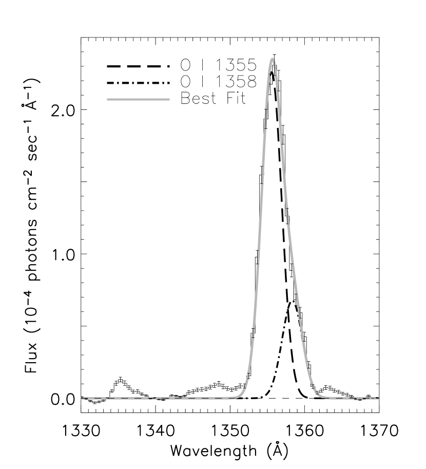
Figure 3: Gaussian fits to the O I] $\lambda$1356 emission in the flux spectrum of the co-added GHRS data previously shown in Figure 2. The 1355.6 Å  (dashed) and 1358.5 Å  (dash-dotted) fits are shown separately and the total fit is in gray.

References

- Ballester et al. (1987) Ballester, G. E., et al. 1987, ApJ, 319, L33
- Ballester et al. (1996) Ballester, G. E., et al. 1996, BAAS, 28, 1156
- Ballester et al. (1997) Ballester, G. E., et al. 1997, BAAS, 29, 980
- Biémont, Gebarowski, & Zeippen (1994) Biémont, E., Gebarowski, R., & Zeippen, C. J. 1994, A&A, 287, 290
- Durrance et al. (1995) Durrance, S. T., Feldman, P. D., Blair, W. P., Davidsen, A. F., Kriss, G. A., Kruk, J. W., Long, K. S., & Moos, H. W. 1995, ApJ, 447, 408
- Feaga et al. (2002) Feaga, L. M., McGrath, M. A., & Feldman, P. D. 2002, ApJ, 570, 439
- Fegley & Zolotov (2000) Fegley, B., Jr., & Zolotov, M. Y. 2000, Icarus, 148, 193
- Feldman et al. (2001) Feldman, P. D., Ake, T. B., Berman, A. F., Moos, H. W., Sahnow, D. J., Strobel, D. F., Weaver, H. A., & Young, P. R. 2001, ApJ, 554, L123
- Feldman et al. (2000) Feldman, P. D., et al. 2000, Geophys. Res. Lett., 27, 1787
- Feldman et al. (2004) Feldman, P. D., Strobel, D. F., Moos, H. W., & Weaver, H. A. 2004, ApJ, 601, 583
- Ganas (1988) Ganas, P. S. 1988, J. Appl. Phys., 63, 277
- Geissler et al. (2004) Geissler, P., McEwen, A., Porco, C., Strobel, D., Saur, S., Ajello, J., & West, R. 2004, Icarus, submitted
- Hall et al. (1994) Hall, D. T., et al. 1994, ApJ, 426, L51
- Hall et al. (1998) Hall, D. T., Feldman, P. D., McGrath, M. A., & Strobel, D. F. 1998, ApJ, 499, 475
- Hall et al. (1995) Hall, D. T., Strobel, D. F., Feldman, P. D., McGrath, M. A., & Weaver, H. A. 1995, Nature, 373, 677
- Jessup et al. (2004) Jessup, K. L., Spencer, J. R., Ballester, G. E., Howell, R., Roesler, F., Vigil, M., & Yelle, R. 2004, Icarus, in press
- Kriss (1994) Kriss, G. 1994, in ASP Conf. Ser. 61, Astronomical Data Analysis Software and Systems III, ed. D. R. Crabtree, R. J. Hanisch, & J. Barnes (San Francisco: ASP), 437