X-ray flares from the ultra-luminous X-ray source in NGC 5408

We have studied an ultra-luminous X-ray source (ULX) in the dwarf galaxy NGC 5408 with a series of XMM-Newton observations, between 2001 July and 2003 January. We find that its X-ray spectrum is best fitted with a power law of photon index $\Gamma\approx 2.6$–$2.9$ and a thermal component with blackbody temperature $kT_{\rm bb}\approx 0.12$–$0.14$ keV. These spectral features, and the inferred luminosity $\approx 10^{40}$ erg s^-1 in the $0.3$–$12$ keV band, are typical of bright ULXs in nearby dwarf galaxies. The blackbody plus power-law model is a significantly better fit than either a simple power law or a broken power law (although the latter model is also acceptable at some epochs). Doppler-boosted emission from a relativistic jet is not required, although we cannot rule out this scenario. Our preliminary timing analysis shows flaring behaviour which we interpret as variability in the power-law component, on timescales of $\sim 10^{2}$ s. The hard component is suppressed during the dips, while the soft thermal component is consistent with being constant. The power density spectrum is flat at low frequencies, has a break at $\nu_{\rm b}\approx 2.5$ mHz, and has a slope $\approx-1$ at higher frequencies. A comparison with the power spectra of Cyg X-1 and of a sample of other BH candidates and AGN suggests a mass of $\sim 10^{2}M_{\odot}$. It is also possible that the BH is at the upper end of the stellar-mass class ($M\sim 50M_{\odot}$), in a phase of moderately super-Eddington accretion. The formation of such a massive BH via normal stellar evolution may have been favoured by the very metal-poor environment of NGC 5408.

1 Introduction

Ultra-luminous X-ray sources (ULXs) are point-like sources, not including galactic nuclei and young supernova remnants, with apparent luminositites higher than the Eddington limit for a stellar-mass accreting black hole (BH), ie, with $L_{X}\ga 3\times 10^{39}$ erg s^-1 (Fabbiano 1992; Colbert & Mushotzky 1999; Roberts & Warwick 2000). The true nature of these objects is still open to debate. The fundamental issue is whether the emission is isotropic or beamed along our line-of-sight; in the latter case, the total luminosity would of course be lower than the isotropic value. A possible scenario for geometrical beaming is a super-Eddington mass inflow during phases of thermal-timescale mass transfer (King 2002). Relativistic beaming, associated with Doppler boosting, would instead be the effect of our looking into the jet of a microquasar (Körding et al. 2002). Alternatively, if the emission is isotropic and the Eddington limit is not violated, ULXs must be fuelled by accretion onto intermediate-mass BHs, with masses $\sim 10^{2}\,M_{\odot}$. Possible mechanisms of formation of such massive remnants include the collapse of massive population III stars (Madau & Rees 2001), or runaway stellar mergers in young clusters (Portegies Zwart et al. 2004).

A ULX in the starburst dwarf irregular galaxy NGC 5408 could help discriminate between these two alternatives. Radio observations of this galaxy (Stevens et al. 2002) showed four main emission regions, mostly coincident with massive young star clusters and H$\alpha$ emission. The X-ray emission is dominated by a single point source, with a luminosity $>10^{40}$ erg s^-1 (Fabian & Ward 1993; Kaaret et al. 2003), located outside the HII regions, but apparently coincident with a weak, steep-spectrum radio source. On the basis of the X-ray, radio, and optical fluxes, Kaaret et al. (2003) concluded that the most likely explanation for the ULX was beamed relativistic jet emission from a stellar-mass BH. However, they could not rule out an intermediate-mass BH model. In this paper we present the first results of our XMM-Newton study of the ULX in NGC 5408, providing new insights into the nature of this source.

2 Observations and data analysis

NGC 5408 was observed with the European Photon Imaging Camera (EPIC) and the Reflection Grating Spectrometer (RGS) on board XMM-Newton in 2001 July–August, 2002 July and 2003 January (Table 1). The Optical Monitor was blocked because of a bright foreground star in the field. In this paper, we present preliminary results from the EPIC data; more detailed results are left to further work.

The thin-filter, full-frame mode was used for the MOS and pn cameras. We processed the Observation Data Files with standard tasks in Version 5.4 of the Science Analysis System (SAS). After inspecting the background flux of each exposure, we rejected various intervals with background flares in Rev. 301 and Rev. 574. A high, flaring background affected the whole exposures in Rev. 483: the average background count rate was $\approx 20\%$ of the ULX count rate in the source extraction region. We retained that exposure (the only one available for 2002), with the caveat that the timing analyses may be affected by larger errors. For all other exposures, the background rate in the selected good-time-intervals is typically $\sim 1$–$2\%$ of the source count rate. Technical problems during Rev. 313 meant that the pn was not activated, while the usable part of the MOS exposures lasted only 6.9 ks despite a nominal exposure time of 7.5 ks. We filtered the event files, selecting only the best-calibrated events (pattern $\leq 12$ for the MOSs, pattern $\leq 4$ for the pn), and rejecting flagged events. We also checked that the source was not piled-up, with the SAS task epatplot.

For each exposure, we used a 30″-radius source extraction region, with the background extracted from other regions in the same CCD. We built appropriate response functions with the SAS tasks rmfgen and arfgen. We fitted the background-subtracted spectra with standard models in XSPEC v.11.3 (Arnaud 1996); owing to the uncertainties in the EPIC responses at low energies, we used only the $0.3$–$12$ keV range. Firstly, we analysed the individual pn and MOS spectra from each observation. After ascertaining that they were consistent with each other, we coadded them with the method described in Page et al. (2003), to increase the signal-to-noise ratio. Thus, we obtained one combined EPIC spectrum of the ULX from each epoch. With the same method, we also built an average EPIC spectrum of all the observations from 2001. For the timing analysis presented here, we selected all the good-time-intervals when both the MOS and pn were operating (except for the lightcurve in Rev. 313, for which only the MOS is available), and we retained the events in the $0.2$–$12$ keV range. We used standard tasks in FTOOLS (Blackburn 1995) to obtain background-subtracted lightcurves and power-density spectra.

Table 1: XMM-Newton/EPIC observation log for NGC 5408.

Date	Obs ID	Start time	Stop time	GTI
2001 Jul 31	0112290501	pn: 12:49:45	14:13:05	3.8 ks
	(Rev. 301)	MOS: 12:12:08	14:17:21	4.1 ks
2001 Aug 08	0112290601	pn: 10:22:14	11:45:34	4.5 ks
	(Rev. 305)	MOS: 09:43:01	11:48:13	7.4 ks
2001 Aug 24	0112290701	pn: -	-	-
	(Rev. 313)	MOS: 21:58:47	00:05:39	6.9 ks
2002 Jul 29	0112291001	pn: 08:23:12	10:08:22	4.9 ks
	(Rev. 483)	MOS: 08:01:02	10:11:28	7.7 ks
2003 Jan 28	0112291201	pn: 00:06:06	01:29:57	3.0 ks
	(Rev. 574)	MOS: 23:43:56	01:18:14	3.3 ks

3 Main results

3.1 Spectral analysis

Based on a short (4.7 ks) Chandra observation, it was suggested (Kaaret et al. 2003) that the X-ray spectrum of this ULX could be fitted equally well by a broken power law (break energy $\approx 0.65$ keV), or by an absorbed blackbody plus power-law model ($kT_{\rm bb}\approx 0.11$ keV; photon index $\Gamma\approx 2.8$). The broken power-law model would support the interpretation of this source as beamed emission via inverse-Compton scattering of optical/UV photons by a relativistic jet (Georganopoulos et al. 2001; Kaaret et al. 2003).

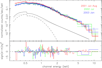
Figure 1: Coadded EPIC spectra of the ULX in 2001 Jul–Aug (blue, with its best-fit blackbody plus powerlaw model), 2002 July (red), 2003 Jan (green). Also overplotted: the best-fit model for the 2001 spectrum, in photons cm^-1 s^-1 keV^-1 (arbitrarily shifted for clarity).

In our XMM-Newton study, we confirm that a simple absorbed power-law model is ruled out ($\chi^{2}_{\nu}\ga 1.4$ for all spectra). We then consider a broken power-law model; we impose the physical constraint that the photon index below the break must be lower than the index above the break. Although at some epochs this model provides a good fit, with parameters similar to those of Kaaret et al. (2003), at other epochs (e.g. for Rev. 305, 2001 Aug 08) it leads to large, systematic residuals (Tables 2, 3). Instead, a blackbody/disk-blackbody plus power-law model provides a consistently good fit over all the observations. In this model, the power-law index $\Gamma\approx 2.6$–$2.9$ is similar to that found in Galactic BH candidates in the high/soft and very high states (Belloni 2001). The low-temperature thermal component is similar to the soft emission found in bright ULXs, such as those in NGC 1313 (Miller et al. 2003), Ho II (Dewangan et al. 2004) and NGC 4559 (Cropper et al. 2004). We cannot discriminate from our observations between a pure blackbody and a multicolor disk-blackbody spectrum. Comptonisation models such as bmc (Shrader & Titarchuk 1999) also provide a good fit (Tables 2, 3). The thermal component is significantly detected at all epochs, with similar temperatures ($kT_{\rm bb}\approx 0.12$–$0.14$ keV). We find long-term flux and spectral variations over the 18-month span of our observations (Fig. 1 and Tables 2, 3), but no real state transitions. At an assumed distance of 4.8 Mpc (Karachentsev et al. 2002), the emitted luminosity in the $0.3$–$12$ keV band is $\approx 10^{40}$ erg s^-1.

In the spectral models described above, we have assumed a solar metal abundance for the intrinsic absorber (wabs model in XSPEC). In fact, the metal abundance of the starburst region in NGC 5408 is known to be lower, $Z\approx 1.2\times 10^{-3}\approx 1/14\,Z_{\odot}$ (Stewart et al. 1982). It is therefore likely that the intrinsic absorber in front of the ULX has also low metal abundance. We have repeated the fits using a tbvarabs model (Wilms et al. 2000) for the intrinsic absorber. Firstly, we left the metal abundance as a free parameter: we found that its value is not well constrained, and we did not obtain significant $\chi^{2}$ improvements for any of the models. This is because the intrinsic column density is low, hence the fitted models are not much affected by changes in its metal abundance. We then fixed the metal abundance at $Z=0.07Z_{\odot}$, and repeated the fits for the broken-power-law (bknpo) and blackbody-plus-power-law (bb+po) models (Tables 4, 5). Even with a lower metal abundance, including a low-temperature thermal component significantly improves the fits, compared with a simple power law. We also find once again that bb+po models give a better $\chi^{2}_{\nu}$ than bknpo models, for 4 out of the 5 spectral observations, although we cannot rule out the broken-power-law model altogether.

We tried to find a quantitative way to estimate whether the bb+po model is “significantly” better than the bknpo model, as suggested by the differences in $\chi^{2}_{\nu}$ and null hypothesis probabilities, or whether the differences between the two can be attributed to chance. Two models can be directly compared with the F-test (Hamilton 1965) in the special case when the parameters of one model are a subset of the parameters of the other model. In a more general case, such as the one we are dealing with, a quantitative test for comparing the predictions of two models with the observed values in each data bin was first discussed in Williams & Kloot (1953), and refined in Himmelblau (1970) and Prince (1982). We summarize the results of our comparison in Table 6: in 4 of the 5 observations, there is a $\ga 90\%$ probability that the bb+po model is a significantly better fit than the bknpo model. Only for the last observation (2003 Jan) are the two models statistically indistinguishable.

A bb+po model is also a significantly better fit than the bknpo model for the average of the 3 observations from 2001 (Tables 2-5). This is not in itself a proof against the bknpo model: it may simply result from the individual spectra being broken power-laws but with different parameters.

In conclusion, we argue that a bb+po model, or any other similar model with a power-law and a soft thermal component (eg, a Comptonisation model such as bmc), are significantly better fits to the XMM-Newton data than either a simple or a broken power law. This does not rule out a relativistic jet interpretation for this ULX: it was shown by Georganopoulos et al. (2001) that a broken power-law spectrum is only an approximation, and that the true spectrum would in fact be curved around the break energy (in our case, $\approx 0.5$–$0.6$ keV). Such a spectral model would be practically indistinguishable from a power-law plus thermal component: observations over a larger energy range are needed to test this prediction.

Table 2: Best-fit parameters for the combined EPIC spectra of the ULX during the three observations in 2001 (Rev 301: Jul 31; Rev. 305: Aug 08; Rev. 313: Aug 24). The quoted errors are the 90% confidence limit for one parameter ($\Delta\chi^{2}=2.7$). We assumed a Galactic column density $n_{\rm H,Gal}=5.7\times 10^{20}$ cm^-2 (Dickey & Lockman 1990). Fluxes and luminosities are the unabsorbed values.

Parameter	Value Jul 31	Value Aug 08	Value Aug 24
model: wabs${}_{\rm Gal}\leavevmode\nobreak\ \times$ wabs $\times$ bknpo
$n_{\rm H}\leavevmode\nobreak\ ^{\mathrm{(a)}}$	$0.2^{+0.3}_{-0.2}$	$0.2^{+0.3}_{-0.2}$	$<0.3$
$\Gamma_{1}$	$0.98^{+0.81}_{-1.24}$	$1.72^{+0.47}_{-0.58}$	$0.65^{+1.26}_{-1.44}$
$E_{\rm br}\leavevmode\nobreak\ ({\rm keV})$	$0.55^{+0.04}_{-0.04}$	$0.63^{+0.05}_{-0.10}$	$0.53^{+0.13}_{-0.05}$
$\Gamma_{2}$	$3.38^{+0.14}_{-0.13}$	$3.34^{+0.13}_{-0.12}$	$3.15^{+0.15}_{-0.07}$
$K_{\rm bp}\leavevmode\nobreak\ (10^{-3})$	$3.5^{+5.2}_{-1.4}$	$1.7^{+2.7}_{-3.5}$	$3.3^{+5.5}_{-2.8}$
$\chi^{2}_{\nu}$	$1.16\,(164.2/141)$	$1.45\,(229.0/158)$	$0.99\,(132.2/133)$
$f_{0.3{\rm-}12}\leavevmode\nobreak\ ^{\mathrm{(b)}}$	$3.6^{+0.1}_{-1.2}$	$3.5^{+0.2}_{-1.0}$	$3.2^{+0.4}_{-0.4}$
$L_{0.3{\rm-}12}\leavevmode\nobreak\ ^{\mathrm{(c)}}$	$1.0$	$1.0$	$0.9$
model: wabs${}_{\rm Gal}\leavevmode\nobreak\ \times$ wabs $\times$ (bb $+$ po)
$n_{\rm H}\leavevmode\nobreak\ ^{\mathrm{(a)}}$	$0.4^{+0.3}_{-0.2}$	$0.3^{+0.2}_{-0.1}$	$0.8^{+0.5}_{-0.3}$
$kT_{\rm bb}\leavevmode\nobreak\ ({\rm keV})$	$0.14^{+0.01}_{-0.02}$	$0.15^{+0.01}_{-0.01}$	$0.13^{+0.01}_{-0.02}$
$K_{\rm bb}\leavevmode\nobreak\ (10^{-5})$	$2.5^{+0.9}_{-0.5}$	$2.3^{+0.5}_{-0.3}$	$3.2^{+2.3}_{-1.0}$
$\Gamma$	$2.91^{+0.20}_{-0.19}$	$2.65^{+0.18}_{-0.18}$	$2.88^{+0.16}_{-0.18}$
$K_{\rm po}\leavevmode\nobreak\ (10^{-4})$	$5.7^{+1.2}_{-1.1}$	$4.6^{+0.9}_{-0.8}$	$6.7^{+1.3}_{-1.1}$
$\chi^{2}_{\nu}$	$1.00\,(141.4/141)$	$1.09\,(172.0/158)$	$0.86\,(113.9/133)$
$f_{0.3{\rm-}12}\leavevmode\nobreak\ ^{\mathrm{(b)}}$	$4.5^{+0.3}_{-0.9}$	$3.8^{+0.2}_{-0.6}$	$5.5^{+0.3}_{-2.0}$
$L_{0.3{\rm-}12}\leavevmode\nobreak\ ^{\mathrm{(c)}}$	$1.3$	$1.1$	$1.5$
model: wabs${}_{\rm Gal}\leavevmode\nobreak\ \times$ wabs $\times$ (diskbb $+$ po)
$n_{\rm H}\leavevmode\nobreak\ ^{\mathrm{(a)}}$	$0.6^{+0.2}_{-0.4}$	$0.5^{+0.2}_{-0.2}$	$1.1^{+0.5}_{-0.4}$
$kT_{\rm in}\leavevmode\nobreak\ ({\rm keV})$	$0.17^{+0.02}_{-0.02}$	$0.19^{+0.01}_{-0.02}$	$0.15^{+0.03}_{-0.02}$
$K_{\rm dbb}$	$277^{+390}_{-143}$	$174^{+178}_{-48}$	$555^{+1580}_{-456}$
$\Gamma$	$2.85^{+0.19}_{-0.20}$	$2.55^{+0.24}_{-0.17}$	$2.86^{+0.19}_{-0.18}$
$K_{\rm po}\leavevmode\nobreak\ (10^{-4})$	$5.3^{+1.3}_{-1.1}$	$4.1^{+1.2}_{-0.7}$	$6.6^{+0.7}_{-0.6}$
$\chi^{2}_{\nu}$	$0.99\,(139.6/141)$	$1.05\,(166.2/158)$	$0.86\,(114.4/133)$
$f_{0.3{\rm-}12}\leavevmode\nobreak\ ^{\mathrm{(b)}}$	$5.2^{+0.1}_{-1.6}$	$4.5^{+0.1}_{-0.9}$	$6.7^{+0.2}_{-2.8}$
$L_{0.3{\rm-}12}\leavevmode\nobreak\ ^{\mathrm{(c)}}$	$1.4$	$1.2$	$1.8$
model: wabs${}_{\rm Gal}\leavevmode\nobreak\ \times$ wabs $\times$ bmc
$n_{\rm H}\leavevmode\nobreak\ ^{\mathrm{(a)}}$	$<0.4$	$<0.2$	$0.5^{+0.5}_{-0.5}$
$kT_{\rm bb}$ (keV)	$0.13^{+0.01}_{-0.01}$	$0.14^{+0.01}_{-0.01}$	$0.12^{+0.02}_{-0.02}$
$\Gamma$	$2.94^{+0.19}_{-0.19}$	$2.68^{+0.12}_{-0.12}$	$2.90^{+0.22}_{-0.22}$
log(A)	$-0.18^{+0.15}_{-0.12}$	$-0.30^{+0.12}_{-0.12}$	$-0.24^{+0.19}_{-0.16}$
$K_{\rm bmc}\leavevmode\nobreak\ (10^{-5})$	$3.9^{+1.3}_{-0.2}$	$3.4^{+0.6}_{-0.1}$	$5.3^{+2.4}_{-1.5}$
$\chi^{2}_{\nu}$	$1.02\,(144.2/141)$	$1.13\,(178.4/158)$	$0.86\,(114.8/133)$
$f_{0.3{\rm-}12}\leavevmode\nobreak\ ^{\mathrm{(b)}}$	$3.4^{+0.1}_{-0.8}$	$3.1^{+0.4}_{-0.8}$	$4.4^{+1.1}_{-1.7}$
$L_{0.3{\rm-}12}\leavevmode\nobreak\ ^{\mathrm{(c)}}$	$0.9$	$0.9$	$1.2$

• in units of $10^{21}\leavevmode\nobreak\ {\rm cm}^{-2}$

• in units of $10^{-12}\leavevmode\nobreak\ {\rm erg\leavevmode\nobreak\ cm}^{-2}\leavevmode\nobreak\ {\rm s}^{-1}$

• in units of $10^{40}\leavevmode\nobreak\ {\rm erg\leavevmode\nobreak\ s}^{-1}$

Table 3: Best-fit parameters for the combined EPIC spectra of the ULX in 2001 (Jul 24–Aug 25), 2002 (Jul 29) and 2003 (Jan 28). The quoted errors are the 90% confidence limit for one parameter ($\Delta\chi^{2}=2.7$). We assumed a Galactic column density $n_{\rm H,Gal}=5.7\times 10^{20}$ cm^-2 (Dickey & Lockman 1990). Fluxes and luminosities are the unabsorbed values.

Parameter	Value in 2001	Value in 2002	Value in 2003
model: wabs${}_{\rm Gal}\leavevmode\nobreak\ \times$ wabs $\times$ bknpo
$n_{\rm H}\leavevmode\nobreak\ ^{\mathrm{(a)}}$	$0.1^{+0.1}_{-0.1}$	$<0.2$	$<0.2$
$\Gamma_{1}$	$0.76^{+0.16}_{-0.48}$	$0.58^{+0.52}_{-1.35}$	$-1.19^{+0.68}_{-1.75}$
$E_{\rm br}\leavevmode\nobreak\ ({\rm keV})$	$0.56^{+0.05}_{-0.03}$	$0.60^{+0.05}_{-0.06}$	$0.55^{+0.05}_{-0.03}$
$\Gamma_{2}$	$3.21^{+0.03}_{-0.02}$	$2.89^{+0.11}_{-0.07}$	$2.87^{+0.06}_{-0.06}$
$K_{\rm bp}\leavevmode\nobreak\ (10^{-3})$	$3.4^{+0.2}_{-0.2}$	$2.0^{+3.3}_{-0.6}$	$6.2^{+0.6}_{-0.2}$
$\chi^{2}_{\nu}$	$1.79\,(245.4/137)$	$1.09\,(99.2/91)$	$0.97\,(83.2/86)$
$f_{0.3{\rm-}12}\leavevmode\nobreak\ ^{\mathrm{(b)}}$	$3.2^{+0.2}_{-0.2}$	$2.3^{+0.1}_{-0.1}$	$2.0^{+0.1}_{-0.1}$
$L_{0.3{\rm-}12}\leavevmode\nobreak\ ^{\mathrm{(c)}}$	$0.9$	$0.6$	$0.6$
model: wabs${}_{\rm Gal}\leavevmode\nobreak\ \times$ wabs $\times$ (bb $+$ po)
$n_{\rm H}\leavevmode\nobreak\ ^{\mathrm{(a)}}$	$0.4^{+0.1}_{-0.2}$	$0.9^{+0.1}_{-0.1}$	$1.3^{+0.6}_{-0.5}$
$kT_{\rm bb}\leavevmode\nobreak\ ({\rm keV})$	$0.14^{+0.01}_{-0.01}$	$0.13^{+0.01}_{-0.02}$	$0.12^{+0.02}_{-0.02}$
$K_{\rm bb}\leavevmode\nobreak\ (10^{-5})$	$2.5^{+0.5}_{-0.3}$	$2.5^{+0.4}_{-0.5}$	$3.1^{+3.5}_{-1.3}$
$\Gamma$	$2.79^{+0.11}_{-0.10}$	$2.58^{+0.06}_{-0.06}$	$2.68^{+0.18}_{-0.17}$
$K_{\rm po}\leavevmode\nobreak\ (10^{-4})$	$5.7^{+0.6}_{-0.6}$	$5.0^{+0.2}_{-0.3}$	$4.9^{+1.0}_{-0.9}$
$\chi^{2}_{\nu}$	$1.10\,(150.9/137)$	$0.98\,(88.9/91)$	$0.99\,(85.5/86)$
$f_{0.3{\rm-}12}\leavevmode\nobreak\ ^{\mathrm{(b)}}$	$4.5^{+0.1}_{-0.5}$	$4.0^{+0.1}_{-0.2}$	$4.3^{+0.2}_{-1.9}$
$L_{0.3{\rm-}12}\leavevmode\nobreak\ ^{\mathrm{(c)}}$	$1.2$	$1.1$	$1.2$
model: wabs${}_{\rm Gal}\leavevmode\nobreak\ \times$ wabs $\times$ (diskbb $+$ po)
$n_{\rm H}\leavevmode\nobreak\ ^{\mathrm{(a)}}$	$0.7^{+0.2}_{-0.2}$	$1.3^{+0.5}_{-0.4}$	$1.5^{+0.7}_{-0.5}$
$kT_{\rm in}\leavevmode\nobreak\ ({\rm keV})$	$0.17^{+0.01}_{-0.01}$	$0.15^{+0.01}_{-0.01}$	$0.15^{+0.02}_{-0.02}$
$K_{\rm dbb}$	$273^{+165}_{-97}$	$471^{+952}_{-289}$	$670^{+2300}_{-480}$
$\Gamma$	$2.73^{+0.11}_{-0.11}$	$2.57^{+0.19}_{-0.17}$	$2.66^{+0.18}_{-0.17}$
$K_{\rm po}\leavevmode\nobreak\ (10^{-4})$	$5.3^{+0.7}_{-0.6}$	$5.0^{+0.9}_{-0.9}$	$4.8^{+1.1}_{-0.8}$
$\chi^{2}_{\nu}$	$1.05\,(144.5/137)$	$1.02\,(93.1/91)$	$1.02\,(87.4/86)$
$f_{0.3{\rm-}12}\leavevmode\nobreak\ ^{\mathrm{(b)}}$	$5.2^{+0.2}_{-0.8}$	$5.0^{+2.0}_{-1.0}$	$5.2^{+4.0}_{-1.5}$
$L_{0.3{\rm-}12}\leavevmode\nobreak\ ^{\mathrm{(c)}}$	$1.4$	$1.4$	$1.4$
model: wabs${}_{\rm Gal}\leavevmode\nobreak\ \times$ wabs $\times$ bmc
$n_{\rm H}\leavevmode\nobreak\ ^{\mathrm{(a)}}$	$1.0^{+0.8}_{-1.0}$	$0.6^{+0.5}_{-0.2}$	$0.9^{+0.4}_{-0.4}$
$kT_{\rm bb}$ (keV)	$0.13^{+0.02}_{-0.01}$	$0.13^{+0.02}_{-0.02}$	$0.12^{+0.02}_{-0.02}$
$\Gamma$	$2.78^{+0.12}_{-0.10}$	$2.60^{+0.07}_{-0.07}$	$2.67^{+0.20}_{-0.17}$
log(A)	$-0.20^{+0.10}_{-0.8}$	$-0.24^{+0.04}_{-0.04}$	$-0.30^{+0.20}_{-0.20}$
$K_{\rm bmc}\leavevmode\nobreak\ (10^{-5})$	$3.8^{+0.7}_{-0.2}$	$3.6^{+0.3}_{-0.2}$	$4.0^{+3.5}_{-2.0}$
$\chi^{2}_{\nu}$	$1.17\,(160.5/137)$	$0.95\,(86.4/91)$	$0.97\,(83.5/86)$
$f_{0.3{\rm-}12}\leavevmode\nobreak\ ^{\mathrm{(b)}}$	$3.5^{+0.3}_{-0.9}$	$3.3^{+0.4}_{-1.4}$	$3.4^{+0.4}_{-1.6}$
$L_{0.3{\rm-}12}\leavevmode\nobreak\ ^{\mathrm{(c)}}$	$1.0$	$0.9$	$0.9$

• in units of $10^{21}\leavevmode\nobreak\ {\rm cm}^{-2}$

• in units of $10^{-12}\leavevmode\nobreak\ {\rm erg\leavevmode\nobreak\ cm}^{-2}\leavevmode\nobreak\ {\rm s}^{-1}$

• in units of $10^{40}\leavevmode\nobreak\ {\rm erg\leavevmode\nobreak\ s}^{-1}$

Table 4: As in Table 2, but with sub-solar abundances ($Z=0.07Z_{\odot}$) for the intrinsic absorber.

Parameter	Value Jul 31	Value Aug 08	Value Aug 24
model: wabs${}_{\rm Gal}\leavevmode\nobreak\ \times$ tbvarabs $\times$ bknpo
$n_{\rm H}\leavevmode\nobreak\ ^{\mathrm{(a)}}$	$0.6^{+0.4}_{-0.4}$	$0.9^{+0.4}_{-0.7}$	$0.2^{+0.7}_{-0.2}$
$\Gamma_{1}$	$1.61^{+1.30}_{-1.52}$	$2.12^{+1.68}_{-\ast}$	$1.02^{+1.60}_{-1.54}$
$E_{\rm br}\leavevmode\nobreak\ ({\rm keV})$	$0.53^{+0.06}_{-0.06}$	$0.51^{+0.35}_{-0.20}$	$0.57^{+0.13}_{-0.13}$
$\Gamma_{2}$	$3.40^{+0.14}_{-0.13}$	$3.38^{+0.10}_{-0.11}$	$3.18^{+0.15}_{-0.07}$
$K_{\rm bp}\leavevmode\nobreak\ (10^{-3})$	$2.7^{+5.8}_{-1.5}$	$2.0^{+\ast}_{-\ast}$	$2.8^{+\ast}_{-1.0}$
$\chi^{2}_{\nu}$	$1.15\,(162.3/141)$	$1.43\,(225.3/158)$	$0.99\,(132.0/133)$
$f_{0.3{\rm-}12}\leavevmode\nobreak\ ^{\mathrm{(b)}}$	$4.0^{+0.8}_{-0.7}$	$4.4^{+1.0}_{-1.1}$	$3.4^{+1.0}_{-0.2}$
$L_{0.3{\rm-}12}\leavevmode\nobreak\ ^{\mathrm{(c)}}$	$1.1$	$1.2$	$0.9$
model: wabs${}_{\rm Gal}\leavevmode\nobreak\ \times$ tbvarabs $\times$ (bb $+$ po)
$n_{\rm H}\leavevmode\nobreak\ ^{\mathrm{(a)}}$	$0.5^{+0.2}_{-0.2}$	$0.3^{+0.2}_{-0.2}$	$0.7^{+0.2}_{-0.3}$
$kT_{\rm bb}\leavevmode\nobreak\ ({\rm keV})$	$0.14^{+0.01}_{-0.01}$	$0.15^{+0.01}_{-0.01}$	$0.13^{+0.01}_{-0.02}$
$K_{\rm bb}\leavevmode\nobreak\ (10^{-5})$	$1.9^{+0.4}_{-0.5}$	$2.0^{+0.2}_{-0.3}$	$1.9^{+1.3}_{-0.9}$
$\Gamma$	$2.93^{+0.17}_{-0.23}$	$2.61^{+0.18}_{-0.18}$	$2.85^{+0.16}_{-0.18}$
$K_{\rm po}\leavevmode\nobreak\ (10^{-4})$	$5.7^{+0.9}_{-1.2}$	$4.4^{+0.9}_{-0.8}$	$6.4^{+1.0}_{-1.0}$
$\chi^{2}_{\nu}$	$1.00\,(141.6/141)$	$1.10\,(173.2/158)$	$0.87\,(115.2/133)$
$f_{0.3{\rm-}12}\leavevmode\nobreak\ ^{\mathrm{(b)}}$	$4.1^{+0.5}_{-0.4}$	$3.5^{+0.3}_{-0.2}$	$4.4^{+0.5}_{-0.5}$
$L_{0.3{\rm-}12}\leavevmode\nobreak\ ^{\mathrm{(c)}}$	$1.1$	$1.0$	$1.2$

• in units of $10^{21}\leavevmode\nobreak\ {\rm cm}^{-2}$

• in units of $10^{-12}\leavevmode\nobreak\ {\rm erg\leavevmode\nobreak\ cm}^{-2}\leavevmode\nobreak\ {\rm s}^{-1}$

• in units of $10^{40}\leavevmode\nobreak\ {\rm erg\leavevmode\nobreak\ s}^{-1}$

Table 5: As in Table 3, but with sub-solar abundances ($Z=0.07Z_{\odot}$) for the intrinsic absorber.

Parameter	Value in 2001	Value in 2002	Value in 2003
model: wabs${}_{\rm Gal}\leavevmode\nobreak\ \times$ tbvarabs $\times$ bknpo
$n_{\rm H}\leavevmode\nobreak\ ^{\mathrm{(a)}}$	$0.1^{+0.1}_{-0.1}$	$<0.2$	$<0.2$
$\Gamma_{1}$	$0.76^{+0.16}_{-0.48}$	$0.58^{+0.52}_{-1.35}$	$-1.19^{+0.68}_{-1.75}$
$E_{\rm br}\leavevmode\nobreak\ ({\rm keV})$	$0.55^{+0.05}_{-0.03}$	$0.60^{+0.05}_{-0.06}$	$0.55^{+0.05}_{-0.03}$
$\Gamma_{2}$	$3.20^{+0.03}_{-0.02}$	$2.89^{+0.11}_{-0.07}$	$2.87^{+0.06}_{-0.06}$
$K_{\rm bp}\leavevmode\nobreak\ (10^{-3})$	$3.4^{+0.2}_{-0.2}$	$2.0^{+3.3}_{-0.6}$	$6.2^{+0.6}_{-0.2}$
$\chi^{2}_{\nu}$	$1.78\,(244.0/137)$	$1.09\,(99.2/91)$	$0.97\,(83.2/86)$
$f_{0.3{\rm-}12}\leavevmode\nobreak\ ^{\mathrm{(b)}}$	$3.2^{+0.2}_{-0.2}$	$2.3^{+0.1}_{-0.1}$	$2.0^{+0.1}_{-0.1}$
$L_{0.3{\rm-}12}\leavevmode\nobreak\ ^{\mathrm{(c)}}$	$0.9$	$0.6$	$0.6$
model: wabs${}_{\rm Gal}\leavevmode\nobreak\ \times$ tbvarabs $\times$ (bb $+$ po)
$n_{\rm H}\leavevmode\nobreak\ ^{\mathrm{(a)}}$	$0.4^{+0.2}_{-0.2}$	$1.0^{+0.1}_{-0.1}$	$1.4^{+0.7}_{-0.4}$
$kT_{\rm bb}\leavevmode\nobreak\ ({\rm keV})$	$0.15^{+0.01}_{-0.02}$	$0.13^{+0.01}_{-0.02}$	$0.12^{+0.02}_{-0.02}$
$K_{\rm bb}\leavevmode\nobreak\ (10^{-5})$	$1.8^{+0.2}_{-0.2}$	$1.3^{+0.2}_{-0.2}$	$1.6^{+1.7}_{-0.6}$
$\Gamma$	$2.75^{+0.11}_{-0.10}$	$2.61^{+0.06}_{-0.05}$	$2.67^{+0.18}_{-0.17}$
$K_{\rm po}\leavevmode\nobreak\ (10^{-4})$	$5.3^{+0.5}_{-0.5}$	$5.0^{+0.5}_{-0.2}$	$4.8^{+1.0}_{-0.9}$
$\chi^{2}_{\nu}$	$1.12\,(153.6/137)$	$0.93\,(84.3/91)$	$0.91\,(78.3/86)$
$f_{0.3{\rm-}12}\leavevmode\nobreak\ ^{\mathrm{(b)}}$	$3.9^{+0.2}_{-0.3}$	$3.3^{+0.2}_{-0.1}$	$3.3^{+0.9}_{-0.4}$
$L_{0.3{\rm-}12}\leavevmode\nobreak\ ^{\mathrm{(c)}}$	$1.1$	$0.9$	$0.9$

• in units of $10^{21}\leavevmode\nobreak\ {\rm cm}^{-2}$

• in units of $10^{-12}\leavevmode\nobreak\ {\rm erg\leavevmode\nobreak\ cm}^{-2}\leavevmode\nobreak\ {\rm s}^{-1}$

• in units of $10^{40}\leavevmode\nobreak\ {\rm erg\leavevmode\nobreak\ s}^{-1}$

Table 6: Comparison between the absorbed broken power-law model fits (“model 1”) and the absorbed blackbody plus power law fits (“model 2”), over the 5 observations. $P^{N}_{1}$ and $P^{N}_{2}$ are the null hypothesis probabilities for the two models. $p_{2}$ is the probability that model 2 is significantly better than model 1, from the Williams & Kloot (1953) test. (For the 2003 observation, neither model is significantly better than the other.)

Fit stats	31/07/01	08/08/01	24/08/01	29/07/02	28/01/03
$Z=Z_{\odot}$
$\chi^{2}_{\nu,\,1}$	1.16	1.45	0.99	1.09	0.97
$\chi^{2}_{\nu,\,2}$	1.00	1.09	0.86	0.98	0.99
$P^{N}_{1}$	0.09	$1.9\times 10^{-4}$	0.50	0.26	0.57
$P^{N}_{2}$	0.47	0.21	0.88	0.54	0.50
$p_{2}$	$93.1\%$	$>99.99\%$	$96.8\%$	$87.5\%$	—
$Z=0.07\,Z_{\odot}$
$\chi^{2}_{\nu,\,1}$	1.15	1.43	0.99	1.09	0.97
$\chi^{2}_{\nu,\,2}$	1.00	1.10	0.87	0.93	0.91
$P^{N}_{1}$	0.11	$3.5\times 10^{-4}$	0.51	0.26	0.57
$P^{N}_{2}$	0.47	0.19	0.86	0.68	0.71
$p_{2}$	$93.9\%$	$99.9\%$	$97.4\%$	$99.4\%$	—

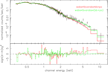
Figure 2: Coadded EPIC spectra of the ULX on 2001 Aug 08, with the best-fit bb+po and bknpo models (green and red curves, respectively). A metal abundance $Z=0.07\,Z_{\odot}$ was assumed for the intrinsic absorber. See Table 4 for the fit parameters.

3.2 Timing analysis

Short-term variability, significant to $>99$% according to the Kolmogorov-Smirnoff and $\chi^{2}$ tests, is detected at all epochs, except during Rev. 313 (which has a lower signal-to-noise ratio, since the pn camera was not operating). The source exhibits a flaring behaviour, with changes in flux by a factor of $\sim 2$ over $\sim 100$ s (Fig. 3). The flares are most evident in the 2003 observation, with a Kolmogorov-Smirnoff probability of constancy $<10^{-3}$. Here we focus on two important results from this epoch; a detailed timing study of all the other observations will be presented elsewhere.

Comparing the background-subtracted lightcurves in a soft ($0.2$–$1.5$ keV) and hard ($1.5$–$12$ keV) band, we found that the hard flux drops to a value consistent with zero during the dips (Fig. 4, top); in the soft band, a “baseline”, persistent component is always present in addition to the flaring component (Fig. 4, middle). The rms fractional variability is $\approx 70\%$ in the hard band, and $\approx 30\%$ in the soft band. There is no time lag between the flares in the two bands, suggesting that we are seeing the same variable physical component in both.

The flaring behaviour in the two bands has a simple interpretation in the framework of the bb+po spectral model (Sect. 3.1). In the hard band, the variability is necessarily due to the power-law component: there is no contribution from the thermal component in this band. A change in the power-law component would also affect the soft band, where the power-law and thermal fluxes are of the same order of magnitude. Hence, we suggest that the lightcurves can be explained by a flaring behaviour of the power-law component, while the thermal component does not vary on these short timescales, and represents the baseline flux seen in the soft band.

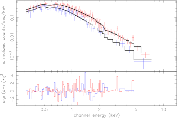
Figure 6: Coadded EPIC spectra of the ULX on 2001 Jan 28, separated into the “low-flux” and “high-flux” states (blue and red datapoints, respectively). See text for details. The spectra are well fitted by a bb+po model: we argue that the blackbody component is consistent with being unchanged in the two states, while the variability is due to the power-law component. A metal abundance $Z=0.07\,Z_{\odot}$ was assumed for the intrinsic absorber. See Table 8 for the fit parameters.

To test our hypothesis, we analysed the lightcurve in the $0.2$–$12$ keV band (Fig. 3, bottom): we divided the exposure into a “low” interval, consisting of all the 50-s bins in which the count rate was $<1$ ct s^-1, and a “high” interval, for rates $>1$ ct s^-1. We then extracted and analysed the combined EPIC spectra from the two sub-intervals; as before, only the $0.3$–$12$ keV band was used for spectral fitting. This choice of threshold is purely arbitrary: we needed to have enough counts in both “states” for a meaningful spectral analysis. We examined whether the change in flux between the peaks and the troughs could simply be modelled with a constant factor, or whether there was also a significant spectral change. We find (Fig. 6; Tables 7, 8) that the blackbody component is consistent with being constant between the two states: the flux variations are consistent with being entirely due to a change in the power-law normalisation, in agreement with our initial hypothesis. In conclusion, we suggest that the ULX exhibits soft dips over timescales of $\sim 10^{2}$ s in which the power-law component is suppressed.

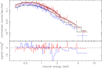
Figure 7: Same datapoints as in Fig. 6. The fitted bb+po model shows that the change in flux between low and high states cannot be due simply to a normalization factor: the spectrum in the low state is softer.

We also fitted the two flux-dependent spectra with a bknpo model (Table 9). The model provides an equally good fit for this particular observations, as shown earlier (Tables 3, 5, 6). However, its physical interpretation is less straightforward. It requires a very high power-law index below the break ($\Gamma_{1}\approx-1$ below $E_{\rm br}\approx 0.55$ keV), thus making the soft component practically indistinguishable from a thermal component over the XMM-Newton/EPIC energy band. In this scenario, the flaring behaviour would correspond to a flattening of the high-energy power-law: from $\Gamma_{2}\approx-3.2$ in the low state to $\Gamma_{2}\approx-2.8$ in the high state Finally, we show (Fig. 7) that the difference between low and high states cannot be due simply to a normalisation factor. The low state is indeed softer (consistent with our interpretation).

To investigate further the characteristic variability timescales, we examined the power spectral density for the 2003 lightcurve; we normalised the Fourier transform to be the squared rms fractional variability per unit frequency. Firstly, we considered in our analysis only the first uninterrupted 3 ks of the exposure (Fig. 4); then we considered the power spectrum for the whole exposure, filling the two data gaps with a running mean. We obtained similar results. The power spectrum for the full-band lightcurve (Fig. 5) has a slope $\alpha=-1.3\pm 0.2$ over two decades in frequency ($3\times 10^{-3}\la\nu\la 0.3$ Hz); it peaks at $\nu_{\rm b}\approx 2.5\times 10^{-3}$ Hz, and is flat (consistent with $\alpha=0$) at lower frequencies. The power spectrum for the hard-band lightcurve has similar features, with a break at $\nu_{\rm b}\approx 3\times 10^{-3}$ Hz and a slope $\alpha=-0.9\pm 0.4$ at higher frequencies.

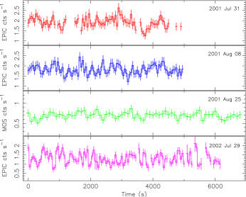
Figure 3: Coadded EPIC lightcurves of the ULX over the four observations of 2001–2002.

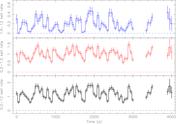
Figure 4: Coadded EPIC lightcurves of the ULX in 2003 Jan (Rev. 574), rebinned to 50 s. Top panel: $1.5$–$12$ keV band; medium panel: $0.2$–$1.5$ keV band; bottom panel: full $0.2$–$12$ keV band.

Figure 5: Power density spectrum of the source in 2003 Jan, normalised to give the squared rms fractional variability per unit frequency; the expected white noise level has been subtracted. Only the first, uninterrupted 3 ks of the exposure have been used for this spectrum; however, very similar results are obtained when we used the whole exposure.

Table 7: Best-fit parameters for a bb+po simultaneous fit to the combined EPIC spectra in the “low” and “high” intervals of the 2003 Jan observation. As before, the quoted errors are the 90% confidence limit and $n_{\rm H,Gal}=5.7\times 10^{20}$ cm^-2. We assumed a solar abundance for the intrinsic absorber ($Z=Z_{\odot}$).

Parameter	“Low” value	“High” value
model: wabs${}_{\rm Gal}\leavevmode\nobreak\ \times$ wabs $\times$ (bb $+$ po)
$n_{\rm H}\leavevmode\nobreak\ (10^{21}\leavevmode\nobreak\ {\rm cm}^{-2})$	$(1.4^{+0.5}_{-0.3})$	$(1.4^{+0.5}_{-0.3})\leavevmode\nobreak\ ^{\mathrm{(a)}}$
$kT_{\rm bb}\leavevmode\nobreak\ ({\rm keV})$	$0.11^{+0.02}_{-0.01}$	$0.12^{+0.01}_{-0.02}$
$K_{\rm bb}\leavevmode\nobreak\ (10^{-5})$	$3.7^{+3.1}_{-0.9}$	$3.9^{+4.8}_{-1.0}$
$\Gamma$	$2.86^{+0.42}_{-0.37}$	$2.68^{+0.19}_{-0.18}$
$K_{\rm po}\leavevmode\nobreak\ (10^{-4})$	$3.1^{+1.0}_{-0.9}$	$6.4^{+1.2}_{-1.2}$
$\chi^{2}_{\nu}$	$0.76\,(137.8/182)$
$f_{0.3{\rm-}12{\rm,\,obs}}\leavevmode\nobreak\ (10^{-12}\leavevmode\nobreak\ {\rm erg\leavevmode\nobreak\ cm}^{-2}\leavevmode\nobreak\ {\rm s}^{-1})$	$1.1^{+0.2}_{-0.4}$	$2.0^{+0.2}_{-0.4}$
$f_{0.3{\rm-}12}\leavevmode\nobreak\ (10^{-12}\leavevmode\nobreak\ {\rm erg\leavevmode\nobreak\ cm}^{-2}\leavevmode\nobreak\ {\rm s}^{-1})$	$3.6^{+0.4}_{-1.9}$	$5.5^{+0.3}_{-2.3}$
$f^{\mathrm{bb}}_{0.3{\rm-}12}\leavevmode\nobreak\ (10^{-12}\leavevmode\nobreak\ {\rm erg\leavevmode\nobreak\ cm}^{-2}\leavevmode\nobreak\ {\rm s}^{-1})$	$2.1^{+0.7}_{-1.6}$	$2.3^{+1.1}_{-2.0}$
$f^{\mathrm{po}}_{0.3{\rm-}12}\leavevmode\nobreak\ (10^{-12}\leavevmode\nobreak\ {\rm erg\leavevmode\nobreak\ cm}^{-2}\leavevmode\nobreak\ {\rm s}^{-1})$	$1.5^{+1.2}_{-0.4}$	$3.1^{+1.3}_{-0.6}$
$L_{0.3{\rm-}12}\leavevmode\nobreak\ (10^{40}\leavevmode\nobreak\ {\rm erg\leavevmode\nobreak\ s}^{-1})$	$1.0$	$1.8$

• assumed to be equal for the two states

Table 8: As in Table 7, but with $Z=0.07\,Z_{\odot}$.

Parameter	“Low” value	“High” value
model: wabs${}_{\rm Gal}\leavevmode\nobreak\ \times$ tbvarabs $\times$ (bb $+$ po)
$n_{\rm H}\leavevmode\nobreak\ (10^{21}\leavevmode\nobreak\ {\rm cm}^{-2})$	$(1.6^{+0.7}_{-0.4})$	$(1.6^{+0.7}_{-0.4})\leavevmode\nobreak\ ^{\mathrm{(a)}}$
$kT_{\rm bb}\leavevmode\nobreak\ ({\rm keV})$	$0.11^{+0.02}_{-0.01}$	$0.12^{+0.01}_{-0.02}$
$K_{\rm bb}\leavevmode\nobreak\ (10^{-5})$	$1.9^{+1.8}_{-0.9}$	$1.7^{+1.9}_{-0.8}$
$\Gamma$	$2.88^{+0.42}_{-0.37}$	$2.66^{+0.18}_{-0.19}$
$K_{\rm po}\leavevmode\nobreak\ (10^{-4})$	$3.0^{+0.9}_{-0.7}$	$6.0^{+1.0}_{-0.8}$
$\chi^{2}_{\nu}$	$0.72\,(130.9/182)$
$f_{0.3{\rm-}12{\rm,\,obs}}\leavevmode\nobreak\ (10^{-12}\leavevmode\nobreak\ {\rm erg\leavevmode\nobreak\ cm}^{-2}\leavevmode\nobreak\ {\rm s}^{-1})$	$1.1^{+0.2}_{-0.3}$	$2.0^{+0.2}_{-0.3}$
$f_{0.3{\rm-}12}\leavevmode\nobreak\ (10^{-12}\leavevmode\nobreak\ {\rm erg\leavevmode\nobreak\ cm}^{-2}\leavevmode\nobreak\ {\rm s}^{-1})$	$2.6^{+0.8}_{-0.3}$	$4.0^{+0.9}_{-0.4}$
$f^{\mathrm{bb}}_{0.3{\rm-}12}\leavevmode\nobreak\ (10^{-12}\leavevmode\nobreak\ {\rm erg\leavevmode\nobreak\ cm}^{-2}\leavevmode\nobreak\ {\rm s}^{-1})$	$1.1^{+0.5}_{-0.2}$	$1.0^{+0.7}_{-0.1}$
$f^{\mathrm{po}}_{0.3{\rm-}12}\leavevmode\nobreak\ (10^{-12}\leavevmode\nobreak\ {\rm erg\leavevmode\nobreak\ cm}^{-2}\leavevmode\nobreak\ {\rm s}^{-1})$	$1.5^{+0.3}_{-0.2}$	$3.0^{+0.3}_{-0.3}$
$L_{0.3{\rm-}12}\leavevmode\nobreak\ (10^{40}\leavevmode\nobreak\ {\rm erg\leavevmode\nobreak\ s}^{-1})$	$0.7$	$1.1$

• assumed to be equal for the two states

Table 9: As in Table 6 and 7, for a bknpo model. We assumed $Z=0.07\,Z_{\odot}$.

Parameter	“Low” value	“High” value
model: wabs${}_{\rm Gal}\leavevmode\nobreak\ \times$ tbvarabs $\times$ bknpo
$n_{\rm H}\leavevmode\nobreak\ (10^{21}\leavevmode\nobreak\ {\rm cm}^{-2})$	$(<0.6)$	$(<0.6)\leavevmode\nobreak\ ^{\mathrm{(a)}}$
$\Gamma_{1}$	$-1.1^{+2.4}_{-1.8}$	$-1.3^{+2.0}_{-0.2}$
$E_{\rm br}\leavevmode\nobreak\ ({\rm keV})$	$0.55^{+0.09}_{-0.05}$	$0.56^{+0.06}_{-0.05}$
$\Gamma_{2}$	$3.25^{+0.21}_{-0.16}$	$2.79^{+0.12}_{-0.08}$
$K_{\rm bp}\leavevmode\nobreak\ (10^{-3})$	$4.9^{+10.1}_{-3.9}$	$7.1^{+13.5}_{-5.0}$
$\chi^{2}_{\nu}$	$0.75\,(137.1/182)$
$f_{0.3{\rm-}12{\rm,\,obs}}\leavevmode\nobreak\ (10^{-12}\leavevmode\nobreak\ {\rm erg\leavevmode\nobreak\ cm}^{-2}\leavevmode\nobreak\ {\rm s}^{-1})$	$1.0^{+0.1}_{-0.1}$	$2.0^{+0.1}_{-0.1}$
$f_{0.3{\rm-}12}\leavevmode\nobreak\ (10^{-12}\leavevmode\nobreak\ {\rm erg\leavevmode\nobreak\ cm}^{-2}\leavevmode\nobreak\ {\rm s}^{-1})$	$1.4^{+0.2}_{-0.1}$	$2.4^{+0.4}_{-0.1}$
$L_{0.3{\rm-}12}\leavevmode\nobreak\ (10^{40}\leavevmode\nobreak\ {\rm erg\leavevmode\nobreak\ s}^{-1})$	$0.4$	$0.7$

• assumed to be equal for the two states

4 Conclusions

Our spectral analysis, based on five XMM-Newton/EPIC observations between 2001 July and 2003 January, shows a thermal component with $kT_{\rm bb}\approx 0.12$–$0.14$ keV, significantly detected at all epochs, in addition to a soft power-law ($\Gamma\approx 2.6$–$2.9$). A broken power-law model, as suggested in Kaaret et al. (2003), is acceptable at some epochs, but is not consistent with the full series of observations, and is generally worse than a blackbody plus power-law model or a Comptonised blackbody model.

Ruling out a simple broken power-law model does not rule out the possibility that the X-ray emission is due to inverse-Compton emission from a jet, enhanced by relativistic Doppler boosting (Kaaret et al. 2003). It was suggested in Georganopoulos (2002), and Georganopoulos & Kazanas (2003), that a more realistic jet spectrum would have a curvature around the break energy, thus mimicking a soft thermal component. Spectral analysis over a larger energy range is required to test this possibility.

In any case, the X-ray spectrum is consistent with a more massive accreting BH in a high/soft or very high state. Given its inferred isotropic luminosity of $\approx 10^{40}$ erg s^-1 in the $0.3$–$12$ keV band, a mass $\ga 100M_{\odot}$ is required to satisfy the Eddington limit. Thus, the ULX in NGC 5408 appears very similar to a group of “canonical” ULXs in nearby dwarf and spiral galaxies, with a low-temperature thermal component at $kT_{\rm bb}\sim 0.1$ keV and emitted luminosity $\sim(1$–$2)\times 10^{40}$ erg s^-1. In all these systems, if the soft thermal component is interpreted as the emission from the inner part of a standard accretion disk (Shakura & Sunyaev 1973), its temperature would imply masses $>10^{5}M_{\odot}$, unphysically high for a non-nuclear BH. However, it was also suggested (King 2003) that these ULXs may be accreting BHs during a super-Eddington accretion phase: they could have a luminosity close or even a factor of a few above the Eddington limit, accompanied by a radiatively-driven, Compton-thick outflow from the accretion disk. In this scenario, the soft thermal component would come from the photosphere of the outflow. Hence, the BH mass would not need to be higher than $\sim 20$–$50M_{\odot}$, still consistent with a stellar origin.

We note that this ULX is located in a very metal-poor dwarf galaxy ($Z\approx 0.07Z_{\odot}$). An association between ULXs and metal-poor environments was suggested by Pakull & Mirioni (2002). Low metal abundance implies a reduced mass-loss rates in the radiatively-driven wind from the O-star progenitor ($\dot{M}_{\rm w}\sim Z^{0.85}$: Vink et al. 2001; see also Bouret et al. 2003); this leads to a more massive stellar core, which may then collapse into a more massive BH, via normal stellar evolution. Hence, low abundances may explain the formation of isolated BHs with masses up to $\approx 50M_{\odot}$ (ie, up to $\approx$ half of the mass of the progenitor star).

We found a moderate long-term spectral variability between the various epochs of the XMM-Newton observations, with a ratio between the maximum and minimum fluxes of $\approx 1.4$. This is consistent with the long-term behaviour of the source from previous Einstein, ROSAT, ASCA and Chandra observations (Kaaret et al. 2003). Our preliminary timing analysis shows rapid variability and flaring-like behaviour, particularly in the 2003 Jan observation. The variability is larger in the hard band ($E>1.5$ keV), where the flux is consistent with zero during the dips.

The bb+po spectral model offers a clean, simple interpretation of the flaring behaviour. In this scenario, we have interpreted the lightcurves as the combination of a rapidly variable power-law component, plus an additional, non-variable thermal component below 1.5 keV, consistent with our spectral analysis. The power-law flux appears to be suppressed during the dips, when the X-ray spectrum becomes softer; this is supported by flux-dependent spectral analysis. The power-law X-ray emission in accreting BH binaries is generally explained as inverse-Compton scattering of soft disk photons in a hot corona or Compton cloud, located either above the inner part of the accretion disk, or as a quasi-spherical region inside the truncation radius of the disk.

A flaring behaviour with soft dips or transitions has also been observed in Galactic microquasars such as GRS 1915$+$105 (Naik et al. 2001) and, in one case, XTE J1550$-$564 (Rodriguez et al. 2003). It was interpreted (Vadawale et al. 2003) as evidence that the matter responsible for the Comptonised component is recurrently ejected from the inner regions; the ejected matter may be responsible for the optically-thin synchrotron radio emission in those systems. A more detailed discussion of this hypothesis, and of whether it may explain the steep-spectrum radio emission detected by the Australia Telescope Compact Array at the position of the ULX (Kaaret et al. 2003; Stevens et al. 2002), will be addressed in further work.

The power density spectrum for this ULX is flat below $\approx 2.5$ mHz, and has a slope of $\approx-1$ at higher frequencies. This is similar to what is found in “canonical” Galactic BH candidates and AGN: it is believed that the break frequency is inversely proportional to the mass of the accreting BH (eg, Belloni & Hasinger 1990; Nowak et al. 1999; Uttley et al. 2002; Markowitz et al. 2003; Cropper et al. 2004). For example, the break in the power density spectrum of Cyg X-1 occurs at $\nu\sim 0.4$–$0.04$ Hz in different accretion states (Nowak et al. 1999). This suggests that the mass of the BH powering the ULX in NGC 5408 is $\sim 10^{2}M_{\odot}$. This is also in good agreement with the inferred luminosity, if we require that it does not exceed the Eddington limit. Such a high mass would rule out (cf. Fig. 3 of Kaaret et al. 2004) an association of this ULX with the young star clusters in the starburst region of NGC 5408, located $\approx 300$ pc to the north-west. However, we are aware that the relation between break frequency and BH mass is very uncertain, and the power-density spectra are often more complicated than a simple broken power law (see, eg, the case of GRS 1915$+$105: Morgan et al. 1997).

In conclusion, we argue that both the spectral and timing results from our XMM-Newton study are consistent with the possibility that this ULX is at the upper end of the mass range for BHs of stellar origin, a few times more massive than “standard” BH candidates such as Cyg X-1. In that case, its luminosity would be very close or, more likely, slightly higher than its Eddington limit, and a strong outflow would be expected from its accretion disk. Doppler boosting in a relativistic jet is not required to explain the observed properties, although we cannot rule it out.

- (1)
- (2) Arnaud, K. A. 1996, Astronomical Data Analysis Software and Systems V, ASP Conf. Series, 101, 17
- (3) Belloni, T. 2001, preprint (astro-ph/0112217)
- (4) Belloni, T., & Hasinger, G. 1990, A&A, 227, L33
- (5) Blackburn, J. K. 1995, Astronomical Data Analysis Software and Systems IV, ASP Conference Series, 77, 367
- (6) Bouret, J.-C., Lanz, T., Hillier, D. J., et al. 2003, ApJ, 595, 1182
- (7) Colbert, E. J. M., & Mushotsky, R. F. 1999, ApJ, 519, 89
- (8) Cropper, M. S., Soria, R., Mushotzky, R. F., et al. 2004, MNRAS, 349, 39
- (9) Dewangan, G. C., Miyaji, T., Griffiths, R. E., & Lehmann, L. 2004, ApJ, submitted (astro-ph/0401223)
- (10) Dickey, J. M., & Lockman, F. J. 1990, ARA&A, 28, 215
- (11) Fabbiano, G. 1992, ARA&A, 27, 87
- (12) Fabian, A. C., & Ward, M. J. 1993, MNRAS, 263, L51
- (13) Georganopoulos, M., Aharonian, F. A., & Kirk, J. G. 2002, A&A, 388, L25
- (14) Georganopoulos, M., & Kazanas, D. 2003, ApJ, 589, L5
- (15) Hamilton, W. C. 1965, Acta Cryst., 18, 502
- (16) Himmelblau, D. M. 1970, Process Analysis by Statistical Methods, New York: John Wiley, pp. 214–222
- (17) Kaaret, P., Corbel, S., Prestwich, A. H., & Zezas, A. 2003, Science, 299, 365
- (18) Kaaret, P., et al. 2004, MNRAS, 348, L2
- (19) Karachentsev, I. D., Sharina, M. E., Dolphin, A. E., et al. 2002, A&A, 385, 21
- (20) King, A. R. 2002, MNRAS, 335, L13
- (21) King, A. R. 2003, in the Proc. of the 2nd BeppoSAX Meeting: ”The Restless High-Energy Universe” (Amsterdam, May 5-8, 2003), E. P. J. van den Heuvel, J. J. M. in ’t Zand, and R. A. M. J. Wijers Eds, astro-ph/0309524
- (22) Körding, E., Falcke, H., & Markoff, S. 2002, A&A, 382, L13
- (23) Madau, P., & Rees, M. J. 2001, ApJ, 551, L27
- (24) Markowitz, A., Edelson, R., Vaughan, S., et al. 2003, ApJ, 593, 96
- (25) Miller, J. M., Fabbiano, G., Miller, M. C., & Fabian, A. C. 2003, ApJ, 585, L37
- (26) Morgan, E. H., Remillard, R. A., & Greiner, J. 1997, ApJ, 482, 993
- (27) Naik, S., Agrawal, P. C., Rao, A. R., et al. 2001, ApJ, 546, 1075
- (28) Nowak, M. A., Vaughan, B. A., Wilms, J., Dove, J. B., & Begelman, M. C. 1999, ApJ, 510, 874
- (29) Page, M. J., Davis, S. W., & Salvi, N. J. 2003, MNRAS, 343, 1241
- (30) Pakull, M. W., & Mirioni, L. 2002, to appear in the proceedings of the symposium ’New Visions of the X-ray Universe’, 26-30 November 2001, ESTEC, The Netherlands (astro-ph/0202488)
- (31) Prince, E. 1982, Acta Cryst., B38, 1099
- (32) Portegies Zwart, S. F., Baumgardt, H., Hut, P., Makino, J., & McMillan, S. L. W. 2004, Nature, in press (astro-ph/0402622)
- (33) Roberts, T. P., & Warwick, R. S. 2000, MNRAS, 315, 98
- (34) Rodriguez, J., Corbel, S., & Tomsick, J. A. 2003, ApJ, 595, 1032
- (35) Shakura, N. I., & Sunyaev, R. A. 1973, A&A, 24, 337
- (36) Shrader, C. R., & Titarchuk, L. G. 1999, ApJ, 521, L21
- (37) Stevens, I. R., Forbes, D. A., & Norris, R. P. 2002, MNRAS, 335, 1079
- (38) Stewart, G. C., Fabian, A. C., Terlevich, R. J., & Hazard, C. 1982, MNRAS, 200, 61P
- (39) Uttley, P., McHardy, I. M., & Papadakis, I. E. 2002, MNRAS, 332, 231
- (40) Vadawale, S. V., Rao, A. R., Naik, S., et al. 2003, ApJ, 597, 1023
- (41) Vink, J. S., de Koter, A., & Lamers, H. J. G. L. M. 2001, A&A, 369, 574
- (42) Williams, E. J., & Kloot, N. H. 1953, Aust. J. Appl. Sci., 4, 1
- (43) Wilms, J., Allen, A., & McCray, R. 2000, ApJ, 542, 914