Dark Energy Search with Supernovae

Abstract

To determine the nature of dark energy from observational data, it is important that we use model-independent and optimal methods. We should probe dark energy using its density (allowed to be a free function of cosmic time) instead of its equation of state. We should minimize gravitational lensing effect on supernovae by flux-averaging. We need to include complementary data (for example, from the Cosmic Microwave Background [CMB] and large scale structure [LSS]) in a consistent manner to help break the degeneracy between the dark energy density and the matter density fraction. We should push for ambitious future supernova surveys that can observe a large number of supernovae at the highest possible redshifts. I discuss these and other issues that will be important in our quest to unravel the mystery of the nature of dark energy.

Current supernova, CMB, and LSS data already rule out dark energy models with dark energy densities that vary greatly with time; with the cosmological constant model providing an excellent fit to the data. A precise measurement of dark energy density as a free function of cosmic time will have a fundamental impact on particle physics and cosmology.

1 Introduction

The data of type Ia supernovae (SNe Ia) reveal that the expansion of our universe is accelerating [Riess et al. 1998, Perlmutter et al. 1999]. This implies the existence of dark energy. Solving the mystery of the nature of dark energy will have revolutionary implications in particle physics and cosmology.

The first most fundamental question about dark energy is whether the dark energy density depends on time. The time dependence of the dark energy density can be used to distinguish the various models. [Freese 2004]

A powerful probe of dark energy is SNe Ia, which can be calibrated to be good cosmological standard candles [Phillips 1993, Riess, Press, & Kirshner 1995, Branch 1998], and used to measure how distance changes with redshift. For a flat universe, the luminosity distance is

$$d_{L}(z) = cH_{0}^{-1}(1+z)\int_{0}^{z}\frac{dz^{\prime}}{E(z^{\prime})},$$

$$E(z) = \left[\Omega_{m}(1+z)^{3}+(1-\Omega_{m})\rho_{X}(z)/\rho_{X}(0)\right]^{1/2},$$ (1)

where $\rho_{X}(z)$ is the dark energy density. Note that dark nergy only appears in the form of the function $E(z)$; $\rho_{X}(z)$ is on the same footing as the matter density fraction $\Omega_{m}$ in the context of observational tests. The dark energy equation of state is [Wang & Garnavich 2001]

$$w_{X}(z)=\frac{p_{X}(z)}{\rho_{X}(z)}=\frac{(1+z)}{3}\frac{\rho_{X}^{\prime}(z)}{\rho_{X}(z)}-1.$$ (2)

2 Probing Dark Energy Using Its Density Instead of Its Equation of State

Due to the integrals and parameter degeneracies in the distance-redshift relations of standard candles (see Eq.[1]), it is very difficult to detect the time-dependence of the dark energy equation of state $w_{X}(z)$ in a model-independent manner from realistic data [Maor, Brustein, & Steinhardt 2001, Barger & Marfatia 2001]. By measuring the dark energy density $\rho_{X}(z)$, instead of $w_{X}(z)$, we effectively remove one integral, and increase the likelihood to detect the evolution of dark energy. [Wang & Garnavich 2001, Tegmark 2002] This would allow us to determine whether dark energy is vacuum energy, or some other form of exotic energy.

It is easier to extract $\rho_{X}(z)$ from the data than to extract $w_{X}(z)$. This is easy to see mathematically: to obtain $\rho_{X}(z)$, take a single derivative of data (see Eq.[1]); to obtain $w_{X}(z)$, we need to take a second derivative (see Eq.[2]).

Fig.1 explicitly demonstrates the advantage of the $\rho_{X}(z)$ parametrization over the $w_{X}(z)$ parametrization, using recent observational data. Fig.1 shows $\rho_{X}(z)$ and $w_{X}(z)$ measured from 192 SNe Ia from the Tonry/Barris sample [Tonry et al. 2003, Barris et al. 2004], flux-averaged with $\Delta z=0.05$, and combined with CMB (shift parameter $R_{0}=1.716\pm 0.062$ [Spergel et al. 2003]) and LSS data (growth parameter $f_{0}\equiv f(z=0.15)=0.51\pm 0.11$ [Hawkins et al. 2003, Verde et al. 2002]). The solid and dashed lines enclose the 68.3% and 95% confidence regions respectively.[Wang & Mukherjee 2004, Wang & Freese 2004]

Figure 1: $w_{X}(z)$ and $\rho_{X}(z)$ measured from 192 SNe Ia from the Tonry/Barris sample, flux-averaged, and combined with CMB (shift parameter $R_{0}=1.716\pm 0.062$) and LSS (growth parameter $f_{0}\equiv f(z=0.15)=0.51\pm 0.11$) data.

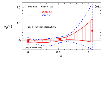
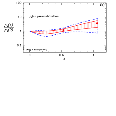
Note that $\rho_{X}(z)$ is more tightly constrained than $w_{X}(z)$. [Daly & Djorgovski 2004] and [Huterer & Cooray 2004] found similar results using a different sample of SNe Ia (the Riess sample).

While using $\rho_{X}(z)$ in the likelihood analysis of data encompasses all possible dark energy models, using $w_{X}(z)$ implies $\rho_{X}(z)\geq 0$ since $\rho_{X}(0)>0$ (see Eq.[2]). To allow for exotic origins of dark energy, we should not impose a positive prior on the dark energy density. This again argues in favor of using $\rho_{X}(z)$ instead of $w_{X}(z)$ to probe dark energy.[Wang & Tegmark 2004]

3 Go Deep: the Optimal SN Observational Strategy for Probing Dark Energy Evolution

To determine whether SNe Ia are good cosmological standard candles, we need to nail the systematic uncertainties (luminosity evolution, gravitational lensing, dust) [Aldering 2004]. This will require at least hundreds of SNe Ia at $z>1$. This can be easily accomplished by doing a supernova pencil beam survey using a dedicated telescope, which can be used for other things simultaneously (weak lensing, gamma ray burst afterglows, etc) [Wang 2000a].

The inclusion of a large number of SNe Ia at high redshifts is important for probing the time evolution of dark energy density. Fig.2 shows that a shallow and wide survey (the survey strategy for SNAP as of 2001) compares poorly with a supernova pencil beam survey in constraining dark energy density at high $z$ [Wang & Lovelace 2001].

Figure 2: A shallow and wide survey (the original survey strategy for SNAP) compares poorly with a supernova pencil beam survey in constraining dark energy density at high $z$ [Wang & Lovelace 2001].

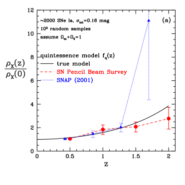
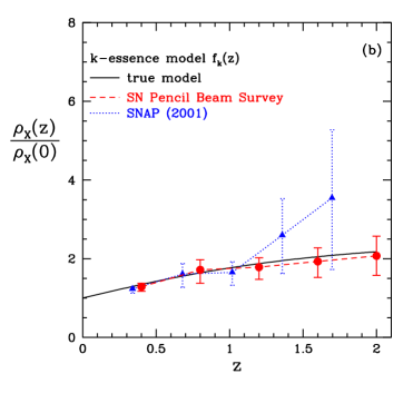
Clearly, in order to probe time evolution of dark energy density, it is essential to conduct a SN survey that is as deep as feasible, so that the largest possible number of SNe Ia at high redshifts can be observed.

4 Data Analysis Method

Here is a recipe for optimally extracting dark energy density $\rho_{X}(z)$ from observational data [Wang & Mukherjee 2004]:
1) Obtain SN Ia peak brightnesses with uncertainties in flux.
2) Parametrize $\rho_{X}(z)$ as a free function (given by $\rho_{X}(z_{i})/\rho_{X}(0)$, $i=1,2,...,N$, and interpolated elsewhere). Additional parameters are $\Omega_{m}$ and $H_{0}$.
3) Use flux-averaging statistics in computing $\chi^{2}$ of SN Ia data [Wang 2000b].
4) Add other data (CMB, LSS) to help constrain $\Omega_{m}$.[Knop et al. 2003]
5) Use Markov Chain Monte Carlo (MCMC) to find marginalized probability distributions of estimated parameters.

I will highlight the need for flux-averaging of supernovae and the advantage of MCMC below.

4.1 Minimizing gravitational lensing effect on SNe Ia by flux-averaging

Since our universe is inhomogeneous in matter distribution, the apparent brightness of SNe Ia can be altered by the intervening matter distribution. [Wang, Holz, & Munshi 2002] gives a universal probability distribution for weak lensing magnification of SNe Ia. Because lensing only redistributes the light (flux) from the SNe Ia, the effect of weak lensing on supernovae can be minimized by flux-averaging. Therefore, flux-averaging justifies the use of the distance-redshift relation for a smooth universe in the analysis of SN Ia data. [Wang 2000b].

For $\chi^{2}$ statistics using MCMC or a grid of parameters, here are the steps in flux-averaging:

(1) Convert the distance modulus of SNe Ia, $\mu_{0}(z)$, into “fluxes”

$$F(z_{j})\equiv 10^{-(\mu_{0}(z_{j})-25)/2.5}=\left(\frac{d_{L}^{data}(z)}{\mbox{Mpc}}\right)^{-2}.$$ (3)

(2) For a given set of cosmological parameters $\{{\bf s}\}$, obtain “absolute luminosities”, {${L}(z_{j})$}, by removing the redshift dependence of the “fluxes”, i.e.,

$${L}(z_{j})\equiv d_{L}^{2}(z_{j}|{\bf s})\,F(z_{j}).$$ (4)

(3) Flux-average the “absolute luminosities” {${L}^{i}_{j}$} in each redshift bin $i$ to obtain $\left\{\overline{L}^{i}\right\}$:

$$\overline{L}^{i}=\frac{1}{N}\sum_{j=1}^{N}{L}^{i}_{j}(z^{i}_{j}),\hskip 28.45274pt\overline{z_{i}}=\frac{1}{N}\sum_{j=1}^{N}z^{i}_{j}.$$ (5)

(4) Place $\overline{L}^{i}$ at the mean redshift $\overline{z}_{i}$ of the $i$-th redshift bin, now the binned flux is

$$\overline{F}(\overline{z}_{i})=\overline{L}^{i}/d_{L}^{2}(\overline{z}_{i}|\mbox{\bf s}).$$ (6)

The 1-$\sigma$ error on each binned data point $\overline{F}^{i}$, $\sigma^{F}_{i}$, is taken to be the root mean square of the 1-$\sigma$ errors on the unbinned data points in the $i$-th redshift bin, {$F_{j}^{i}$} ($j=1,2,...,N$), multiplied by $1/\sqrt{N}$ (see [Wang 2000a]).

(5) Apply “flux statistics” to the flux-averaged data, $\left\{\overline{F}(\overline{z}_{i})\right\}$:

$$\chi^{2}(\mbox{\bf s})=\sum_{i}\frac{\left[\overline{F}(\overline{z}_{i})-F^{p}(\overline{z}_{i}|\mbox{\bf s})\right]^{2}}{\sigma_{F,i}^{2}},$$ (7)

where $F^{p}(\overline{z}_{i}|\mbox{\bf s}_{1})=\left(d_{L}(z|\mbox{\bf s})/\mbox{Mpc}\right)^{-2}$.

A Fortran code that uses flux-averaging statistics to compute the likelihood of an arbitrary dark energy model (given the SN Ia data from [Riess et al. 2004]) can be found at $http://www.nhn.ou.edu/\sim wang/SNcode/$ [Wang 2000b, Wang & Mukherjee 2004, Wang & Tegmark 2004].

4.2 Likelihood analysis using Markov Chain Monte Carlo (MCMC)

In a likelihood analysis, we need to find the high confidence region of our parameter space given the data. Traditionally, this is done by using a grid of parameter values that span the allowed parameter space.

Markov Chain Monte Carlo (MCMC) uses the Metropolis algorithm:
(1) Choose a candidate set of parameters, ${\bf s}_{*}$, at random from a proposal distribution.
(2) Accept the candidate set of parameters with probability $A({\bf s},{\bf s}_{*})$; otherwise, reject it.

For Gaussian distributed observables, the acceptance function

$$A({\bf s},{\bf s}_{*})=\min\left\{1,\exp\left[-\chi^{2}({\bf s}_{*})+\chi^{2}({\bf s})\right]\right\}.$$ (8)

For sufficient sampling, the true probability density functions (pdf’s) are recovered. See [Neil 1993] for a review of MCMC.

MCMC is much faster than the grid method, and scales linearly with the number of parameters. It gives smooth probability density functions (pdf’s) for estimated parameters since they receive contribution from all MCMC samples (each with a random set of parameter values). Public software containing MCMC is available [Lewis & Bridle 2002].

5 Status and Outlook

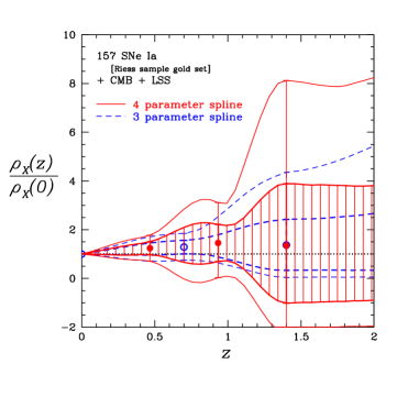
Using the latest SN Ia data, the Riess sample [Riess et al. 2004], which contains 6 SNe Ia at $z>1.25$, together with CMB and LSS data, [Wang & Tegmark 2004] obtained the most accurate measurements to date of the dark energy density $\rho_{X}$ as a free function of cosmic time (see left panel of Fig.3). The solid lines indicate the 68% (shaded) and 95% confidence regions of $\rho_{X}(z)$ parametrized by its values at $z=0.467,0.933,1.4$ (splined elsewhere for $z<1.4$). The thick and thin dashed lines indicate the estimated $\rho_{X}(z)$ parametrized by its values at $z=0.7,1.4$ (splined elsewhere for $z<1.4$). A powerlaw form of $\rho_{X}(z)$ is assumed at $z>1.4$ (where there are only two observed SNe Ia); this allows the CMB and LSS constraints to be included in a self-consistent manner. This is important since it is incorrect (although common practice) to include priors on $\Omega_{m}$ derived assuming $\rho_{X}(z)/\rho_{X}(0)=1$. [Wang & Tegmark 2004] Further, $\rho_{X}(z)$ derived assuming fixed values of $\Omega_{m}$ may be misleading because of the degeneracy between $\rho_{X}(z)$ and $\Omega_{m}$. All our results have been marginalized over $\Omega_{m}$ and $H_{0}$.

Figure 3: Dark energy density $\rho_{X}$ as a free function of cosmic time estimated from supernova, CMB (shift parameter $R_{0}=1.716\pm 0.062$), and LSS (growth parameter $f_{0}\equiv f(z=0.15)=0.51\pm 0.11$) data. Left panel: The latest SN data, with $\rho_{X}$ parametrized by 4 and 3 parameter splines; with estimated $\Omega_{m}=0.278\pm 0.061$ and $\Omega_{m}=0.279\pm 0.053$ respectively. Right panel: The latest SN data (Riess sample) compared to previous data (Tonry/Barris sample, with estimated $\Omega_{m}=0.332\pm 0.062$).

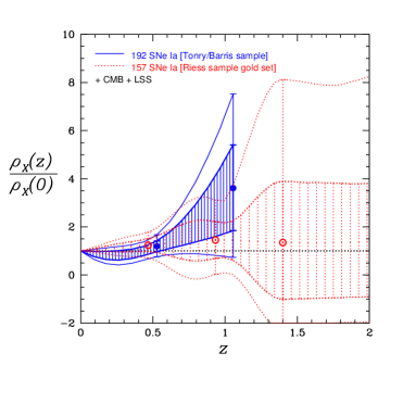
We compare the $\rho_{X}(z)$ estimated from the latest SN data (Riess sample) to that from the previous data (Tonry/Barris sample) in the right panel of Fig.3. Note that the Riess sample gives a substantially tighter constraint on $\rho_{X}(z)$ than the Tonry/Barris sample, and somewhat smaller $\Omega_{m}$. Although the two estimates overlap at the 68% confidence level, the Riess sample clearly favors a dark energy density less dependent on time (with the cosmological constant model giving an excellent fit to the data).

It is interesting that current data already rule out dark energy models with $\rho_{X}(z)$ that vary a lot with time. Future deep supernova surveys on a dedicated telescope will greatly increase the number of observed supernovae [Wang 2000a]. This will allow improved calibration of SNe Ia as cosmological candles, leading to precise measurement of the dark energy density as function of cosmic time, which will have historical impact on particle physics and cosmology.

References

- [Aldering 2004] Aldering, G., this volume.
- [Barger & Marfatia 2001] Barger, V., & Marfatia, D. 2001, Phys. Lett. B, 498, 67
- [Barris et al. 2004] Barris, B.J., et al. 2004, ApJ, 602, 571
- [Branch 1998] Branch, D. 1998, ARA&A, 36, 17
- [Daly & Djorgovski 2004] Daly, R. A., & Djorgovski, S. G. 2004, astro-ph/0403664
- [Freese 2004] Freese, K., this volume.
- [Hawkins et al. 2003] Hawkins, E. et al. 2003, MNRAS, 346, 78
- [Huterer & Cooray 2004] Huterer, D., and Cooray, A., astro-ph/0404062
- [Knop et al. 2003] R. Knop et al. ApJ 598, 102 (2003) ; astro-ph/0309368
- [Lewis & Bridle 2002] Lewis, A., & Bridle, S. 2002, Phys. Rev. D, 66, 103511, astro-ph/0205436
- [Maor, Brustein, & Steinhardt 2001] Maor, I., Brustein, R., & Steinhardt, P.J. 2001, Phys. Rev. Lett., 86, 6
- [Neil 1993] Neil, R.M. 1993, ftp://ftp.cs.utoronto.ca/pub/ radford/review.ps.gz
- [Perlmutter et al. 1999] Perlmutter, S., et al. 1999, ApJ, 517, 565
- [Phillips 1993] Phillips, M.M., ApJ, 413, L105 (1993)
- [Riess, Press, & Kirshner 1995] Riess, A.G., Press, W.H., and Kirshner, R.P., ApJ, 438, L17 (1995)
- [Riess et al. 1998] Riess, A. G., et al. 1998, AJ, 116, 1009
- [Riess et al. 2004] Riess, A. G. et al, 2004, astro-ph/0402512
- [Spergel et al. 2003] Spergel, D. N. et al. 2003, ApJS, 148, 175
- [Tarle et al. 2002] Tarle, G., (for the SNAP Collaboration), astro-ph/0210041
- [Tegmark 2002] Tegmark, M. 2002, Phys. Rev. D66, 103507 [astro-ph/0101354]
- [Tonry et al. 2003] Tonry, J.L., et al. 2003, ApJ, 594, 1
- [Verde et al. 2002] Verde, L. et al. 2002, MNRAS, 335, 432
- [Wang 2000a] Wang, Y. 2000a, ApJ, 531, 676 [astro-ph/9806185]
- [Wang 2000b] Wang, Y. 2000b, ApJ, 536, 531
- [Wang & Freese 2004] Wang, Y., and Freese, K., astro-ph/0402208
- [Wang & Garnavich 2001] Wang, Y., and Garnavich, P. 2001, ApJ, 552, 445
- [Wang, Holz, & Munshi 2002] Wang, Y., Holz, D.E., and Munshi, D. 2002, ApJ, 572, L15
- [Wang & Lovelace 2001] Wang, Y., and Lovelace, G. 2001, ApJ, 562, L115
- [Wang & Mukherjee 2004] Wang, Y., & Mukherjee, P. 2004, astro-ph/0312192, ApJ in press
- [Wang & Tegmark 2004] Wang, Y., & Tegmark, M. 2004, PRL, accepted [astro-ph/0403292]