Stellar Populations and Kinematics of Red Galaxies at $z>2$: Implications for the Formation of Massive Galaxies

Abstract

We recently identified a substantial population of galaxies at $z>2$ with comparatively red rest-frame optical colors. These distant red galaxies (DRGs) are efficiently selected by the simple observed color criterion $J_{s}-K_{s}>2.3$. In this paper we present near-infrared spectroscopy with Keck/NIRSPEC of six DRGs with previously measured redshifts $2.4<z<3.2$, two of which were known to host an active nucleus. We detect continuum emission and emission lines of all observed galaxies. Equivalent widths of H$\alpha$ in the non-active galaxies are 20 Å–30 Å, smaller than measured for Lyman break galaxies (LBGs) and nearby luminous infrared galaxies, and comparable to normal nearby galaxies. The modest equivalent widths imply that the galaxies either have a decreasing star formation rate, or that they are very dusty. Fitting both the photometry and the H$\alpha$ lines, we find continuum extinction $A_{V}=1-2$ mag, ages $1-2.5$ Gyr, star formation rates $200-400\,M_{\odot}$ yr^-1, and stellar masses $1-5\times 10^{11}$ $M_{\odot}$ for models with constant star formation rates. Models with a declining star formation lead to significantly lower extinction, star formation rates, and ages, but similar stellar masses. From [N ii] / H$\alpha$ ratios we infer that the metallicities are high, $1-1.5\times$ Solar. For four galaxies we can determine line widths from the optical emission lines. The widths are high, ranging from $130$ km s^-1 to 240 km s^-1, and by combining data for LBGs and DRGs we find significant correlations between linewidth and restframe $U-V$ color, and between linewidth and stellar mass. The latter correlation has a similar slope and offset as the “baryonic Tully-Fisher relation” for nearby galaxies. From the linewidths and effective radii we infer dynamical masses and mass-to-light ($M/L$) ratios. The median dynamical mass is $\sim 2\times 10^{11}\,M_{\odot}$, supporting the high stellar masses inferred from the photometry. We find that the median $M/L_{V}\approx 0.8\,(M/L)_{\odot}$, a factor of $\sim 5$ higher than measured for LBGs. We infer from our small sample that DRGs are dustier, more metal rich, more massive, and have higher ages than $z\approx 3$ LBGs of the same rest-frame $V$-band luminosity. Although their volume density is still uncertain, their high $M/L$ ratios imply that they contribute significantly to the stellar mass density at $z\approx 2.5$. As their stellar masses are comparable to those of early-type galaxies they may have already assembled most of their final mass.

1 Introduction

It is still not known how and when massive galaxies were formed. Early studies envisioned an epoch of rapid collapse at high redshift, followed by sustained star formation in a disk and a smooth and regular dimming of the stellar light in the spheroidal component (e.g., Eggen, Lynden-Bell, & Sandage 1962). More recently, hierarchical galaxy formation models in Cold Dark Matter (CDM) cosmologies have postulated that massive galaxies have complex assembly histories, and were built up gradually through mergers and periods of star formation (White & Frenk 1991). In these models properties such as mass, star formation rate, and morphology are transient, depending largely on the merger history and the time elapsed since the most recent merger (e.g., Kauffmann, White, & Guiderdoni 1993; Kauffmann et al. 1999; Baugh et al. 1998; Meza et al. 2003).

One of the most direct tests of hierarchical galaxy formation models is the predicted decline of the abundance of massive galaxies with redshift. The best studied galaxies at high redshift are $z\approx 3$ Lyman break galaxies (LBGs) (Steidel & Hamilton 1992; Steidel, Pettini, & Hamilton 1995; Steidel et al. 1996). Measurements have been made of their clustering properties (Giavalisco et al. 1998), star formation histories (Papovich, Dickinson, & Ferguson 2001; Shapley et al. 2001), contribution to the cosmic star formation rate (Madau et al. 1996; Steidel et al. 1999; Adelberger & Steidel 2000), rest-frame optical emission lines (Pettini et al. 2001), and interaction with the IGM (Adelberger et al. 2003). Initially LBGs were thought to be very massive (Steidel et al. 1996), but these estimates have been revised following the realization that their rest-frame UV kinematics are dominated by winds rather than gravitational motions (Franx et al. 1997; Pettini et al. 1998). The masses of luminous $z\approx 3$ LBGs appear to be $\sim 10^{10}M_{\odot}$ (Pettini et al. 2001; Shapley et al. 2001), a factor of $\sim 10$ lower than the most massive galaxies today. Such relatively low masses are qualitatively consistent with hierarchical models. LBGs in these models are “seeds” marking the highest density peaks in the early Universe, and form the low mass building blocks of massive galaxies in groups and clusters (e.g., Baugh et al. 1998).

Despite these advances and the qualitative consistency of theory and observations many uncertainties remain. Perhaps most fundamentally, it is still not clear whether LBGs are the (only) progenitors of today’s massive galaxies. The highly successful Lyman break technique selects objects with strong UV emission, corresponding to galaxies with high star formation rates and a limited amount of obscuration of the stellar continuum. Galaxies whose light is dominated by evolved stellar populations, and those that are heavily obscured by dust, may therefore be underrepresented in LBG samples (see, e.g., Francis, Woodgate, & Danks 1997; Stiavelli et al. 2001; Hall et al. 2001; Blain et al. 2002; Franx et al. 2003).

Recent advances in near-infrared (NIR) capabilities on large telescopes have made it possible to select high redshift galaxies in the rest-frame optical rather than the rest-frame UV. The rest-frame optical is much less sensitive to dust extinction and is expected to be a better tracer of stellar mass. The FIRES project (Franx et al. 2003) is the deepest ground-based NIR survey to date, with 101.5 hrs of VLT time invested in a single pointing on the Hubble Deep Field South (HDF-S) (Labbé et al. 2003), and a further 77 hrs on a mosaic of four pointings centered on the foreground cluster MS 1054–03 (van Dokkum et al. 2003; Förster Schreiber et al. 2004).

We have selected high redshift galaxies in the FIRES fields by their observed NIR colors. The simple criterion $J_{s}-K_{s}>2.3$ efficiently isolates galaxies with prominent Balmer- or 4000 Å-breaks at $z>2$ (see Franx et al. 2003). This rest-frame optical break selection is complementary to the rest-frame UV Lyman break selection. We find large numbers of red $z>2$ objects in both fields (Franx et al. 2003; van Dokkum et al. 2003). Surface densities are $\sim 3$ arcmin^-2 to $K_{s}=22.5$ and $\sim 1$ arcmin^-2 to $K_{s}=21$, and the space density is 30–50 % of that of LBGs. Their much redder colors suggest they have higher mass-to-light ($M/L$) ratios, and they may contribute equally to the stellar mass density. Most of the galaxies are too faint in the rest-frame UV to be selected as LBGs. Although the samples are still too small for robust measurements, there are indications that the population is highly clustered (Daddi et al. 2003; van Dokkum et al. 2003; Röttgering et al. 2003). The available evidence suggests they could be the most massive galaxies at high redshift, and progenitors of today’s early-type galaxies.

Although these results are intriguing, large uncertainties remain. The density and clustering measurements are based on very small areas, comprising less than five percent of the area surveyed for LBGs by Steidel and collaborators. Furthermore, owing to their faintness in the observer’s optical, spectroscopic redshifts have been secured for only a handful of objects (van Dokkum et al. 2003). Finally, current estimates of ages, $M/L$ ratios, star formation rates, and extinction are solely based on modeling of broad band spectral energy distributions (SEDs), and as is well known this type of analyis suffers from significant degeneracies in the fitted parameters (see, e.g., Papovich et al. 2001; Shapley et al. 2001).

Confirmation of the high stellar masses and improved constraints on the stellar populations require spectroscopy in the rest-frame optical (the observer’s NIR). Emission lines such as [O iii] $\lambda 4959,5007$ and the Balmer H$\alpha$ and H$\beta$ lines have been studied extensively at low redshift, allowing direct comparisons to nearby galaxies. The H$\alpha$ line is particularly valuable, as its luminosity is proportional to the star formation rate (Kennicutt 1998), and its equivalent width is sensitive to the ratio of current and past star formation activity. When more lines are available metallicity and reddening can be constrained as well. Finally, the widths of rest-frame optical lines better reflect the velocity dispersion of the H ii regions than the widths of rest-UV lines, which are very sensitive to outflows and supernova-driven winds (see, e.g., Pettini et al. 1998).

In this paper, we present NIR spectroscopy of a small sample of $J_{s}-K_{s}$ selected galaxies. Line luminosities, equivalent widths, and linewidths are determined, and the derived constraints on the stellar populations and masses are combined with results from fits to the broad band SEDs. Results are compared to nearby galaxies, and also to LBGs: Pettini et al. (1998, 2001) and Erb et al. (2003) have studied the rest-frame optical spectra of LBGs in great detail, providing an excellent benchmark for such comparisons.

For convenience we use the term distant red galaxies, or DRGs, for galaxies having $J_{s}-K_{s}>2.3$ and redshifts $z\gtrsim 2$. This term is more general than “optical-break galaxies”, as it allows for the possibility that in some galaxies the red colors are mainly caused by dust rather than a strong continuum break. Im et al. (2002) use the designation Hyper Extremely Red Objects, or HEROs, for galaxies with $J-K\gtrsim 2$. However, the corresponding rest-frame optical limits are not really “hyper extreme”, as they would include all but the bluest nearby galaxies: at $z=2.7$, our $J_{s}-K_{s}$ limit corresponds to $U-V\gtrsim 0.1$ in the rest-frame. We use $\Omega_{m}=0.3$, $\Omega_{\Lambda}=0.7$, and $H_{0}=70$ km s^-1 Mpc^-1 (Riess et al. 1998; Spergel et al. 2003). All magnitudes are on the Vega system; AB conversion constants for the ISAAC filters are given in Labbé et al. (2003).

2 Spectroscopy

2.1 Sample Selection and Observations

NIR spectroscopy of high redshift galaxies is more efficient if the redshifts are already known, as that greatly facilitates the search for emission and absorption features. Although “blind” NIR spectroscopy of DRGs should be feasible, for this initial investigation we chose to limit the sample to galaxies of known redshift. By January 2003 (the time of our NIRSPEC observations) redshifts had been measured from the rest-frame UV spectra of seven DRGs at $z>2$. Five are in the field of the $z=0.83$ cluster MS 1054–03, and are presented in van Dokkum et al. (2003). Two are in the Chandra Deep Field South (CDF-S); the rest-frame UV spectra of these galaxies are presented in the Appendix. Of the seven galaxies, two show rest-frame UV lines characteristic of Active Galactic Nuclei (AGN).

Six of the seven DRGs were observed with NIRSPEC (McLean et al. 1998) on Keck II on the nights of 2003 January 21 – 24. The remaining galaxy was given the lowest priority because it is at $z=2.705$, which means that H$\alpha$ and H$\beta$ fall outside the NIR atmospheric windows. NIRSPEC was used in the medium-dispersion mode, providing a plate scale of 2.7 Å pix^-1 in the $H$ band and $4.2$ Å pix^-1 in the $K$ band. The wavelength range offered by the $1024\times 1024$ InSb detector is thus roughly equal to the width of a single NIR atmospheric window. The $0\farcs 76$ slit provides a resolution of 10 Å FWHM in $H$ and 14.5 Å in $K$, corresponding to $\sigma_{\rm instr}\approx 80$ km s^-1 in each band.

The night of January 24 was lost in its entirety due to high winds and fog. The weather was variable January 21 – 23, with strong winds toward the end of each night and the night of January 22 partly cloudy. The seeing was typically $0\farcs 8-1\farcs 0$ in $K$. As conditions varied from mediocre to bad during our four-night run the data presented here are not representative of the full capabilities of NIRSPEC.

The targets were acquired using blind offsets from nearby stars. After an on-target exposure of 900 s the offset was reversed and the star was moved along the slit before offsetting again to the object. This method allows continuous monitoring of slit alignment, which proved to be critical as significant misalignments between slit and setup star were sometimes observed (and corrected). In most cases spectra were obtained at three dither positions (at $0^{\prime\prime}$, $+7^{\prime\prime}$, and $-7^{\prime\prime}$ with respect to center). After each series of dithered observations a nearby bright A0 star was observed with the same setup to enable correction for atmospheric absorption and the detector response function.

Our procedure is similar to that employed by Pettini et al. (2001) and Erb et al. (2003) for LBGs, with one modification: after each reversed offset we obtained a spectrum of the alignment star. Although this extra step further increases already substantial overheads, it is very useful in the data reduction as it provides the spatial coordinate of the (typically very faint) object spectrum in each individual 900 s exposure.

All six galaxies were observed in the NIRSPEC-7 ($K$) filter. For two galaxies we also obtained spectra in the NIRSPEC-4 band (covering their Balmer/4000 Å break regions) and for one of these two we obtained a NIRSPEC-5 ($H$ band) spectrum as well (covering [O iii] and H$\beta$). Overheads were approximately a factor of two; the total science integration time was 10 hours. Integration times and observed wavelength ranges are listed in Table 1.

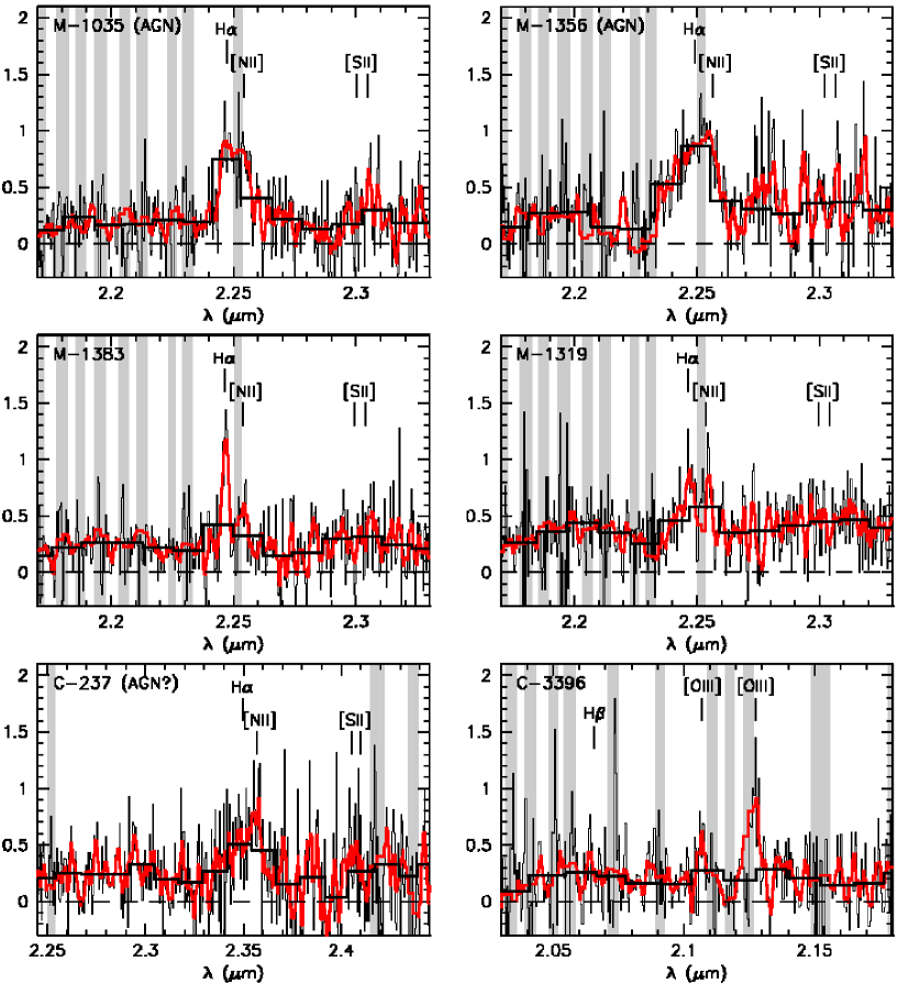
Figure 1: NIRSPEC $K$-band spectra of $J_{s}-K_{s}$ selected galaxies at $z>2$. Black thin lines are raw spectra, black thick histograms are binned spectra, and smoothed spectra are in red. Grey vertical bands denote areas of strong sky emission or absorption; these regions were excluded in the smoothed and binned representations of the data. Emission lines were detected for all galaxies, with typical rest-frame equivalent widths of 20–30 Å. The continuum is also detected in every case.

2.2 Reduction

The data reduction used a combination of standard IRAF tasks and custom scripts. As a first step the strongest cosmic rays were removed, in the following way. The three individual exposures were averaged while rejecting the highest value at each $(x,y)$ position, and the resulting average sky spectrum was subtracted from the raw spectra. The residual spectra are dominated by cosmic rays and sky line residuals resulting from variations in OH line intensities on $\sim 45$ min timescales. The residual spectra were rotated by 85.4 degrees using the IRAF task “rotate” such that the sky line residuals were approximately parallel to columns. Rather than linearly interpolating between pixels we used “nearest” interpolation, so that each pixel in the rotated frame corresponds exactly to a pixel in the original frame (with slight redundancy) and cosmic rays retain their sharp edges. Sky line residuals were subtracted by fitting a third order polynomial along columns. Cosmic rays were identified in each of the three residual images with L.A.Cosmic (van Dokkum 2001), using a 2D noise model created from the subtracted sky spectrum. The cosmic ray frames were rotated back to the original orientation and subtracted from the three raw spectra. We carefully checked by eye that sky lines, pixels adjacent to cosmic rays, and emission lines remained unaffected by the procedure.

Dark current, hot pixels, and a first approximation of the sky spectrum were removed by subtracting the average of the two other dither positions from each cosmic ray cleaned exposure. This procedure increases the noise in each individual image according to $N\approx\sqrt{n/(n-1)}N_{\rm org},$ with $N_{\rm org}$ the noise before sky subtraction and $n$ the number of independent dither positions. The number of dither positions is a trade-off between this noise increase and the effects of variations in atmospheric OH line strengths, dark current, and thermal background on the timescale of the dither sequence. For most of our observations $n=3$, and the increase in the photon noise is $\approx 22$ %.

The frames and their corresponding sky spectra were rotated such that the sky lines are along columns, using a polynomial to interpolate between adjacent pixels. The spectra were wavelength calibrated by fitting Gaussian profiles to the OH lines in the 2D sky spectra. The sky subtracted frames and the sky spectra were rectified to a linear wavelength scale. Sky line residuals were subtracted by fitting a second order polynomial along columns, masking the positions of the object and its two negative counterparts in each frame. As the spectra of the setup star were reduced in the same way as the science exposures these positions are known with good accuracy, even though the object spectra are generally barely visible in individual exposures.

We extracted two-dimensional 60 pixel ($8\farcs 6$) wide sections centered on the object from each frame. Remaining deviant pixels were removed by flagging pixels deviating more than $4\sigma$ from the median of the extracted sections. Finally, the image sections were averaged, optimally weighting by the signal-to-noise ratio. Signal-to-noise ratios were determined by averaging the spectra in the wavelength direction, and fitting Gaussians in the spatial direction.

2.3 Atmospheric Absorption and Detector Response

After each 1–2 hr on-target observing sequence we observed a nearby A0 star with the same instrumental setup. For the CDF-S targets SAO 168314 ($K=9.77$; $J-K=-0.03\pm 0.03$) was used, and for targets in the field of MS 1054–03 we observed SAO 137883 ($K=9.28$; $J-K=0.01\pm 0.02$). The stellar spectra were reduced in the same way as the galaxy spectra, and divided by the $F_{\lambda}$ spectrum of Vega. Residuals from Paschen and Brackett absorption lines were removed by interpolation. The resulting spectra consist of the instrumental response function and atmospheric absorption. The galaxy spectra were divided by these response functions. No absolute calibration was attempted at this stage, as both slit losses and the variable observing conditions would introduce large uncertainties.

2.4 Extraction of 1D Spectra

One-dimensional spectra were extracted by averaging all lines in the 2D spectra with average flux $>0.25\times$ the average flux in the central line, using optimal weighting. In addition to these averaged “raw” spectra, smoothed and binned spectra were created. Smoothed spectra were constructed by smoothing the raw 1D spectra with a 5-pixel ($\sim 20$ Å) tophat. Binned spectra sample the raw spectra in 30-pixel ($\sim 120$ Å) bins, with the value in each bin determined with the biweight estimator (Beers, Flynn, & Gebhardt 1990). In both cases pixels at locations of strong sky emission or strong atmospheric absorption were excluded. Extracted $K$-band spectra are shown in Fig. 1.

3 Photometry

3.1 The MS 1054–03 Field

The optical and NIR photometry in the MS 1054–03 field are described in van Dokkum et al. (2003) and Förster Schreiber et al. (2004). Briefly, the dataset is a combination of a mosaic of HST WFPC2 images (van Dokkum et al. 2000) and optical and NIR data obtained with the VLT as part of the FIRES project (Franx et al. 2000). The data reach a $5\sigma$ limiting depth of $K_{s}=23.8$ for point sources. The galaxies described in this paper have $K_{s}<20$; therefore, the uncertainties in the NIR photometry are almost entirely systematic.

The derivation of colors and total $K_{s}$ magnitudes is described in Förster Schreiber et al. (2004). The methodology follows that of Labbé et al. (2003), who applied identical procedures to the FIRES dataset on HDF-S. The observed fluxes required correction for the weak lensing effect of the foreground $z=0.83$ cluster. The Hoekstra, Franx, & Kuijken (2000) weak lensing mass map, derived from the HST mosaic, was used to calculate the magnification for each galaxy based on its position and redshift. The median lensing amplification is 0.15 magnitudes; Table 1 lists the observed and corrected values. We note that the foreground cluster aided in the observing efficiency: in its absence we would have had to integrate 20–50 % longer to reach the same S/N ratios. All quantities given in this paper were derived from the de-lensed magnitudes.

3.2 Chandra Deep Field South

For CDF-S we used public VLT/ISAAC NIR observations from the Great Observatories Origins Deep Survey (GOODS), combined with public European Southern Observatory (ESO) optical images in the same field. The dataset is described in Daddi et al. (2004). The GOODS imaging is slightly less deep than the FIRES data in MS 1054–03, but still more than adequate for the two relatively bright galaxies discussed here. Magnitudes and colors were measured in a similar way as in the MS 1054–03 field. The $H$-band zeropoint is not yet well determined at the time of writing, as the data have systematic calibration problems at the level of 10–15 %; we took this into account by assigning an uncertainty of 0.2 mag to the $H$-band data. Total $K_{s}$ magnitudes for both galaxies are listed in Table 1. Both galaxies have $K_{s}\leq 20$, but they fall outside the region studied by the K20 survey (Cimatti et al. 2002).

4 Analysis

4.1 Continuum Emission and Spectral Breaks

$K$-band continuum emission is detected of all six observed galaxies (Fig. 1). This high detection rate can be contrasted with results obtained for LBGs by Pettini et al. (2001), who detected continuum emission for only two out of 16 galaxies in their primary sample. The reason for this difference is simply that the $K$-magnitudes of our spectroscopic sample of $J_{s}-K_{s}$ objects are typically much brighter than those of $z\approx 3$ Lyman break galaxies. In fact, their comparitively high luminosity in the NIR makes the $J_{s}-K_{s}$ selected galaxies eminently suitable for NIR spectroscopy on 8–10m telescopes. The continuum detections are very important, as they allow us to determine accurate equivalent widths and line luminosities. Had the continuum not been detected, absolute calibration of the spectra would have been required, leading to typical uncertainties of a factor of two (see Pettini et al. 2001).

Binned spectrum of the brightest galaxy in our sample (M–1319 at $z=2.43$) in the N4-band (black histogram), along with the unbinned 2D spectrum (top). Also shown is the spectrum of a nearby A0 star (bottom) which was used to correct for atmospheric absorption and detector response. The blue line shows the Bruzual & Charlot (2003) model which best fits the broad band photometry. This model with an age of 2.6 Gyr and extinction $A_{V}=1.3$ mag provides a remarkably good fit to the observed spectrum. The red line shows a model with a very young age and high extinction ($A_{V}=3$); this model overpredicts the flux blueward of 3900 Å (see § 5.1.2).

The S/N in the continua is not sufficient to detect individual absorption lines. However, for the brightest galaxy in our sample we detect a significant drop in the continuum in the region of the redshifted Balmer/4000 Å-break. Figure 4.1 shows the N-4 spectrum of galaxy M–1319 ($z=2.423$). The N4-band lies between the $J$ and $H$ bands, and suffers from strong atmospheric absorption. The continuum on the red side of the absorption trough is stronger than the continuum on the blue side, indicating a drop across the Balmer/4000 Å-break. The biweight mean over the wavelength range $1.28-1.33\,\mu$m ($3739-3885$ Å in the rest-frame) is $0.46\pm 0.04$ (arbitrary units), compared to $0.69\pm 0.03$ over the wavelength range $1.43-1.57$ $\mu$m ($4177-4587$ Å in the rest-frame), a drop of a factor of $\approx 1.5$.

We conclude that the $J_{s}-K_{s}$ criterion isolated a galaxy with a continuum break, as it was designed to do. As will be discussed in § 5.1.2 the S/N is just sufficient to provide a constraint on the dust content. Moreover, this detection in a relatively short exposure time highlights the potential of present-day telescopes for quantitative continuum studies of galaxies with evolved stellar populations at $z>2$.

4.2 Emission Lines

4.2.1 Detections

Emission lines were detected for all observed galaxies. Two galaxies were known to host AGNs; both show strong and fairly broad emission lines. Three of the remaining galaxies show narrow lines typical of normal star forming galaxies, and the fourth shows a broad line probably indicating an active nucleus. Each of the six observed galaxies is briefly discussed below.

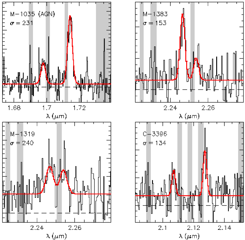
Figure 2: Gaussian fits to emission lines. For M–1035 and C–3396 the lines are [O iii] 4959,5007 Å; for M–1383 and M–1319 they are H$\alpha$ and [N ii] $\lambda 6584$. Raw spectra are shown in black; red lines are best fitting models. Line widths are also shown, corrected for instrumental broadening. The line widths are substantial, typical of massive nearby galaxies.

Figure 3: Spectral energy distributions of $J_{s}-K_{s}$ selected galaxies with spectroscopic redshifts $z>2$. Large open circles show observed fluxes, and solid circles show fluxes corrected for emission line contributions. Thin lines show best fitting stellar population synthesis models with constant star formation rate and varying age and dust content. Small open circles are model fluxes in the broad band filters. The median age is 1.6 Gyr and the median absorption $A_{V}=1.8$ mag. For comparison the lower right panel shows the median best fitting model to $z=3$ Lyman break galaxies from Shapley et al. (2001), with a much younger age of 0.3 Gyr and absorption $A_{V}=0.5$ mag.

M–1035 – This object was identified as a Type-II AGN based on its narrow Ly$\alpha$, C iv and He ii lines in the rest-frame UV (van Dokkum et al. 2003). We observed the galaxy in the N-4, N-5 ($H$), and N-7 ($K$) bands. The continuum was detected in every band as well as several emission lines. All lines have widths $<2000$ km s^-1, confirming the Type-II classification (see, e.g., Stern et al. 2002; Norman et al. 2002). The [O iii] lines have width $\sigma=231$ km s^-1 (see § 4.2.3), and the broadest feature is the H$\alpha$ + [N ii] complex, width a combined FWHM of 1600 km s^-1. The object is a faint hard X-ray source (Johnson, Best, & Almaini 2003), consistent with the idea that the central engine is (partially) obscured by dust.

M–1356 – The rest-frame UV spectrum of M–1356 indicates the presence of an AGN (van Dokkum et al. 2003), with characteristics of Broad Absorption Line QSOs. The UV spectrum shows strong Nitrogen lines indicating a high metallicity. The $K$-band spectrum shows fairly broad H$\alpha$ + [N ii] emission with FWHM $\sim 2500$ km s^-1. This galaxy is not a Chandra source, consistent with the BAL nature of its active nucleus (e.g., Green & Mathur 1996). We note that due to a revision of our photometry since the NIRSPEC observations this galaxy has $J_{s}-K_{s}=2.13$, and hence falls blueward of our DRG criterion; removing this galaxy from the analysis does not alter the conclusions in any way.

M–1383 – For galaxy M–1383 the rest-frame optical spectroscopy implies a revision of the rest-frame UV redshift. We deduced a redshift $z=3.525$ from faint absorption lines in the rest-frame UV (van Dokkum et al. 2003); however, in the $K$-band we detect H$\alpha$ and [N ii] redshifted to $z=2.423$, making this the fourth red galaxy at $z\approx 2.43$ in the MS 1054–03 field. The revised redshift is consistent with the photometric redshift in van Dokkum et al. (2003). The rest-UV spectrum has low S/N, and the previously published redshift may simply be in error. Another possibility is that the blue feature seen off-center in this object is a background galaxy at $z=3.52$.

MS–1319 – The brightest galaxy in the sample in the $K$-band, enabling the direct detection of the continuum break responsible for its red $J_{s}-K_{s}$ color (§ 4.1). The $K$-band spectrum shows H$\alpha$ and [N ii].

C–237 – The spectrum of C–237 shows a broad, low S/N H$\alpha$ + [N ii] complex. Higher S/N spectra are needed to measure the width reliably, but we infer that the galaxy probably hosts an active nucleus. The association of C–237 with a hard X-ray source (Alexander et al. 2003) is consistent with this interpretation.

C–3396 – The redshifted [O iii] lines are detected at the expected locations; H$\beta$ is barely detected. The lines are resolved in the spatial direction, and there is some evidence for a velocity gradient. The galaxy is a faint soft source in the 1 Ms Chandra catalog (Giacconi et al. 2002), possibly indicating a very strong star burst. The X-ray properties of DRGs will be discussed in K. Rubin et al., in preparation.

4.2.2 Line Luminosities and Equivalent Widths

For each galaxy we modeled the continuum with a second order polynomial, fitted to the binned spectrum. Emission lines were masked in the fit. After subtracting the continuum, line fluxes were measured by summing the counts in the residual spectrum in regions centered on the redshifted lines. The width of these regions was typically 50 Å, except for two cases where H$\alpha$ is broader (see § 4.2.1). Errors were derived from simulations, by placing random apertures in regions with similar noise characteristics and by varying the parameters of the continuum fit.

Calibration of the line fluxes was performed in the following way. First the emission lines were added to the continuum fits; we used the fits rather than the measured continuum to limit the effects of sky line residuals. Next, the spectra were converted from $F_{\lambda}$ to $F_{\nu}$ and convolved with the VLT ISAAC broad band filter response curves appropriate for the observed wavelength range. Finally, the spectra were normalized using the measured magnitudes in these filters. The broad band photometry is accurate to $\approx 0.05$ mag. Total magnitudes were used, so that the measured line fluxes are effectively corrected to an aperture covering the entire galaxy. Equivalent widths were determined directly by comparing the line flux to the continuum fit at the location of the line, and require no absolute calibration. The measured line properties are listed in Table 2.

4.2.3 Line Widths

We determined line widths by fitting Gaussian models to the 1D spectra. Galaxies C–237 and M–1356 were excluded, as for both galaxies the H$\alpha$ + [Nii] line complex is too broad to separate the two lines with confidence. Galaxy M–1035 also has a broad H$\alpha$ line complex, but for this object we can obtain a reliable line width from its [O iii] lines.

For each of the four galaxies two lines were detected (see Table 2); both lines were fitted simultaneously. Free parameters in the fits are the redshift, fluxes of both lines, and the line width. The continuum was allowed to vary within the uncertainties of the polynomical fit to the binned spectrum (see § 4.2.2). The fitting procedure minimizes the sum of the absolute differences between model and data to limit the effects of outliers; minimizing the rms gives similar results. Pixels in regions of strong sky lines were excluded from the fit.

Best fitting models are shown in Fig. 2; line widths corrected for instrumental broadening are listed in Table 2. Errors were determined from fits to simulated spectra. One-dimensional noise spectra were extracted from the 2D spectra at random spatial positions and added to model spectra; these artifical spectra have very similar noise characteristics as the galaxy spectra. The errors were determined from the biweight width of the distribution of differences between true and measured line widths. The line width of galaxy C–3396 has a large (asymmetric) uncertainty; although the faint [O iii] lines are resolved, their width is not well determined.

5 Stellar Populations

5.1 Fits to Broad Band Photometry

For all galaxies high quality photometry is available over the wavelength range $0.35-2.2\,\mu$, and following previous studies of LBGs we fit model SEDs to the photometric data to constrain star formation rates, ages, and the extinction of the stellar continua. For completeness we include galaxy M–140 in this analysis, as it is the only DRG with redshift that was not observed with NIRSPEC, and its redshift implies that the NIR photometry will only be marginally affected by emission lines. We note that similar fits were presented in van Dokkum et al. (2003) for the five galaxies in the MS 1054–03 field. Fits to the entire sample of DRGs in MS 1054–03 (i.e., including those without spectroscopic redshift) are presented in Förster Schreiber et al. (2004).

5.1.1 Corrections for Emission Lines

Strong emission lines can affect the broad band fluxes of high redshift galaxies and may cause systematic errors in derived stellar population parameters. In Lyman break galaxies emission lines typically contribute $\sim 15$ % to the broad band fluxes (Shapley et al. 2001). This estimate is somewhat uncertain because it relies on absolute calibration of the NIR spectroscopy (see Pettini et al. 2001). The corrections can be determined with greater confidence for the present sample of DRGs because the continuum is detected in every case.

Figure 4: Results of Bruzual & Charlot (2003) model fits to the emission-line corrected broad-band SEDs. Large symbols show the best fitting values of age and star formation rate. Small symbols show the range in best fit parameters for each galaxy, derived from randomizing the photometry within the (random and systematic) photometric errors. Dashed lines are of constant mass. The ages and star formation rates have substantial uncertainties, but the stellar masses are well constrained. They are very high at $1-5\,\times\,10^{11}\,M_{\odot}$.

Emission line corrections for all observed photometric bands are listed in Table 3. Values in parentheses have been calculated with the help of the following relations, determined from the Jansen et al. (2000) sample of nearby galaxies:

$$W_{\lambda}({\rm[O}\,{\rm II}{\rm]})=0.98\pm 0.52\,\times\,W_{\lambda}({\rm H}\alpha)$$ (1)

$$W_{\lambda}({\rm H}\beta+{\rm[O}\,{\rm III}{\rm]})=0.53\pm 0.22\,\times\,W_{\lambda}({\rm H}\alpha)$$ (2)

$$W_{\lambda}({\rm[O}\,{\rm II}{\rm]})=1.8\pm 0.4\,\times\,W_{\lambda}(\lambda 5007).$$ (3)

The corrections range from $<0.05$ to $0.16$ magnitudes in the $K_{s}$ band, with a median of $0.08$. Our sample is biased toward the presence of emission lines in the rest frame UV (as this makes it easier to measure the redshift), and it is reasonable to assume that it is also biased toward the presence of lines in the rest frame optical. Therefore, the small contributions measured here strongly suggest that the red colors of $J_{s}-K_{s}$ selected galaxies in general are caused by red continua rather than the presence of strong emission lines in the $K_{s}$ band.

5.1.2 Fitting Methodology and Results

Emission-line corrected SEDs are shown in Fig. 3 (solid symbols), along with the uncorrected photometry (open symbols). We fitted stellar population synthesis models to the corrected photometry. The Bruzual & Charlot (2003) models were used; this latest version is based on a new library of stellar spectra and has updated prescriptions for AGB stars.

A major systematic uncertainty in this type of analysis is the parameterization of the star formation history (Shapley et al. 2001; Papovich et al. 2001). The ubiquitous emission line detections in our sample imply that the galaxies are not evolving passively, and that models in which all stars were formed in a single burst at high redshift are not appropriate. For simplicity we limit the discussion to models with constant star formation rates, characterized by three parameters: the time since the onset of star formation (the age), the star formation rate, and the extinction. Models with a declining star formation rate are discussed briefly in § 5.3, and in Förster Schreiber et al. (2004). We only consider solar metallicity models; as we show in § 5.6 such models are consistent with the limited information we have on the abundances of DRGs.

The publicly available hyperz photometric redshift code (Bolzonella, Miralles, & Pelló 2000) was used for the fitting. Its template library was updated with the Bruzual & Charlot (2003) models and the redshift was held fixed at the spectroscopic value. The Calzetti et al. (2000) reddening law was applied; we tested that the results are not very sensitive to the assumed extinction curve. A minimum photometric error of 0.05 was assumed, so that individual data points with very small formal errors do not dominate the $\chi^{2}$ minimalization.

Best fitting SEDs are overplotted in Fig. 3. Corresponding star formation rates, ages and reddening values are listed in Table 4. The constant star formation models provide reasonable descriptions of the photometric data. The median absolute difference between data and model is $\approx 0.07$ mag for galaxies C–3396, M–140, M–1356 and M–1383, and $\approx 0.2$ mag for the other three galaxies. However, as the errors in the photometry are typically much smaller, the $\chi^{2}$ minima are mostly greater than one, with median 2.9.

Confidence limits on the derived parameters were determined in the following way. For each galaxy, 500 simulated SED datapoints were created by randomizing the photometry within the uncertainties. In order to account for systematic errors and template mismatch the uncertainties were multiplied by the square root of the $\chi^{2}$ value of the best fitting model. The simulated SEDs were modeled using the same procedure as the observed SEDs. Figure 4 shows the best fit age and star formation rate for each galaxy (large symbols) along with values for 100 of the simulated SEDs (small symbols). Uncertainties in the ages are highly correlated with those in the star formation rates. As stellar mass is the product of star formation and age in these models the uncertainty in this parameter is relatively small.

The $1\sigma$ confidence limits listed in Table 4 were determined from the simulations by calculating the widths of the distributions of age, star formation rate, reddening, and stellar mass. The confidence limits are generally not symmetric. For all galaxies “maximally old” fits fall within the confidence limits, i.e., in every case the upper limit to the age is set by the age of the universe at the epoch of observation. The uncertainties are largest for galaxy M–1383, which has a smooth SED without a pronounced break.

The stellar populations in these galaxies appear to be quite similar. All seven have relatively old ages ranging from 0.7 – 2.6 Gyr, and substantial extinction ranging from 0.9 – 2.3 magnitudes in the rest frame $V$ band. The implied star formation rates range from 102 $M_{\odot}$ yr^-1 to 468 $M_{\odot}$ yr^-1, and the stellar masses from $1.3\times 10^{11}\,M_{\odot}$ to $4.9\times 10^{11}\,M_{\odot}$. We note that the parameters for galaxies M–1035 and M–1356 are uncertain, as their active nuclei may affect their continua.

5.2 Constraints from H$\alpha$

The SED fitting results suggest that the DRGs are unlike Lyman break galaxies: their star formation rates are similar, but their ages and dust content are substantially larger. The implied stellar masses rival those of elliptical galaxies in the nearby Universe. In light of these important implications and the systematic uncertainties associated with SED fitting it is critical to compare the results to those implied by our NIR spectroscopy.

5.2.1 Star Formation Rates and Ages

The H$\alpha$ emission line measures the current star formation rate (through the line luminosity) as well as the ratio of current and past star formation (through the equivalent width). Dust-corrected line luminosities can be converted to the instantaneous star formation rate using

$${\rm SFR}\,(M_{\odot}\,{\rm yr}^{-1})=7.9\times 10^{-42}L_{{\rm H}\alpha}({\rm ergs\,s}^{-1})$$ (4)

(Kennicutt 1998). In local galaxies this relation is consistent with other indicators of the star formation rate, such as radio luminosity and far-infrared luminosity (e.g., Kewley et al. 2002). Such studies have not yet been done systematically at high redshift, although results for LBGs suggest that this correspondence holds for these galaxies as well (e.g., Reddy & Steidel 2004).

For constant star formation histories the equivalent width has a one-to-one relation with the time elapsed since the onset of star formation (the age). The dependence of age on equivalent width has the form of a powerlaw. Using the Bruzual & Charlot (2003) models to find the continuum luminosity and Eq. 4 to convert line luminosity to star formation rate we find

$$\log{\rm(age)}=13.2-2.4\,\log\,W_{\lambda}({\rm H}\alpha)$$ (5)

with $W_{\lambda}$ the rest frame equivalent width in Å and the age in years. Over the range $7.5<\log{\rm(age)}<9.5$ the powerlaw approximation holds to a few percent. Note that the relation depends on the conversion factor between star formation rate and line luminosity (Eq. 4), but not on the star formation rate itself.

The main uncertainty is attenuation by dust. H$\alpha$ luminosities are usually corrected for extinction by comparing them to H$\beta$, assuming the intrinsic ratio of case-B recombination. However, as we have not measured the H$\alpha$/H$\beta$ pair in any of the galaxies, we have to derive the extinction from the attenuation of the stellar continuum. Studies of nearby and distant galaxies indicate that the extinction toward Hii regions is at least as high as that of the stellar continuum (e.g., Kennicutt, 1992, 1998; Calzetti et al. 1996; Erb et al. 2003). The relation depends on the distribution of the dust, which is difficult to constrain observationally. In the following, we consider two cases: 1) no additional extinction toward Hii regions. In this case, $L({\rm H}\alpha)_{\rm corr}=10^{0.37\,A_{V}}L({\rm H}\alpha)_{\rm obs}$ (with $A_{V}$ the extinction of the stellar continuum), and $W_{\lambda}({\rm H}\alpha)_{\rm corr}=W_{\lambda}({\rm H}\alpha)_{\rm obs}$; and 2) additional $V$-band extinction of one magnitude. In that case, $L({\rm H}\alpha)_{\rm corr}=10^{0.37\,(A_{V}+1)}L({\rm H}\alpha)_{\rm obs}$, and $W_{\lambda}({\rm H}\alpha)_{\rm corr}=2.34W_{\lambda}({\rm H}\alpha)_{\rm obs}$. These two cases probably bracket the actual values.

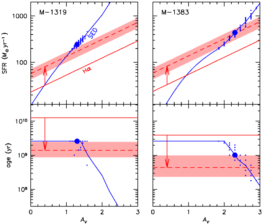
Figure 5: Combined constraints on stellar population parameters from SED fitting (blue) and H$\alpha$ luminosity and equivalent width (red). The H$\alpha$ constraints depend on the assumed extinction toward H ii regions: the solid line assumes that it is equal to the extinction of the stellar continuum, and the dashed line assumes an additional extinction of one magnitude. The bands indicate 1$\sigma$ observational errors in the H$\alpha$ measurements. Note that the SED constraints on the ages are bounded by the age of the Universe at the epoch of observation. Small dots are derived from error simulations (see Fig. 4). The H$\alpha$ constraints are less sensitive to $A_{V}$ than the SED constraints, and consistent solutions are obtained where the red and blue lines intersect. The regions where the curves intersect coincide with the $\chi^{2}$ minima of the SED fits, for $A_{V,{\rm H}\,{II}}=A_{V,{\rm SED}}+1$.

5.2.2 Consistency with SED fits

We first consider whether the ages, star formation rates, and extinction derived from the SED fits are consistent with the observed luminosities and equivalent widths of H$\alpha$. Values implied by the SED fits were calculated using Eqs. 4 and 5, and the star formation rates and ages listed in Table 4. Extinction corrections were applied following the procedure outlined above.

Comparison of observed H$\alpha$ line luminosities (a) and equivalent widths (b) to predicted values from the SED modeling. Luminosity predictions were computed from the star formation rates; equivalent widths from the ages. Open symbols assume that the extinction toward Hii regions is equal to that of the stellar continuum; solid symbols assume one magnitude additional extinction. The H$\alpha$ measurements are in good agreement with the predictions from the SED modeling.

In Fig. 5.2.2(a) the line luminosities implied by the SED fits are compared to the observed ones. Galaxies M–1035 and M–1356 are not shown, as their emission lines are almost certainly dominated by their active nuclei. For C–3396 we use $L_{{\rm H}\alpha}=2.75L_{{\rm H}\beta}$ (Osterbrock 1989), after taking differential extinction into account. The SED results overpredict the H$\alpha$ observations for $A_{V,\,\rm{H\,II}}=A_{V,\,{\rm SED}}$, but they agree very well if Hii regions suffer additional extinction of approximately one magnitude.

In Fig. 5.2.2(b) predicted equivalent widths are compared to the observed ones. The value for C–3396 was determined using $W_{\lambda}({\rm H}\beta)=0.22W_{\lambda}({\rm H}\alpha)$ (Jansen et al. 2000). Again, the data are in good agreement and indicate additional extinction of one magnitude toward Hii regions.

5.2.3 Constraints on $A_{V}$

Although the agreement between SED fits and H$\alpha$ measurements is encouraging the two constraints are not truly independent, as they both rely on the extinction as derived from the broad band photometry. Furthermore, the additional extinction toward Hii regions is a free parameter in the modeling. Here we discuss the dependence of the age and star formation rate on the dust content in more detail. We only consider the two non-active galaxies for which H$\alpha$ has been reliably measured (M–1383 and M–1319).

We first determine the dependence of the SED fitting results on the extinction. Rather than having $A_{V}$ as a free parameter in the fits it was held fixed at values ranging from $A_{V}=0$ to $A_{V}=3$; only the age and star formation rate were allowed to vary. As shown in Figure 5 (blue lines) the dependencies are quite strong, because the age and star formation rate are very sensitive to the UV flux, which is a strong function of $A_{V}$.

Next we examine the extinction-dependence of the constraints derived from H$\alpha$ (red lines). The solid lines show the derived star formation rates and ages assuming $A_{V,\,{\rm H\,II}}=A_{V,\,{\rm SED}}$. Importantly, the implied ages are higher than the age of the Universe at $z=2.43$ with this assumption, in particular for galaxy M–1319. The low H$\alpha$ equivalent widths thus imply either additional absorption toward Hii regions, or a declining star formation rate (see § 5.3). Note that this result follows directly from Eq. 5, and is independent from the SED fits. Dashed lines show the effect of an additional magnitude of extinction for the line emitting gas; with this assumption the implied ages are lower than the age of the Universe.

Furthermore, the dependencies are much weaker than for the SED fits, because they are determined by the absorption at $6563$ Å rather than in the UV. As an example, for galaxy M–1383 the H$\alpha$-derived star formation rate varies from $25\,M_{\odot}\,$yr^-1 to $300\,M_{\odot}\,$yr^-1 for $A_{V}=0-3$, whereas the star formation rate derived from the SED fits varies between zero and $2000\,M_{\odot}\,$yr^-1. The different dependencies on the extinction can be utilized: we can determine $A_{V}$ by requiring that the ages and star formation rates derived from the SED fits are equal to those derived from H$\alpha$. Consistent solutions are obtained at the intersections of the lines derived from the SED fits and those derived from H$\alpha$. We find $0.8\lesssim A_{V}\lesssim 1.2$ for M–1319 and $1.8\lesssim A_{V}\lesssim 2.6$ for M–1383, if the additional extinction toward Hii regions is approximately one magnitude.

This derivation of the extinction is independent of the values corresponding to the best fitting SED: there is no “built-in” requirement that the solutions with the lowest $\chi^{2}$ residual should fall in the regions of the plots where the SED constraints and the H$\alpha$ constraints are consistent with each other. Nevertheless, they do: the large solid symbols correspond to the best fitting SEDs (shown in Fig. 3); as in Fig. 4 small dots indicate the uncertainty. These results considerably strengthen the conclusion from § 5.2.2: the constraints on ages and star formation rates from H$\alpha$ are consistent with those derived from the broad band photometry only for the values of $A_{V}$ corresponding to the best fitting SEDs. Furthermore, the additional extinction toward Hii regions (which was treated as a free parameter in § 5.2.2) is required by the strict upper limit on the ages imposed by the age of the Universe at $z=2.43$.

5.3 Models with Declining Star Formation Rates

The inferred star formation rates are very sensitive to the (high) extinction that we derive. We can determine the “minimum” star formation rates for galaxies M–1319 and M–1383 by applying no extinction correction to their H$\alpha$ luminosities. The uncorrected star formation rates are 23 $M_{\odot}$ yr^-1 and 24 $M_{\odot}$ yr^-1 respectively, i.e., an order of magnitude lower than the extinction-corrected values (see Table 5). As we demonstrated in the preceeding Sections, the SEDs of the galaxies, and the H$\alpha$ equivalent widths, cannot be fitted with continuous star formation models with low extinction. Here we investigate what values we find for the extinction and star formation rates if we allow for the possibility that the star formation rates are not constant but declining. We only consider the two non-active galaxies with measured H$\alpha$ luminosities; a more extensive discussion is given in Förster Schreiber et al. (2004), which describes SED fits to the full sample of galaxies with $K_{s}<21.7$ and $J_{s}-K_{s}>2.3$ in the MS 1054–03 field.

Galaxies M–1319 and M–1383 were fitted with Bruzual & Charlot (2003) models characterized by a star formation history with an e-folding time $\tau=300$ Myr. Both galaxies are well fitted by this model; differences in the best fitting $\chi^{2}$ between the declining and the continuous model are not statistically significant. For both galaxies the $\tau$-model gives lower dust content, lower ages, and lower star formation rates than the continuous model; values are listed in Table 5. However, the mean star formation rate over the lifetime of the galaxy is actually slightly higher in the $\tau$-model: $507\,M_{\odot}$ yr^-1 for M–1383 and $330\,M_{\odot}$ yr^-1 for M–1319. As a result, the stellar masses in the two models are similar. These effects are illustrated in Fig. 5.3, which shows the star formation histories of both galaxies for both models. The effect of the $\tau$-model is to make the star formation history more concentrated and peaked in time, but it does not substantially change the total number of stars formed.

We conclude that the extinction and star formation rates are model-dependent, and can be lower by factors of $2-3$ if the star formation histories are modified. However, the stellar masses are robust, because declining models have a much higher star formation rate at earlier epochs (see Fig. 5.3).

Best fitting star formation histories of galaxies M–1383 (red) and M–1319 (blue), for a continuous star formation model (dashed) and a $\tau$-model with an e-folding time of 0.3 Gyr (solid). Models with declining star formation rates produce lower star formation rates at the epoch of observation, but they have much higher star formation rates at earlier epochs.

5.4 Continuum Break

For one galaxy (M–1319) we obtained a spectrum in the rest-frame wavelength range 3750 Å – 4550 Å (see § 4.1), providing an additional constraint on its stellar population. The spectrum can be used to disentangle the effects of age and dust. Young dusty galaxies have smooth SEDs, whereas galaxies with stellar populations older than $\sim 500$ Myr have a pronounced discontinuity at $\lambda 3625$ Å (the Balmer discontinuity) or $\lambda 4000$ Å (the Ca ii H+K break).

The spectrum is of insufficient quality to constrain the age and dust content independently. Instead, we generated model spectra for different values of $A_{V}$ by fitting constant star formation models to the broad band photometry (see § 5.2.3). This constrained fit ensures that the best fitting model is consistent with the broad band photometry (or at least as close as possible for that particular value of $A_{V}$). The models were binned in the same way as the observed spectrum, and fitted using a $\chi^{2}$ minimalization.

The best fitting $A_{V}=0.6^{+1.2}_{-0.6}$, consistent with the extinction derived from the broad band photometry ($A_{V}=1.3\pm 0.1$) and from the comparison of SED fits and H$\alpha$ constraints ($A_{V}=0.8-1.2$). The uncertainties are quite large, partly because the spectrum does not extend blueward of the Balmer break. Models with extinction higher than $A_{V}\approx 2$ fit poorly because they overpredict the flux blueward of 3900 Å and underpredict the flux redward of 4400 Å; an example with $A_{V}=3$ is shown by the red histogram in Fig. 4.1. The best fit to the broad band photometry is shown in blue; this model is a good match to the observed spectrum.

5.5 SCUBA Detection

Independent constraints on the star formation rate are very important as they can help break the degeneracy between the form of the star formation history and the current star formation rate (see § 5.3). K. Knudsen et al. (in preparation) obtained a deep, large area SCUBA map of the MS 1054–03 field, and we have performed an initial investigation of coincidences of SCUBA detections and $J_{s}-K_{s}$ selected galaxies. Interestingly galaxy M–1383, the object in our sample with the highest inferred dust content, is very likely a SCUBA source.

The object is detected with an 850 $\mu$ flux density of $5.1\pm 1.5$ mJy. Assuming the infrared SED is similar to that of Arp 220 the IR luminosity is $5\times 10^{12}\,L_{\odot}$, and the implied star formation rate is $\sim 500\,M_{\odot}$ yr^-1, in excellent agreement with the (extinction-corrected) value of $\sim 400\,M_{\odot}$ yr^-1 that we determine from the stellar SED and H$\alpha$ in the constant star formation model (see Table 5). We note that such a good agreement is uncharacteristic of local ultra-luminous infrared galaxies, as star forming regions in these galaxies usually suffer from such high visual extinction that it is very difficult or impossible to correct for it. A full analysis of submm and X-ray constraints on the star formation rates of DRGs will be presented elsewhere; here we note that the submm data for this galaxy provide strong independent support for our modeling procedures.

5.6 Metallicities

Determining metallicities for high redshift galaxies is difficult, as generally only a limited number of (bright) emission lines is available. The most widely used metallicity indicator for faint galaxies is the $R_{23}$ index, which relates O/H to the relative intensities of [O ii] $\lambda 3727$, [O iii] $\lambda\lambda 4959,5007$, and H$\beta$ (Pagel et al. 1979; Kobulnicky, Kennicutt, & Pizagno 1999). Using this indicator Pettini et al. (2001) derive abundances for five LBGs of between $0.1\times$ and $1\times$ Solar, with the main uncertainty the double-valued nature of the $R_{23}$ index.

We do not have the required measurements to calculate the $R_{23}$ index for any of the four non-active galaxies in our sample. However, for two objects the luminosities of H$\alpha$ and [N ii] $\lambda 6584$ are available, enabling us to derive metallicities using the “N2” index. This indicator is defined as N2$=\log$ ([N ii]  $\lambda 6584/$ H$\alpha$); it was first suggested by Storchi-Bergmann, Calzetti, & Kinney (1994) and discussed recently by Denicoló, Terlevich, & Terlevich (2002). Advantages of the N2 indicator are that it has a single-valued dependence on the oxygen abundance and that it is insensitive to reddening. However, it is sensitive to ionization and, as oxygen is not measured directly, to O/N variations (see, e.g., Denicoló et al. 2002).

For objects M–1383 and M–1319 we find ${\rm N}2=-0.40\pm 0.16$ and ${\rm N}2=-0.10\pm 0.13$ respectively. Using the calibration of Denicoló et al. (2002),

$$12+\log({\rm O/H})=9.12(\pm 0.05)+0.73(\pm 0.10)\times{\rm N2},$$ (6)

we find $12+\log({\rm O/H})=8.8\pm 0.3$ and $9.0\pm 0.3$ respectively (where we used an intrinsic scatter in the method of 0.2 dex; see Denicoló et al. 2002). As the Solar abundance $12+\log({\rm O/H})_{\odot}=8.83$, we infer that the abundances of the two $J_{s}-K_{s}$ selected galaxies are $1\times$ and $1.5\times$ Solar, with uncertainties of a factor of two. We conclude that current evidence suggests that red $z>2$ galaxies are already quite metal rich, as might have been expected from their high dust content and extended star formation histories.

6 Kinematics

6.1 Masses and $M/L$ Ratios

The stellar masses implied by the SED fits are substantial, ranging from $1.3-4.9\times 10^{11}\,M_{\odot}$, with median $3.5\times 10^{11}\,M_{\odot}$. Although these results are supported by the H$\alpha$ luminosities and equivalent widths significant systematic uncertainties remain: the SED fitting is dependent on the assumed IMF and metallicity, and both methods are sensitive to the assumed star formation history and extinction law.

Independent constraints on the masses of the red galaxies can be obtained from their kinematics. Line widths were measured for four galaxies, one of which harbors an AGN (see § 4.2.3). The widths are substantial, and range from 134 km s^-1 to 240 km s^-1. The line broadening can be caused by regular rotation in a disk, random motions, or non-gravitational effects. Rix et al. (1997) derive an empirically motivated transformation from observed line width to rotation velocity in a disk; applying their relation $\sigma\approx 0.6V_{c}$ gives rotation velocities in the range 200–400 km s^-1. The kinematics are thus in qualitative agreement with the high masses inferred for the stars.

The large linewidths imply that the four red galaxies are very massive, unless they are highly compact. The galaxies are faint in the rest-frame UV which makes it difficult to measure their sizes from optical HST images. Fig. 6.1 shows $K_{s}$ images of the four galaxies with measured velocity dispersions, all taken with ISAAC on the VLT in $\approx 0\farcs 5$ seeing. All four galaxies are resolved in these ground-based images. Effective radii are $\sim 0\farcs 5$, with the largest galaxy (M–1383) having $r_{e}\approx 0\farcs 7$ (Trujillo et al. 2004 and in preparation). Using $r_{e}\approx 0\farcs 5$ as a reasonable estimate for the size, the median $\sigma\approx 200$ km s^-1 for the velocity dispersion, and the same normalization as Pettini et al. (2001), we find $M_{\rm dyn}\sim 2\times 10^{11}\,M_{\odot}$. This number is in good agreement with the stellar mass estimates.

Ground based $K_{s}$ images of the four galaxies with measured line widths, obtained with ISAAC on the VLT. Images are $5^{\prime\prime}\times 5^{\prime\prime}$; the FWHM image quality is $\approx 0\farcs 5$. All four galaxies are resolved; they have typical effective radii of $\sim 0\farcs 5$.

Figure 6: Correlations of rest-frame optical linewidth with rest-frame $V$-band absolute magnitude (a), rest-frame $U-V$ color (b), and stellar mass (c). Small open circles are Lyman-break galaxies at $z\approx 3$, the large open symbol is a LBG at $z=2.19$, and filled circles are $J_{s}-K_{s}$ selected galaxies with mean $z=2.6$. Linewidth correlates with luminosity, color, and stellar mass in the combined sample. The line in (c) is the relation between rotation velocity and baryonic mass determined for local galaxies by McGaugh et al. (2002), using $\sigma\approx 0.6V_{c}$ (Rix et al. 1997). This relation provides an excellent fit to the $z>2$ galaxies.

The median absolute $V$ magnitude of the four galaxies is $-23.6$ (see below). With $M\sim 2\times 10^{11}\,M_{\odot}$ this implies dynamical mass-to-light ratios $M/L_{V}\sim 0.8$ in Solar units, a factor of $\sim 5$ higher than $z\approx 3$ Lyman-break galaxies (Pettini et al. 2001). Based on the range of values within our sample we estimate that the uncertainty in this number is approximately a factor of two.

6.2 Correlations with Linewidth

Pettini et al. (2001) studied Tully-Fisher (Tully & Fisher 1977) like correlations for LBGs, by comparing their kinematics (as measured by the line width of rest-frame optical emission lines) to their rest-frame UV and optical magnitudes. No correlations were found over the range $50$ km s^-1 $\leq\sigma\leq$ 115 km s^-1. Here we add the four red $z>2$ galaxies with measured linewidths to Pettini’s sample and re-assess the existence of correlations with linewidth at $z\sim 3$.

Rest-frame $V$ magnitudes were determined from observed $K_{s}$ magnitudes and $J_{s}-K_{s}$ colors. For each galaxy we derive a transformation between observed magnitudes and rest-frame magnitudes of the form

$$V_{\rm rest}=K_{s}+\alpha(J_{s}-K_{s})+\beta.$$ (7)

The constants $\alpha$ and $\beta$ depend on the redshift, but only weakly on the spectral energy distribution of the galaxy (see van Dokkum & Franx 1996). Using spectral energy distributions from Bolzonella et al. (2000) we determined that, for $z\sim 3$, the transformations have the same form within $\sim 5$ % for SEDs ranging from starburst to early-type. Shapley et al. (2001) give $K_{s}$-band magnitudes for nine galaxies in the Pettini et al. (2001) sample, and $J-K_{s}$ colors for six. For the three LBGs that have not been observed in $J$ we use synthetic $J-K_{s}$ colors; the added uncertainty in $V_{\rm rest}$ is negligible as $\alpha=-0.01$ for $z=3$.

Figure 6(a) shows the “Tully-Fisher” diagram of rest-frame optical linewidth (corrected for instrumental resolution) versus rest-frame absolute $V$ magnitude, for $z>2$ galaxies. The four $J_{s}-K_{s}$ selected galaxies have higher linewidths and are on average more luminous than $z\approx 3$ LBGs. Although visually suggestive, the Spearman rank and Pearson correlation tests give probabilities of $\sim 50$ % that $\log\sigma$ and $M_{V}$ are uncorrelated, and we conclude the evidence for the existence of a luminosity-linewidth relation at $z\sim 3$ is not yet conclusive. Erb et al. (2003) find that $z\approx 2$ LBGs have on average higher linewidths than those that have been observed by Pettini et al. (2001) at $z\approx 3$, and it will be interesting to see where these galaxies lie on the Tully-Fisher diagram. The only $z\approx 2$ LBG from Erb et al. (2003) with measured $K$ magnitude (Q1700-BX691 at $z=2.19$) is indicated with a large open symbol in Fig. 6(a).

In Fig. 6(b) linewidth is plotted versus rest-frame $U-V$ color, which were derived from the observed $J_{s}-K_{s}$ colors in a similar way as the rest-frame $V$ magnitudes. Only the six Lyman-break galaxies with measured $J-K_{s}$ colors are included. There is a striking correlation, with significance $>97$ %. The figure also clearly demonstrates the large difference in rest-frame colors between LBGs and $J_{s}-K_{s}$ selected galaxies. In the local universe similar trends exist, with more massive galaxies generally being redder.

Finally, Fig. 6(c) shows the relation between linewidth and stellar mass. To limit systematic effects we determined the stellar masses of the LBGs with our own methods, using the photometry presented in Shapley et al. (2001) and Steidel et al. (2003). The median stellar mass is $2\times 10^{10}\,M_{\odot}$, very similar to what Shapley et al. (2001) finds for the same nine objects. The correlation has a significance of $\approx 90$ %. The line shows the “baryonic Tully-Fisher relation” of McGaugh et al. (2000), which is an empirical relation between rotation velocity and total mass in stars and gas (for galaxies with $M_{*}>10^{9}\,M_{\odot}$ this is approximately equal to the stellar mass alone). With $\sigma\approx 0.6V_{c}$ this relation takes the form $M_{*}=312\,\sigma^{4}\,M_{\odot}$ in our cosmology; without any further scaling it provides a remarkably good fit to the $z>2$ data.

Figure 7: Correlations of H$\alpha$ equivalent width (a,b) and the [N ii]  $\lambda 6584/$ H$\alpha$ ratio (c,d) with rest-frame $U-V$ color and $V$-band absolute magnitude, for samples of star-forming galaxies. Shown are nearby normal galaxies from the Nearby Field Galaxy Survey (Jansen et al. 2000,2001) (small dots), nearby Luminous InfraRed Galaxies from Arhus et al. (1989) (crosses), LBGs from Pettini et al. (2001) (open circles), and the three non-active DRGs with measured Balmer lines from the present study (large solid circles). The metallicity scale on the right axis of (c) and (d) corresponds to the LBGs from Pettini et al. (2001). This scale is coupled to the [N ii] / H$\alpha$ scale through the Denicolo et al. (2002) calibration. No extinction corrections were made. The broken line in (b) indicates a line of constant H$\alpha$ luminosity; the dashed line in (c) and (d) indicates Solar metallicity. Contrary to LBGs, the red $z>2$ galaxies have similar colors, metallicities, and H$\alpha$ equivalent widhts as normal nearby galaxies.

We note that the analysis may be affected by selection effects, as we combine very different samples of galaxies in Fig. 6. Pettini’s LBGs are at slightly higher mean redshift than the DRGs, and their linewidths were measured from the [O iii] lines instead of H$\alpha$. The $z\approx 2$ LBG sample of Erb et al. (2003) shows a much larger range in linewidth than Pettini’s $z\approx 3$ sample. This may be caused by differences in selection (the Pettini sample was selected to be very bright in the rest-frame UV, which may select relatively low mass objects; see Erb et al. 2003), but may also hint at systematic differences between linewidths determined from H$\alpha$ and the oxygen lines, or even evolution. It will be interesting to see where the Erb et al. objects fall in the panels of Fig. 6, especially those with the highest linewidths.

We are also limited by small number statistics. In particular, the reason why linewidth appears to correlate most strongly with color may simply be that there is no $J$-band measurement given by Shapley et al. (2001) for West MMD11, which is a luminous and apparently massive Scuba source with very small linewidth ($\sigma=53\pm 5$ km s^-1). When this object is arbitrarily removed in Figs. 6(a) and (c) as well the correlation significance jumps to $\approx 98$ % in both cases.

6.3 Outflows

A major result of kinematic studies of LBGs is that they exhibit galactic-scale outflows (Franx et al. 1997; Pettini et al. 1998, 2000; Adelberger et al. 2003). The main evidence comes from comparisons of the radial velocities of Ly$\alpha$, UV absorption lines, and rest-frame optical emission lines. The UV absorption lines are blueshifted with respect to the optical lines as they trace the gas flowing towards us, whereas Ly$\alpha$ emission appears redshifted as it originates from the back of the shell of outflowing material (see, e.g., Pettini et al. 2001 for details). In LBGs winds have typical velocities of $\sim 300$ km s^-1 (with a large range), and are thought to play an important role in enriching their surrounding medium (Adelberger et al. 2003).

In our sample of DRGs galactic winds may be less efficient in enriching the IGM; as the galaxies have very high masses the mechanical energy provided by supernovae and stellar winds may not be sufficient to let the gas escape. We can constrain the wind velocities for only two galaxies in our sample: C–3396, for which we have measured Ly$\alpha$, UV absorption lines, and the [O iii] lines, and M–1319, with Ly$\alpha$ and H$\alpha$. In C–3396 the implied wind velocity is $\sim 300$ km s^-1, similar to typical values for LBGs. In M–1319 it is only $\sim 100$ km s^-1. Given the large range observed for LBGs, much larger samples are needed to reliably compare the wind velocities of DRGs and LBGs, and to determine whether the wind velocities of DRGs exceed their escape velocities.

7 Comparison to Other Galaxies

The $J_{s}-K_{s}$ selection technique is one among many ways to select distant galaxies. Examples of other galaxy populations beyond $z\sim 2$ are Lyman break galaxies (Steidel et al. 1996), Ly$\alpha$ emitters (Hu, Cowie, & McMahon 1998), hard X-ray sources (e.g., Barger et al. 2001), and submm sources (see, e.g., Blain et al. 2002). With the growing diversity of the high redshift “zoo” it becomes increasingly important to determine the relations between these populations, with the aim of establishing plausible evolutionary histories for nearby galaxies.

7.1 Comparison to Star Forming Galaxies at $z=0-3$

Star formation in local and distant galaxies usually takes place in one of two modes: low intensity, prolonged star formation in a disk (most nearby galaxies), or high intensity, relatively short lived star formation (star burst galaxies, LIRGs and ULIRGs, and probably also Lyman break galaxies). The DRGs studied in this paper seem to have different star formation histories: high intensity star formation that is maintained for a long time (up to several Gyr).

These trends are illustrated in Fig. 7, which shows correlations between emission line properties, color, and absolute magnitude for DRGs, LBGs, normal nearby galaxies from Jansen et al. (2000), and Luminous InfraRed Galaxies (LIRGS) from Armus, Heckman, & Miley (1989). In (a) we show the relation between H$\alpha$ equivalent width and rest-frame $U-V$ color. For C–3396 and the LBGs the equivalent widths were determined using the empirical relation $W_{\lambda}({\rm H}\beta)=0.22W_{\lambda}({\rm H}\alpha)$ (Jansen et al. 2000). The equivalent width is a measure of the ratio of present to past star formation, and therefore a good indicator of the time that has elapsed since the onset of star formation. Lyman break galaxies have high values of $W_{\lambda}({\rm H}\alpha)$, similar to the much redder LIRGS, consistent with the burst-like, short-lived nature of their star formation. The colors of DRGs are similar to those of LIRGS, but their equivalent widths are similar to those of normal nearby galaxies, indicating prolonged star formation histories. As can be seen in Fig. 7(b) DRGs, LBGs, and LIRGS all have very high luminosities compared to normal galaxies. The slope of the dotted line indicates constant H$\alpha$ luminosity; the H$\alpha$ luminosities for the samples of LBGs, DRGs, and LIRGS are similar.

In Fig. 7(c) we show the relation between the [N ii] / H$\alpha$ ratio and color. Local galaxies show a strong relation in this diagram, a reflection of the fact that more metal rich galaxies are redder. The two DRGs fall on the relation defined by local galaxies, and have similar or slightly lower metallicities than LIRGs. The DRGs also fall on the local relation of [N ii] / H$\alpha$ ratio and luminosity (Fig. 7d). For LBGs the [N ii] / H$\alpha$ index has not been measured due to the fact that H$\alpha$ falls outside the $K$ window. The open circles in (c) and (d) were taken from Pettini et al. (2003), and correspond to the right axis. The relation between the left and right axes is that of Denicoló et al. (2002). The two DRGs have higher metallicities than most LBGs, consistent with their redder colors and older ages.

We conclude that the DRGs fall on the local relations between H$\alpha$ equivalent width and color, metallicity and color, and metallicity and luminosity. They have similar colors as LIRGS but lower $W_{\lambda}({\rm H}\alpha)$, indicating more prolonged star formation. LBGs do not fall on the relations defined by normal nearby galaxies, as they have a low metallicity for their luminosity and are much bluer (see also, e.g., Pettini et al. 2001).

7.2 Comparison to Early-type Galaxies

It seems difficult to avoid the conclusion that the seven galaxies studied here are very massive. Three lines of evidence imply masses $\gtrsim 10^{11}\,M_{\odot}$: stellar population synthesis model fits to the $UBVRIJHK$ spectral energy distributions (all seven galaxies); the luminosity and equivalent width of H$\alpha$ (two galaxies); and the line widths combined with approximate sizes (four galaxies).

Given the high masses, red rest-frame optical colors, and apparent clustering (Daddi et al. 2003; van Dokkum et al. 2003) of $J_{s}-K_{s}$ selected galaxies we can speculate that some or all of their descendants are early-type galaxies. It is therefore interesting to compare the masses and $M/L$ ratios to those of early-type galaxies at lower redshift. Such comparisons are fraught with uncertainties, and given the small size of our sample should be regarded as tentative explorations.

In Fig. 7.2 we compare the stellar masses (derived from the SEDs) of the seven galaxies in our sample to the stellar mass distribution of elliptical galaxies in the Sloan Digital Sky Survey (SDSS), as compiled by Padmanabhan et al. (2003). The SDSS sample includes both field and cluster galaxies. The distribution of the $J_{s}-K_{s}$ selected galaxies is similar to that of local elliptical galaxies. In particular, if we require that their present-day masses should not exceed those of the most massive galaxies observed in the local universe, their stellar masses cannot grow by much more than a factor of 2–3 after $\langle z\rangle=2.6$.

Comparison of the stellar masses (derived from SEDs) of the seven $J_{s}-K_{s}$ selected galaxies discussed in the present paper to those of $>29,000$ elliptical galaxies in the Sloan Digital Sky Survey (Patmanabhan et al. 2003). The red $z>2$ galaxies have similar stellar masses as massive elliptical galaxies in the nearby universe.

Comparisons of luminosities or masses are very sensitive to selection effects. These effects are less pronounced when comparing ratios of mass and luminosity. In Fig. 7.2 we compare the dynamical $M/L$ ratios of the red $z>2$ galaxies to those of nearby early-type galaxies (Faber et al. 1989; Jörgensen et al. 1996), early-type galaxies at $0<z<1.3$ (van Dokkum & Stanford 2003; van Dokkum & Ellis 2003), and Lyman-break galaxies (Pettini et al. 2001). As most of the previous work was done in rest-frame $B$, we transformed the rest-frame $M/L_{V}$ ratios of the $J_{s}-K_{s}$ selected galaxies to $M/L_{B}$ using the observed $J_{s}-K_{s}$ colors (see Eq. 7); we find $M/L_{B}\approx M/L_{V}\approx 0.8$ in Solar units. Based on the range of $M/L$ ratios within our sample we estimate that the uncertainty in this number is approximately a factor of two. The high redshift data were tied to the work on early-type galaxies in the following way. For the cluster MS 1054–03 we determined rest-frame $M/L$ ratios and masses in the same way as for the $z>2$ galaxies, using their effective radii, velocity dispersions, and total rest-frame $B$ magnitudes. The $M/L$ ratios correlate with the mass. We fitted a powerlaw to this correlation, and determined the $M/L_{B}$ ratio corresponding to the median mass of the $z>2$ DRGs. The MS 1054–03 data were tied to the other cluster- and field galaxies using the offsets derived from the Fundamental Plane (see, e.g., van Dokkum et al. 2001). We note that this procedure gives $M/L$ ratios at $z=0$ which are similar to the average $M/L$ ratios measured for nearby elliptical galaxies: van der Marel (1991) finds $M/L_{B}\approx 7(M/L)_{\odot}$, and our method gives $M/L_{B}\approx 8(M/L)_{\odot}$ at $z=0$.

Dynamical mass-to-light ratios of early-type galaxies at $0<z<1.3$ and galaxies at $z>2$. The solid points probably represent the most massive galaxies in the universe at any epoch. The line is a fit to the redshift evolution of cluster galaxies, and has the form $\log M/L_{B}=0.89-0.43z$. The extrapolation to higher redshifts is (obviously) still very uncertain.

The $M/L$ ratios of the red $z>2$ galaxies are lower by a factor of $\sim 3$ than those of the highest redshift early-type galaxies yet measured. They are consistent with a simple empirical extrapolation: the line is a fit to the cluster galaxies of the form

$$\log M/L_{B}=0.89-0.43z.$$ (8)

It is tempting to interpret this figure in terms of simple passive evolution. However, progenitor bias (van Dokkum & Franx 2001) and other selection effects would undermine the value of such an analysis, at least beyond $z=1.3$. Furthermore, the models presented here suggest that the DRGs are not passively evolving, but still forming new stars. Finally, dust corrections have not been applied. Rather than interpreting the figure in terms of stellar evolution, the solid points can be viewed as the observed change in mass-to-light ratio of massive galaxies as a function of redshift. Galaxies with $M/L$ ratios higher than the broken line may be very rare, and the empirical Eq. 8 can provide feducial upper limits to the masses of distant galaxies when only their luminosities are known.

8 Conclusions

Near-infrared spectroscopy with Keck/NIRSPEC has provided new constraints on the nature of red galaxies at redshifts $z>2$. The results are not unique, as they depend on the assumed functional form of star formation history, and on the (unknown) extinction towards the line emitting gas. The low H$\alpha$ equivalent widths imply either significant extinction or a declining star formation rate. For constant star formation models we find total extinction toward Hii regions of $A_{V}=2-3$ mag, extinction-corrected star formation rates of 200–400 $M_{\odot}$ yr^-1, ages $1-2.5$ Gyr, and stellar masses $1-5\times 10^{11}\,M_{\odot}$. In declining models the star formation rates and extinction are lower but the stellar masses are similar. Measurements of H$\alpha$ and H$\beta$ for the same objects will help constrain the extinction toward the line-emitting gas.

The $J_{s}-K_{s}$ selected objects extend the known range of properties of early galaxies to include higher masses, mass-to-light ratios, and ages allowing a re-evaluation of the existence of galaxy scaling relations in the early universe. By combining our small sample of DRGs with a published sample of LBGs we find significant correlations between line width and color and line width and stellar mass. The latter correlation is intruiging, as it has the same form as the “baryonic Tully-Fisher relation” in the local universe. There are, however, many uncertainties. In particular, it is unclear whether the line widths at $z>2$ measure regular rotation in disks, and if they do, whether they sample the rotation curves out to the same radii as in local galaxies. Also, the correlations are currently only marginally significant, and larger samples are needed to confirm them. Finally, the comparison to $z\approx 3$ LBGs may not be appropriate: initial results from studies at $z\approx 2$ indicate that their measured properties are markedly different from the $z\approx 3$ LBGs, with the lower redshift galaxies being more massive and more metal rich (Erb et al. 2003 and private communication). A plausible reason is that the $z\approx 3$ LBGs were selected to be bright in the rest-frame ultraviolet, which may select lower mass and lower metallicity objects (Erb et al. 2003). It will be interesting to see if the $z\approx 2$ LBGs deviate from the relations seen in Fig. 6.

It is still unclear how DRGs fit in the general picture of galaxy formation. They are redder, more metal rich, and more massive than $z\approx 3$ Lyman break galaxies of the same luminosity, which suggests they will evolve into more massive galaxies. A plausible scenario is that they are descendants of LBGs at $z\sim 5$ or beyond, in which continued star formation led to a gradual build-up of dust, metals, and stellar mass. It is tempting to place DRGs in an evolutionary sequence linking them to Extremely Red Objects (EROs) and massive $K-$selected galaxies at $1<z<2$ (e.g., Elston, Rieke, & Rieke 1988; McCarthy et al. 2001; Cimatti et al. 2002; Glazebrook et al. 2004) and early-type galaxies in the local universe. The apparently smooth sequence of massive galaxies in the $M/L$ versus redshift plane is suggestive of such evolution. However, it is not clear whether galaxies follow “parallel tracks” in such plots (i.e., DRG $\rightarrow$ ERO $\rightarrow$ early-type, and LBG $\rightarrow$ spiral) or evolve in complex ways due to mergers or later addition of metal-poor gas (e.g., Trager et al. 2000; van Dokkum & Franx 2001; Bell et al. 2004).

The subsequent evolution of DRGs should also be placed in context with the evolution of the cosmic stellar mass density. The red galaxies likely contribute $\gtrsim 50$ % of the stellar mass density at $z\approx 2.5$ (Franx et al. 2003; Rudnick et al. 2003), a similar contribution as that of elliptical galaxies to the local stellas mass density (e.g., Fukugita, Hogan, & Peebles 1998). However, studies of the Hubble Deep Fields suggest that the stellar mass density of the Universe has increased by a factor of $\sim 10$ since $z\approx 3$ (Dickinson et al. 2003; Rudnick et al. 2003), and it is unknown whether DRGs participated in this rapid evolution.

The high dust content that we infer for DRGs  has important consequences for tests of galaxy formation models that use the abundance of $K$-selected galaxies at high redshift (e.g., Kauffmann & Charlot 1998; Cimatti et al. 2003). Our results show that any observed decline in the abundance will at least in part be due to dust: the most luminous $K-$selected galaxies at $0<z<1$ are dust-free elliptical galaxies, but the $K$ magnitudes of red galaxies at $z>2$ are probably attenuated by 1–2 magnitudes. Therefore, tests of galaxy formation models using the “K20” technique require a careful treatment of dust, either by correcting the observed abundance for extinction or by incorporating dust in the models.

There are several ways to establish the properties of red $z>2$ galaxies more firmly, and to enlarge the sample for improved statistics. Photometric surveys over larger areas and multiple lines of sight are needed to better quantify the surface density, clustering, and to measure the luminosity function. Furthermore, the high dust content and star formation rates imply that a significant fraction of DRGs may shine brightly in the submm, as evidenced by the SCUBA detection of the galaxy with the highest dust content in our sample. The star formation may also be detectable with Chandra in stacked exposures, as has been demonstrated recently for LBGs (Reddy & Steidel 2004). Chandra can also provide estimates of the prevalence of AGN in DRGs; this fraction could be relatively high if black hole accretion rates correlate with stellar mass at early epochs. Spitzer can provide better constraints on the stellar masses, as it samples the rest-frame $K$ band.

Finally, the results in this paper can clearly be improved by obtaining more NIR spectroscopy of red $z>2$ galaxies. Contrary to the situation for LBGs, the sample of DRGs with measured redshift is rather limited due to their faintness in the rest-frame UV and the resulting difficulty of measuring redshifts in the observer’s optical (see van Dokkum et al. 2003; Wuyts et al. in preperation). Furthermore, samples of galaxies with optically-measured redshifts are obviously biased toward galaxies with high star formation rates, low dust content, and/or active nuclei; it may not be a coincidence that the galaxy with the highest dust content is the only one in our sample without Ly$\alpha$ emission. “Blind” NIR spectroscopy is notoriously difficult, but may be the best way of determining the masses, star formation rates, and dust content of DRGs in an unbiased fashion. It is expected that such studies will be possible for large samples when multi-object NIR spectrographs become available on 8–10m class telescopes.

Appendix A Optical Spectroscopy in CDF-S

We obtained rest-frame UV spectroscopy of $J_{s}-K_{s}$ selected galaxies in the Chandra Deep Field South (CDF-S) prior to our NIRSPEC observations. The spectra were obtained with the Focal Reducer/Low Dispersion Spectrograph 2 (FORS2) on the Very Large Telescope (VLT) 2002 December 5–6. Galaxies with $J_{s}-K_{s}>2.3$ and $K_{s}<22$ were selected using NIR photometry obtained from the public GOODS survey (see §3.2). The 300V grism was used, giving an approximate wavelength range of 0.3–1.0 $\mu$. Conditions were photometric, and the seeing was $\approx 1\farcs 5$. After each individual 1800 s exposure the objects were moved along the slit to facilitate sky subtraction. A bright blue star was included in each of the masks to enable correction for atmospheric absorption. The reduction followed standard procedures for dithered multi-slit spectroscopic data (see, e.g., van Dokkum & Stanford 2003). An initial inspection of the reduced data in 2002 December provided two redshifts for $J_{s}-K_{s}$ selected objects; as these galaxies were subsequently observed with NIRSPEC their spectra are presented here. The full photometric and spectroscopic datasets of $J_{s}-K_{s}$ selected galaxies in CDF-S will be presented in Wuyts et al., in preparation.

The two spectra are shown in Fig. A. Galaxy C–237 has a strong emission line at 4354 Å. The line is identified as Ly$\alpha$ redshifted to $z=2.5808$, as no other emission lines are seen in the optical window. The spectrum of galaxy C–3396 is qualitatively similar to spectra of LBGs (see, e.g., Steidel et al. 1996), and the galaxy has an unambiguous redshift $z=3.25$. The two strongest absorption lines are blueshifted with respect to Ly$\alpha$, as is common in LBGs (Shapley et al. 2003). We find $z_{\rm Ly\alpha}=3.2538$, $z_{\rm Si\,{II}}=3.2462$, and $z_{\rm C\,{II}}=3.2458$, each with an error of $\approx 0.0005$.

Rest frame UV spectra of two galaxies with $J_{s}-K_{s}>2.3$ in CDF-S. Grey bands indicate locations of strong atmospheric emission lines. Galaxy C–237 has a weak continuum and one strong emission line which we interpret as Ly-$\alpha$ at $z=2.5808$. Galaxy C–3396 has Ly-$\alpha$ in emission and shows interstellar absorption lines typical of star forming galaxies.

Appendix B Are LBGs and DRGs Orthogonal Populations?

The fact that the majority of $J_{s}-K_{s}>2.3$ galaxies are fainter than $R=25.5$ in the rest-frame ultraviolet provides an upper limit to the number of galaxies that may fall in both categories. Franx et al. (2003) and van Dokkum et al. (2003) find that more than 70 % or the red galaxies are fainter than this limit, and would therefore not be present in spectroscopic samples. Here we examine whether the most luminous DRGs (which are the subject of this study) would be selected by the Lyman break technique.

The redshift information in addition to the high quality SEDs allow us to determine whether the bright galaxies in our sample would be selected as Lyman-break galaxies. Synthetic colors in the Steidel & Hamilton (1992) filter system are determined from the best fitting Bruzual & Charlot (2003) models, including extinction and absorption due to the Lyman limit and the Ly$\alpha$ forest (Madau et al. 1996). In Fig. B we show the locations of the seven galaxies in the $U_{n}-G$ versus $G-{\cal R}$ plane. None of the seven DRGs with spectroscopic redshift fall in the “C+D” selection region; two are just inside the wider “M+MD” region (see Steidel et al. 2003).

Location of the $J_{s}-K_{s}$ selected galaxies on the Lyman-break selection diagram. Solid symbols with errorbars show the rest-UV colors of DRGs at their observed redshift. Tracks and open symbols show the effect of varying the redshift over the interval $2<z<4$. Solid lines delineate the primary selection region (“C+D”) employed by Steidel and collaborators; the broken line indicates their more generous “M+MD” criteria (see Steidel et al. 2003). The $J_{s}-K_{s}$ objects have red rest-frame UV spectra due to dust, and would only be selected as LBGs in a very small redshift range, or not at all.

This result partly reflects the narrow redshift range that the Steidel & Hamilton filters are tuned to: Lyman-break galaxies at $z=2.4$ would require a “bluer” filter set than $U_{n}G{\cal R}$, or a different selection window in the $U_{n}-G$ vs. $G-{\cal R}$ diagram (see Erb et al. 2003). Rather than blueshifting the filters we artificially redshift the galaxy spectra over the range $2<z<4$, properly accounting for the changing intergalactic absorption. As can be seen in Fig. B three of the seven galaxies would fall in the primary selection area if they were at $z\approx 3$. The $G-{\cal R}$ colors of the remaining four are too red to fall in the primary selection area for any redshift; however, three are just inside the wider “M+MD” area for $z\approx 2.7$.

Even though six out of seven galaxies could be selected as “C+D” or “M+MD” Lyman breaks for certain redshifts, the probability that they enter spectroscopic LBG samples is low. For a random distribution in redshift, star forming galaxies with $E(B-V)=0.0-0.3$ are $\sim 5$ times more likely to fall in the selection box than the dusty DRGs (see Fig. 2 in Steidel et al. 2003). Based on our sample of seven we conclude that even the small fraction of red galaxies which has $R<25.5$ is underrepresented in spectroscopic LBG samples, because of their red rest-frame UV colors.

TABLE 1

Galaxy Sample
Id vD03^a $z_{\rm UV}$ $K_{s}^{b}$ $K_{s,\rm corr}^{c}$ $J_{s}-K_{s}$ Exp (s) $\lambda\,(\mu$m) M–1035 1195 2.424 19.57 19.91 2.25 3,600 2.058 – 2.475 1,800 1.508 – 1.778 2,700 1.266 – 1.540 M–1356 1458 2.427 19.67 19.82 2.13 3,600 2.058 – 2.480 M–1383 1656 2.423^d 19.55 19.77 2.83 5,400 1.993 – 2.410 M–1319 1671 2.423 19.01 19.15 2.58 5,400 2.050 – 2.470 3,600 1.282 – 1.558 C–237 — 2.581 20.00 — 2.63 5,400 2.056 – 2.480 M–140 184 2.705 19.76 19.87 2.68 — — C–3396 — 3.254 19.66 — 2.56 4,500 1.980 – 2.400

^a Id number from van Dokkum et al. (2003).
^b Total $K_{s}$ magnitude on Vega system.
^c $K_{s}$ magnitude corrected for the lensing effect of the foreground cluster.
^d Revised redshift from rest-frame optical spectroscopy (see § 4.2.1).

TABLE 2

Emission Lines
Id $z_{\rm opt}$ Line $F^{a}$ $W^{b}$ $L^{c}$ $\sigma^{d}$ M–1035 $2.424$ H$\beta$ $2.9\pm 2.1$ $28\pm 20$ $1.4\pm 1.0$ — [O iii] 4959 Å $13\pm 4$ $116\pm 42$ $5.9\pm 1.8$ $231\pm 26$ [O iii] 5007 Å $31\pm 7$ $275\pm 86$ $14.3\pm 3.2$ $231\pm 26$ H$\alpha$ + [N ii] $17\pm 4$ $114\pm 32$ $8.1\pm 1.9$ $\lesssim 1600$ M–1356 $2.430$ H$\alpha$ + [N ii] $19\pm 4$ $104\pm 23$ $8.7\pm 2.0$ $\lesssim 2500$ M–1383 $2.423$ H$\alpha$ $6.5\pm 1.7$ $31\pm 9$ $3.0\pm 0.8$ $153\pm 25$ [N ii] $2.6\pm 0.9$ $13\pm 4$ $1.2\pm 0.4$ $153\pm 25$ M–1319 $2.424$ H$\alpha$ $6.3\pm 1.4$ $19\pm 4$ $2.9\pm 0.7$ $240\pm 56$ [N ii] $5.0\pm 1.2$ $15\pm 3$ $2.3\pm 0.5$ $240\pm 56$ C–237 $2.581$ H$\alpha$ + [N ii] $7.9\pm 2.4$ $46\pm 11$ $4.3\pm 1.3$ $\lesssim 1000$ C–3396 $3.249$ H$\beta$ $2.5^{+2.5}_{-1.2}$ $7^{+7}_{-4}$ $2.4^{+2.4}_{-1.2}$ — [O iii] 4959 Å $4.5\pm 2.1$ $12\pm 5$ $4.3\pm 2.0$ $134_{-46}^{+87}$ [O iii] 5007 Å $10\pm 3$ $26\pm 8$ $9.5\pm 2.9$ $134_{-46}^{+87}$

^a Line flux in units of $10^{-17}$ ergs s^-1 cm^-2.
^b Rest-frame equivalent width in Å.
^c Line luminosity in units of $10^{42}$ ergs s^-1.
^d Line width in km s^-1.

TABLE 3

Emisson Line Corrections^a
Id $U$ $B$ $V$ $V_{606}$ $I_{814}$ $z$ $J_{s}$ $H$ $K_{s}$ M–1035 0 $1.2\pm 0.3$ $0.56\pm 0.20$ $0.39\pm 0.10$ $<0.10$ — $0.11\pm 0.10$ $0.31\pm 0.06$ $0.16\pm 0.03$ M–1356 0 $0.12\pm 0.02$ $0.09\pm 0.02$ $0.02\pm 0.02$ $<0.05$ — $(0.07\pm 0.03)$ $(0.24\pm 0.10)$ $0.16\pm 0.02$ M–1383 0 $<0.05$ $<0.05$ $<0.05$ $<0.05$ — $(0.06\pm 0.03)$ $(0.03\pm 0.02)$ $0.08\pm 0.02$ M–1319 0 $0.10\pm 0.02$ $<0.05$ $<0.05$ $<0.05$ — $(0.03\pm 0.03)$ $(0.02\pm 0.02)$ $0.04\pm 0.02$ C–237 0 $0.77\pm 0.20$ $<0.05$ $<0.05^{b}$ $<0.05^{c}$ $(<0.05)$ $(<0.1)$ $(<0.1)$ 0 M–140 0 $0.26\pm 0.03$ $<0.05$ $<0.05$ $<0.05$ — $(0.05\pm 0.05)$ $(<0.05)$ $(<0.05)$ C–3396 0 0 $0.06\pm 0.02$ $<0.05^{b}$ $<0.05^{c}$ $(<0.05)$ $(<0.05)$ $(0.08\pm 0.07)$ $0.07\pm 0.05$

^a Units are magnitudes; values in parentheses were not measured but calculated based on line ratios of nearby galaxies.
^b FORS $R$ filter.
^c FORS $I$ filter.

TABLE 4

Results From SED Fits
Id $\log\tau$ $A_{V}$ $\log$ SFR $\log M_{*}$ yr mag $M_{\odot}\,{\rm yr}^{-1}$ $M_{\odot}$ M–1035 $8.9^{+0.2}_{-0.2}$ $1.9^{+0.1}_{-0.2}$ $2.50_{-0.10}^{+0.04}$ $11.26_{-0.13}^{+0.17}$ M–1356 $9.2^{+0.2}_{-0.2}$ $0.9^{+0.1}_{-0.1}$ $2.01_{-0.10}^{+0.10}$ $11.13_{-0.12}^{+0.09}$ M–1383 $9.0^{+0.4}_{-0.6}$ $2.3^{+0.5}_{-0.3}$ $2.64_{-0.20}^{+0.36}$ $11.55_{-0.21}^{+0.14}$ M–1319 $9.4^{+0}_{-0.3}$ $1.3^{+0.1}_{-0.1}$ $2.39_{-0.04}^{+0.09}$ $11.68_{-0.08}^{+0.08}$ C–237 $9.4^{+0}_{-0.4}$ $2.0^{+0.2}_{-0.1}$ $2.40_{-0.08}^{+0.16}$ $11.69_{-0.17}^{+0.08}$ M–140 $8.9^{+0.2}_{-0.2}$ $1.8^{+0.1}_{-0.1}$ $2.67_{-0.09}^{+0.08}$ $11.43_{-0.09}^{+0.14}$ C–3396 $9.2^{+0.1}_{-0.6}$ $1.1^{+0.2}_{-0.2}$ $2.55_{-0.13}^{+0.21}$ $11.60_{-0.34}^{+0.07}$

TABLE 5

Star Formation Rates in Different Models
Continuous ($\tau=\infty$) Declining ($\tau=300$ Myr) M–1383 M–1319 M–1383 M–1319 Age (SED) (Gyr)^a 1.0 2.6 0.7 0.7 $A_{V}$ (SED)^a 2.3 1.3 1.8 1.0 SFR (SED)^a 439 243 122 106 SFR (H$\alpha$; $A_{\rm H\,{II}}=0$)^b 24 23 24 23 SFR (H$\alpha$; $A_{\rm H\,{II}}=A_{V}$)^b 169 69 110 54 SFR (H$\alpha$; $A_{\rm H\,{II}}=A_{V}+1$)^b 393 161 257 125

^a Ages, star formation rates and extinction derived from fits to broad band spectral energy distributions.
^b Star formation rates derived from H$\alpha$, for different assumptions for the extinction toward H ii regions.

References

- (1)
- (2) Adelberger, K. L. & Steidel, C. C. 2000, ApJ, 544, 218
- (3)
- (4) Adelberger, K. L., Steidel, C. C., Shapley, A. E., & Pettini, M. 2003, ApJ, 584, 45
- (5)
- (6) Alexander, D. M., et al. 2002, AJ, 122, 2156
- (7)
- (8) Armus, L., Heckman, T. M., & Miley, G. K. 1989, ApJ, 347, 727
- (9)
- (10) Barger, A. J., Cowie, L. L., Mushotzky, R. F., & Richards, E. A. 2001, AJ, 121, 662
- (11)
- (12) Baugh, C. M., Cole, S., Frenk, C. S., & Lacey, C. G. 1998, ApJ, 498, 504
- (13)
- (14) Beers, T. C., Flynn, K., & Gebhardt, K. 1990, AJ, 100, 32
- (15)
- (16) Blain, A. W., Smail, I., Ivison, R. J., Kneib, J.-P., & Frayer, D. T. 2002, Phys. Rep., 369, 111
- (17)
- (18) Bolzonella, M., Miralles, J.-M., & Pelló, R. 2000, A&A, 363, 476
- (19)
- (20) Bruzual, G. & Charlot, S. 2003, MNRAS, 344, 1000
- (21)
- (22) Calzetti, D., Armus, L., Bohlin, R. C., Kinney, A. L., Koornneef, J., & Storchi-Bergmann, T. 2000, ApJ, 533, 682
- (23)
- (24) Cimatti, A., Daddi, E., Mignoli, M., Pozzetti, L., Renzini, A., Zamorani, G., Broadhurst, T., Fontana, A., et al. 2002, A&A, 381, L68
- (25)
- (26) Daddi, E., Cimatti, A., Renzini, A., Vernet, J., Conselice, C., Pozzetti, L., Mignoli, M., Tozzi, P., et al. 2004, ApJ, 600, L127
- (27)
- (28) Daddi, E., Röttgering, H. J. A., Labbé, I., Rudnick, G., Franx, M., Moorwood, A. F. M., Rix, H. W., van der Werf, P. P., et al. 2003, ApJ, 588, 50
- (29)
- (30) Denicoló, G., Terlevich, R., & Terlevich, E. 2002, MNRAS, 330, 69
- (31)
- (32) Dickinson, M., Papovich, C., Ferguson, H. C., & Budavári, T. 2003, ApJ, 587, 25
- (33)
- (34) Eggen, O. J., Lynden-Bell, D., & Sandage, A. R. 1962, ApJ, 136, 748
- (35)
- (36) Elston, R., Rieke, G. H., & Rieke, M. J. 1988, ApJ, 331, L77
- (37)
- (38) Erb, D. K., Shapley, A. E., Steidel, C. C., Pettini, M., Adelberger, K. L., Hunt, M. P., Moorwood, A. F. M., & Cuby, J. 2003, ApJ, 591, 101
- (39)
- (40) Förster Schreiber, N. M., et al. 2004, ApJ, submitted
- (41)
- (42) Francis, P. J., Woodgate, B. E., & Danks, A. C. 1997, ApJ, 482, L25
- (43)
- (44) Franx, M., Illingworth, G. D., Kelson, D. D., van Dokkum, P. G., & Tran, K. 1997, ApJ, 486, L75
- (45)
- (46) Franx, M., Labbé, I., Rudnick, G., van Dokkum, P. G., Daddi, E., Förster Schreiber, N. M., Moorwood, A., Rix, H., et al. 2003, ApJ, 587, L79
- (47)
- (48) Fukugita, M., Hogan, C. J., & Peebles, P. J. E. 1998, ApJ, 503, 518
- (49)
- (50) Giacconi, R., et al. 2002, ApJS, 139, 369
- (51)
- (52) Giavalisco, M., Steidel, C. C., Adelberger, K. L., Dickinson, M. E., Pettini, M., & Kellogg, M. 1998, ApJ, 503, 543
- (53)
- (54) Glazebrook, K., et al. 2004, ApJ, submitted (astro-ph/0401037)
- (55)
- (56) Green, P. J. & Mathur, S. 1996, ApJ, 462, 637
- (57)
- (58) Hall, P., et al. 2001, AJ, 121, 1840
- (59)
- (60) Hoekstra, H., Franx, M., & Kuijken, K. 2000, ApJ, 532, 88
- (61)
- (62) Hu, E. M., Cowie, L. L., & McMahon, R. G. 1998, ApJ, 502, L99+
- (63)
- (64) Im, M., Yamada, T., Tanaka, I., & Kajisawa, M. 2002, ApJ, 578, L19
- (65)
- (66) Jansen, R. A., Fabricant, D., Franx, M., & Caldwell, N. 2000, ApJS, 126, 331
- (67)
- (68) Johnson, O., Best, P. N., & Almaini, O. 2003, MNRAS, 343, 924
- (69)
- (70) Kauffmann, G., Colberg, J. M., Diaferio, A., & White, S. D. M. 1999, MNRAS, 303, 188
- (71)
- (72) Kauffmann, G., White, S. D. M., & Guiderdoni, B. 1993, MNRAS, 264, 201
- (73)
- (74) Kennicutt, R. C. 1998, ARA&A, 36, 189
- (75)
- (76) Kewley, L. J., Geller, M. J., Jansen, R. A., & Dopita, M. A. 2002, AJ, 124, 3135
- (77)
- (78) Kobulnicky, H. A., Kennicutt, R. C., & Pizagno, J. L. 1999, ApJ, 514, 544
- (79)
- (80) Labbé, I., Franx, M., Rudnick, G., Schreiber, N. M. F., Rix, H., Moorwood, A., van Dokkum, P. G., van der Werf, P., et al. 2003, AJ, 125, 1107
- (81)
- (82) Madau, P., Ferguson, H. C., Dickinson, M. E., Giavalisco, M., Steidel, C. C., & Fruchter, A. 1996, MNRAS, 283, 1388
- (83)
- (84) McCarthy, P. J., Carlberg, R. G., Chen, H.-W., Marzke, R. O., Firth, A. E., Ellis, R. S., Persson, S. E., McMahon, R. G., et al. 2001, ApJ, 560, L131
- (85)
- (86) Meza, A., Navarro, J. F., Steinmetz, M., & Eke, V. R. 2003, ApJ, 590, 619
- (87)
- (88) Norman, C., Hasinger, G., Giacconi, R., Gilli, R., Kewley, L., Nonino, M., Rosati, P., Szokoly, G., et al. 2002, ApJ, 571, 218
- (89)
- (90) Pagel, B. E. J., Edmunds, M. G., Blackwell, D. E., Chun, M. S., & Smith, G. 1979, MNRAS, 189, 95
- (91)
- (92) Papovich, C., Dickinson, M., & Ferguson, H. C. 2001, ApJ, 559, 620
- (93)
- (94) Pettini, M., Kellogg, M., Steidel, C. C., Dickinson, M., Adelberger, K. L., & Giavalisco, M. 1998, ApJ, 508, 539
- (95)
- (96) Pettini, M., Shapley, A. E., Steidel, C. C., Cuby, J., Dickinson, M., Moorwood, A. F. M., Adelberger, K. L., & Giavalisco, M. 2001, ApJ, 554, 981
- (97)
- (98) Pettini, M., Steidel, C. C., Adelberger, K. L., Dickinson, M., & Giavalisco, M. 2000, ApJ, 528, 96
- (99)
- (100) Röttgering, H., Daddi, E., Overzier, R., & Wilman, R. 2003, New Astronomy Review, 47, 309
- (101)
- (102) Riess, A. G., , , & ETAL. 1998, AJ, 116, 1009
- (103)
- (104) Rix, H., Guhathakurta, P., Colless, M., & Ing, K. 1997, MNRAS, 285, 779
- (105)
- (106) Rudnick, G., Rix, H., Franx, M., Labbé, I., Blanton, M., Daddi, E., Förster Schreiber, N. M., Moorwood, A., et al. 2003, ApJ, 599, 847
- (107)
- (108) Shapley, A. E., Steidel, C. C., Adelberger, K. L., Dickinson, M., Giavalisco, M., & Pettini, M. 2001, ApJ, 562, 95
- (109)
- (110) Spergel, D. N., Verde, L., Peiris, H. V., Komatsu, E., Nolta, M. R., Bennett, C. L., Halpern, M., Hinshaw, G., et al. 2003, ApJS, 148, 175
- (111)
- (112) Stiavelli, M., Scarlata, C., Panagia, N., Treu, T., Bertin, G., & Bertola, F. 2001, ApJ, 561, L37
- (113)
- (114) Steidel, C. C., Adelberger, K. L., Giavalisco, M., Dickinson, M., & Pettini, M. 1999, ApJ, 519, 1
- (115)
- (116) Steidel, C. C., Adelberger, K. L., Shapley, A. E., Pettini, M., Dickinson, M., & Giavalisco, M. 2003, ApJ, 592, 728
- (117)
- (118) Steidel, C. C., Giavalisco, M., Pettini, M., Dickinson, M., & Adelberger, K. L. 1996, ApJ, 462, L17
- (119)
- (120) Steidel, C. C. & Hamilton, D. 1992, AJ, 104, 941
- (121)
- (122) Steidel, C. C., Pettini, M., & Hamilton, D. 1995, AJ, 110, 2519
- (123)
- (124) Stern, D., Moran, E. C., Coil, A. L., Connolly, A., Davis, M., Dawson, S., Dey, A., Eisenhardt, P., et al. 2002, ApJ, 568, 71
- (125)
- (126) Storchi-Bergmann, T., Calzetti, D., & Kinney, A. L. 1994, ApJ, 429, 572
- (127)
- (128) Trujillo, I., et al. 2004, ApJ, 604, 521
- (129)
- (130) Tully, R. B. & Fisher, J. R. 1977, A&A, 54, 661
- (131)
- (132) van der Marel, R. P. 1991, MNRAS, 253, 710
- (133)
- (134) van Dokkum, P. G. & Ellis, R. S. 2003, ApJ, 592, L53
- (135)
- (136) van Dokkum, P. G., Förster Schreiber, N. M., Franx, M., Daddi, E., Illingworth, G. D., Labbé, I., Moorwood, A., Rix, H., et al. 2003, ApJ, 587, L83
- (137)
- (138) van Dokkum, P. G. & Franx, M. 1996, MNRAS, 281, 985
- (139)
- (140) —. 2001, ApJ, 553, 90
- (141)
- (142) van Dokkum, P. G., Franx, M., Fabricant, D., Illingworth, G. D., & Kelson, D. D. 2000, ApJ, 541, 95
- (143)
- (144) van Dokkum, P. G., Franx, M., Kelson, D. D., & Illingworth, G. D. 2001, ApJ, 553, L39
- (145)
- (146) van Dokkum, P. G. & Stanford, S. A. 2003, ApJ, 585, 78
- (147)
- (148) White, S. D. M. & Frenk, C. S. 1991, ApJ, 379, 52
- (149)